1. Introduction
According to the state of the art, miniaturized near infrared (NIR) spectrometers have proved useful for a wide range of analytical challenges [
1,
2,
3,
4,
5]. However, the potential applications and relative performance may differ from instrument to instrument [
6]. Coupling NIR measurements with chemometrics techniques has become extremely established during the years [
7] because of the complex and self-correlated information contained in the spectra. Moreover, frequently the analytical information about the analyte of interest is not evident in the spectra but included in the data due to correlation and interactions with other sample features (i.e., physical form and components of samples).
In general, field spectrometers can be transportable (mounted to a vehicle for field use), portable in a suitcase (total weight >4 kg), and handheld (<1 kg). A miniaturized instrument is one that is no larger than the size of a book [
1]. Scientists working with NIR miniaturized instruments usually compare the outcomes from benchtop and handheld devices, mainly based on the typical performance parameters of prediction or classification models. Commonly, results show better performances for the benchtop equipment than for the different portable devices [
8,
9,
10,
11]. This is totally reasonable given that the robustness of the benchtop spectrometers has been achieved through years of analyses and technological development. Apart from that, standard benchtop NIR devices are specialized equipment, often used in laboratories (controlled environments) by experienced staff due to their size and cost. The portability and accessibility (including a lower cost, sometimes with a decrease of one order of magnitude from benchtop devices) of miniaturized sensors offer on one hand the opportunity of in-field and online analysis, but on the other hand there are several issues related to their use by non-expert personnel [
6]. Additionally, what is nowadays evident in the use of benchtop systems, as for instance the choice of the suitable sample cell and the analytical procedure to collect spectra, it is not so straightforward for miniaturized sensors, being necessary in most cases to develop a specific analytical procedure tailored to the sample and to the miniaturized NIR instrument. While the use of several chemometric strategies has been reported for model development [
12], experiences with different acquisition strategies for miniaturized sensors [
13,
14] are rarely encountered in the literature and their influence on the resulting spectral data has only recently been investigated [
15].
Other interesting aspects arise when comparing different portable sensors since their behaviour in the same application may significantly vary [
16,
17,
18]. The main reasons for these variations could be related to the different factors that affect the measurements during an NIR analysis, especially in the case of diffuse external reflectance. Above all, the spectrometers cover different spectroscopic ranges, thus the radiation penetrates differently in the samples. Moreover, the sample granulometry, shape, and colour could influence at several levels of the analysis output. On top of that, technological differences [
19,
20] can play a determinant role during the analysis. For instance, the sensors scan sample areas of different size, and this is a key point when dealing with inhomogeneous samples.
In this context, an examination of the potential sources of variance that may arise when using handheld instruments is interesting for several reasons, including potential advancements in experimental set-up and data modelling, as well as identification of the limits of experimental measurements. Methods to highlight the specific characteristics of spectrometers and to perform careful use of them can be of interest at many levels considering that the time and effort required to train and validate models may be higher than the cost of a single new sensor. First, information about the experimental setup can benefit the application development. Then, the data analysis can take advantage of a prudent development of models resulting in better performances for the final application, and, finally, the spectrometer itself could be technologically optimized.
ANOVA—Simultaneous Component Analysis (ASCA) has already been proved efficient in combining the advantages of design of experiments and multivariate exploratory analysis. In preliminary analysis for method set-up, joining experimental design and a powerful tool for an easy interpretation could really be a game changer. ASCA allows the user to study whether a set of data is significantly affected by certain experimental parameters or factors and to evaluate the magnitude of the influences. It has been successfully applied to produce process understanding through spectroscopic measurement [
21,
22,
23,
24], study influences due to sample positioning [
25], or to common measurement procedures during the use of miniaturized NIR [
15].
The aim of this work is to propose a methodology to investigate these sources of variance using a multivariate method that takes into account effects and interactions between them. In this research, an experimental design data structure was planned by considering, as factors, the type of sample, the power supply system, the timing of background acquisition, the session of analysis, and the replicates with the focus of studying the influence of these factors on the spectroscopical signal. The significant main and interaction effects were investigated by using ASCA. In addition, highlights of the spectrometers’ characteristics related to the different samples are reported.
In this study, reflectance spectra of different samples (i.e., granulated sugar, sugar lumps, brown sugar, milled rice, and red rice) were acquired under different conditions with five miniaturized spectrometers. Reflectance spectroscopy is well known for carrying chemical and physical information about samples [
26]. The five selected sensors were chosen for the different covered spectral ranges and optical configurations. The spectrometers did not represent all the miniaturized NIR available on the market. Still, they could offer an interesting overview of the possible sources of variance and examples to show methodological strategies. Sugar and rice samples were chosen to investigate the peculiarity and sources of variance of the spectrometers under study. The selection of the samples was mainly based on their known stability over time and the worldwide interest in these matrices. Moreover, rice and sugar present physical characteristics similar to many other powdered and granulated samples. The main differences among the samples were granulometry, colour, and physical state. Rice samples of medium grain size permit a different light path and interaction different from those of the smaller granules of sugar. Milled rice and red rice were considered for the different influences on the external reflection spectra due to colour and chemistry. In the same way, brown and white sugar are interesting for the different particle size and colour. Moreover, the analysis of granulated and lump sugar samples could unlock considerations on the packing form.
2. Materials and Methods
2.1. Samples
Granulated sugar (i.e., sucrose—Eridania semolato classico), sugar lumps (Eridania zollette classico), granulated brown sugar (Esselunga zucchero di canna grezzo), milled rice (Esselunga carnaroli), and red rice (Riso Mittino–Rosso Ermes) were purchased from a local supermarket in Como (Italy) and maintained at room temperature in a protected environment (sealed containers) for the duration of the experiments. The same samples were packaged under nitrogen and sent to the different laboratories where the experiments took place. No pretreatments were conducted on the samples. All spectra were acquired with the following fixed order: brown sugar (A), granulated sugar, sugar lumps, milled rice, red rice, and brown sugar (B). A and B are used to intend the same sample, analyzed at the beginning and end of an analytical session.
2.2. Spectrometers
Since miniaturized spectrometers available on the market present different technological characteristics and could be used with different acquisition configurations, the main features and the details of the analysis carried out with the five sensors used in this study are reported. The miniaturized NIR spectrometers under investigation have different technological and spectroscopic features and prices. Examples of configurations used to carry out the analyses are reported in
Supplementary Figure S1. The variability in the technologies is also reflected in the availability of software, applications, cloud-solutions, and other connecting solutions. Moreover, the parameters to be set-up through the interfaces are mainly different. There is no homogeneity in the instrumental parameters and for each spectrometer an ad hoc optimization is required. The main information on the spectrometers is summarized in
Table 1.
2.2.1. SCiO
The 1080 spectra were recorded in Tarragona (ES) with SCiO NIR spectrometer hardware version 1.2 from Consumer Physics (Herzliya, Israel). The sensor was operated by the SCiO “The Lab” mobile application on an Android phone using Bluetooth connection. The spectrometer allowed the acquisition under charge and standing on its own battery. Spectra were acquired after calibration with the built-in calibration device in the sensor cover. After the first background, needed to start the analyses, all the following acquisitions can be set by the operator. The sensor was positioned with the window and detector facing downward. The granulated sugar samples and rice grains were placed in a 40 mm diameter petri dish without applying any pressure apart from that of the sensor during the analysis (contact measurements). A single sugar lump was placed directly under the spectrophotometer window paying attention to the obscuration of both the light source and the detector. No additional acquisition parameters (i.e., exposure time and spectrum averaging) can be optimized. Data were stored in The Lab cloud environment and then the raw data were exported to a local Windows portable computer and used for further data analysis. The exported NIR spectra consisted in 331 individual variables.
Supplementary Figure S2 shows the dataset structure.
2.2.2. MicroNir OnSite-W
The 810 spectra were recorded in Milan (IT) by using the handheld MicroNIR
TM OnSite spectrometer (VIAVI Solutions Inc., Santa Rosa, CA, USA). The sensor was operated by MicroNIR Pro software suite and a Windows laptop connected through a cable. The spectrometer allowed the acquisition only when connected to a computer. External white and black references were scanned manually before spectra acquisition. After the first background, needed to start the analyses, two possible solutions for the following background acquisitions are possible: performing the background acquisition when suggested by the integrated application and collecting the background when considered necessary by the operator. The sensor was positioned with the window facing downward and blocked on a holder system. The samples of granulated sugar and rice were placed in a 40 mm diameter petri dish without applying any pressure apart from that of the sensor that was placed in contact. In the case of sugar lumps, a single cube was placed directly under the spectrophotometer window paying attention to cover the whole acquisition window. The spectra acquisitions were performed with 12.5 µs integration time and 200 scans at 80 Hz. Data were stored in .CSV files and then imported into MATLAB for data analysis. The exported NIR spectra consisted of 125 individual variables.
Supplementary Figure S3 shows the dataset structure.
2.2.3. AvaSpec-Mini-NIR
The 1080 spectra were recorded in Como (IT) with AvaSpec-Mini-NIR from Avantes coupled with AvaLight-HAL-S-Mini2 source. The 540 spectra were acquired with a reflection fiber probe (7 × 400 µm fibers, 2 m length, SMA term) while 540 spectra were acquired using AvaSphere-50-LS-HAL. The spectroscopic range covered was 972–1701 nm. The sensor was operated by the AvaSoft 8 application on a Windows laptop connected through a cable. The spectrometer needs to be connected to a computer and the light source needs to be connected to a power supply with a power cable. Spectra were acquired after calibration with a black reference with the source turned off and then the total reflectance reference with a white standard (WS-2). After the first background, all the following background acquisition can be set by the operator. The analysis with the optical fiber were conducted by placing the reflectance probe in a holder (RPH-1) and by placing granulated sugars and rice samples in a 10 mL beaker without applying any pressure, whereas a single sugar lump was placed directly under the holder. An integration time of 15 ms and 10 average scans were set as acquisition parameters. Data were stored directly in .CSV and then imported into MATLAB for elaboration. The exported NIR spectra consisted of 236 individual variables.
Supplementary Figure S4 shows the dataset structure.
2.2.4. NeoSpectra Scanner
The 1080 spectra were acquired in Como (IT) using the handheld NIR spectrometer from Si-Ware Systems (18.5 × 4.5 × 8 mm with a weight of approximately 730 g). The spectroscopic range covered was 1351–2559 nm. The sensor was operated by the proprietary mobile application on an Android phone using Bluetooth connection. The spectrometer allowed the acquisition under charge and standing on its own battery. Spectra were acquired after calibration with a 100% reflectance reference with a Spectralon
® standard, approximately 15 min after the spectrometer was turned on. After the first background, all the others can be set by the operator. The sensor was positioned with the window facing downward in the case of granulated sugars and rice samples, presented to the spectrometer in a 40 mm diameter petri dish without applying any pressure. A single sugar lump was placed directly over the spectrophotometer window while the sensor was standing with the window facing upward. A time scan of 5 s without data interpolation were used. Data were autosaved in the default format “.Spectrum” and then converted to .txt files and processed with MATLAB. The exported NIR spectra consisted of 74 individual variables.
Supplementary Figure S5 shows the dataset structure.
2.2.5. NeoSpectra Micro Development Kit
The 540 spectra were collected in Tarragona (ES) using the handheld NIR spectrometer from Si-Ware Systems (2 × 32 × 22 mm with a weight of 17 g). The spectroscopic range covered was 1351–2558 nm. The device was connected to a Windows personal computer via a universal serial bus (USB) and operated by the software package SpectroMOST. Spectra were acquired after calibration with a Spectralon (99% reflectance) reflectance standard. Apart from the first background, all the subsequent background acquisitions can be set by the operator. Granulated sugars and rice samples were presented to the spectrometer in an in-house constructed cell [
14,
24] without applying any pressure. The sugar lump was placed directly over the spectrophotometer window by covering it. A time scan of 5 s without data interpolation was used. The exported NIR spectra consisted of 134 individual variables.
Supplementary Figure S6 shows the dataset structure.
2.3. Experimental Set-Up: Sources of Variability
The experimental set-up considered as the main influencing factors: (1) the type of sample, (2) the order of replicate, (3) the session of analysis, (4) the power supply during spectra acquisition, and (5) the timing of background.
Type of sample identifies different samples, i.e., granulated sugar (i.e., sucrose), sugar lumps, brown sugar, milled rice, and red rice, which were analyzed in fifteen experimental replicates for each sample during each session from the first replicate to the fifteenth. Each experimental replicate is intended as the displacement and the repositioning of the samples on the sample holder. The analytical session identifies three independent sessions of analysis. At the end of the acquisition of a sequence of samples, the spectrometers were switched off; a new session started only after the cool-down and warm-up time suggested by the manufacturers. Concerning the charge condition, SCiO and NeoSpectra Scanner sensors allow the recording of spectra with the instruments under charge or operating on their own battery. MicroNIRTM OnSite, AvaSpec-Mini-NIR, and NeoSpectra development kit could work only when connected to a computer and power supply. Timing of background is used to intend background before each sample, background before each session, or for the MicroNirTM Onsite, background when suggested by the instrument software. Indeed, MicroNIRTM OnSite has an automatic alarm indicating the need for a background reference (dark and white references are available). The timing of background factor was intended to evaluate the elapsed time between a background acquisition and another.
Moreover, existing factors related to instrumental acquisition range and technological features were considered (
Table 1). AvaSpec-Mini-NIR allows the acquisition with different technological solutions: integrating sphere and fiber optic cable.
2.4. Chemometrics Analysis
The datasets obtained for each instrument were considered firstly as a whole (“all samples”), and then divided for rice and sugar samples. Afterwards, models for the spectra of each type of sample were considered. Data mean centering was set as the default for preprocessing in the data analysis.
Exploratory analysis was carried out with Principal Component Analysis (PCA) [
27]. It was performed on each of the mean-centered datasets to identify gross errors using the Q residuals and Hotelling’s T2 statistics. The spectra identified as outliers were removed from further analyses. Common preprocessing methods, such as multiplicative signal correction (MSC) and standard normal variate (SNV), were also applied [
28,
29].
ANOVA–Simultaneous Component Analysis (ASCA) [
30,
31] was used to evaluate the significance of the main considered factors and their interactions. ASCA was proposed for the analysis of multivariate datasets obtained through designed experiments [
32]. The model consists in the partitioning of the original data matrix into a set of matrices corresponding to design factors (e.g.,
a and
b) and their interactions (
ab) and decomposing them through simultaneous component analysis (SCA):
where
represents the residuals and
is equal to zero since the original matrix is centered. The resulting matrices consist in the mean profiles calculated by averaging all the replicates at a specific level of each factor or interaction. For instance, in the case of spectra acquired with the spectrometer under charge or on battery, half of the rows in the
will contain the mean profile of the spectra in which the spectrometer was under charge and the other half will contain the average of the spectra acquired with the sensors operating on their own battery.
From the interpretative point of view, the procedure can be thought as a combination of analysis of variance (ANOVA) and PCA under the scheme constraint. The effect of factors and interactions are evaluated by the sum-of-squares of the corresponding
j submatrix (according to the previous equation,
j could be
a,
b,
ab or
res).
The magnitude of the calculated effect is indicative of the influence magnitude of the specific factor or interaction on the data. The significance is then assessed by counterposing the effect to a null-distribution, nonparametrically estimated by permutation test. If the sum of squares is systematically larger than the values of the null-distribution, a p-value < 0.05 is obtained and the tested effect is assumed to be significant.
Models for each instrument were calculated and 200 permutations were used to evaluate the significance of the factors. The factors taken into consideration during the study were type of sample, order of replicates, session, power supply condition within the session, and timing of background. Two-way interactions were also calculated. Firstly, the whole samples were considered, while considering the factor sample. In this case, the brown sugar was included only once even if acquired twice. Subsequently, the ASCA model for each of the samples was carried out. In the brown sugar model, the factor “At the begging or end of the session” was added and all the spectra acquired were considered.
Data analysis was performed using routines and toolboxes developed in the MATLAB R2021a environment (the Mathworks Inc., Natick, MA, USA). Principal component analysis and ASCA were carried out by PLS-Toolbox v. 9.0 (Eigenvector Inc., Manson, WA, USA).
3. Results and Discussion
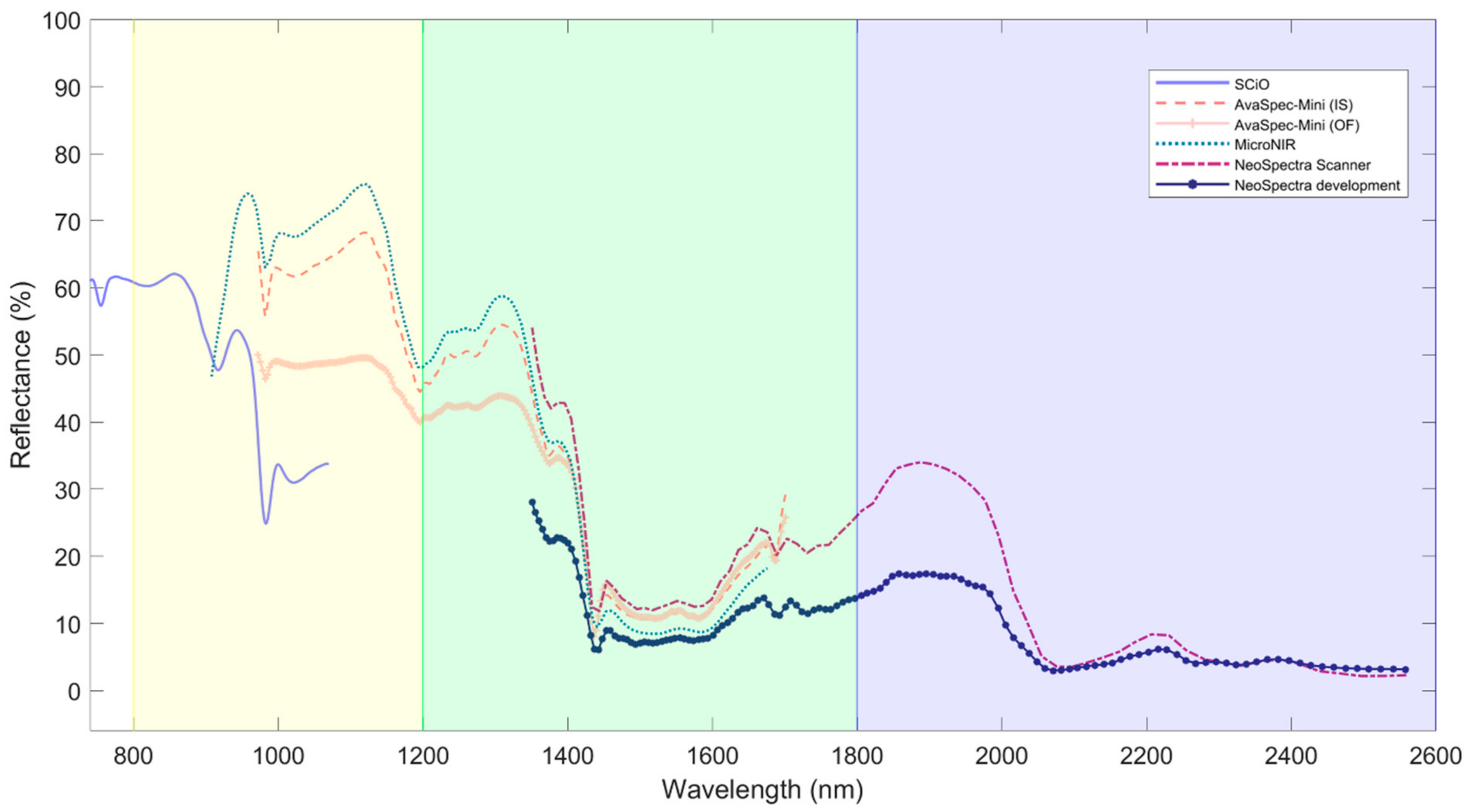
3.1. Spectra and Features
Figure 1 shows the average spectra of granulated sugar collected with the five spectrometers and the two configurations for the AvaSpec-Mini. The different wavelength ranges are also represented. While benchtop instruments typically cover the entire range represented (800–2500 nm) [
33,
34,
35], miniaturized spectrometers typically cover narrower ranges. When dealing with miniaturized sensors, the specific range of acquisition may influence analysis in different ways and careful evaluations need to be pursued for the application of interest. In addition to this, the technological development of different manufacturers should be intended for different scopes, for instance, use in the field or online implementation. With respect to the color [
36,
37] SCiO works in a spectral range that reaches the visible part of the electromagnetic spectrum, adding information that may not be of interest.
A priori knowledge about the applicability of a certain sensor is not straightforward to be evaluated only based on the spectral ranges [
38]. Indeed, when dealing with reflectance NIR spectroscopy the information correlated to the properties of interest is not always strictly related to evident chemical spectral information of the analyte or bulk. On the contrary, it is quite probable that the information is distributed over wider spectral ranges or reflected in the physical information that non-exclusively depends on the spectral range [
7,
39]. Physical parameters, such as compactness and particle sizes, also influence the acquisition of external reflectance NIR spectra because the resulting spectra are strictly related to light path, energy, and power.
The miniaturization and the different engineering designs clearly influenced the working and performance characteristics (e.g., spectral region, sensitivity and precision, spectral resolution, and recordable intensity). Spectra might also be affected by the practical procedures, i.e., sample located near the light source or at a given distance.
Figure 1 shows that even in the regions shared by different devices the signal shapes are slightly different, and the definition of the bands can vary. The overall intensity captured by the spectrometers is also quite different. For the two configurations of Ava-Spec-Mini-NIR it was found that there was, as expected, a higher intensity for the use of the integrating sphere than for the optical fiber. As for the direct comparison of NeoSpectra devices, lower values of reflectance (up to 17%) were registered with the NeoSpectra development kit compared to the Neospectra Scanner. These results could be ascribed to the differences in the spot and detector sizes, the number of light sources (seven tungsten halogen lamps for the Neospectra Scanner and three for the Neospectra development kit), and the analytical measurement procedures.
In
Supplementary Figure S7, the average spectrum of each sample is represented for each analytical configuration and spectrometer. As expected, the red rice reflects the radiation less than the milled rice with every instrument and configuration. The noticeable differences are related to both the physical and chemical differences of the two samples. The comparison of the spectra of granulated and lump sugar highlights the influence of the compactness and granulometry in the investigated spectrometers. Generally, less intense signals were obtained for the sugar lumps even if the difference decreased at higher wavelengths. Peculiar spectra were obtained with SCiO whose spectra showed a consistent change of shape for the different rice samples. The same appeared to be true when comparing the spectra of granulated sugar and brown sugar samples, where their physical and chemical characteristics were identifiable at first sight.
3.2. Exploratory Analysis
The replicates obtained for each sample were used to build an
X matrix, one for each instrument configuration for a total of six datasets. Raw data were centered and then analyzed using Principal Component Analysis (PCA) to detect the presence of gross outliers, which were not detected. In the case of multiple spectra emerging as possible outliers on Hotelling’s T2 and Q residuals statistics, possible trends related to the factors under investigation were studied to understand if they represent the intrinsic variability contained in the experimentations.
Figure 2 shows the score plot obtained for the whole dataset under investigation, whereas in
Figure 3 the loadings are shown. The way in which the replicates and samples are distributed over PC1 and PC2 for the spectrometers is noteworthy. The arrangement of the sample and their dispersion over each sample centroid is characteristic of each sensor. The study of the distribution of samples and replicates may provide interesting insights. The dispersion of the clouds of points related to each sample can be used as semi-quantitative information related to the precision of the analysis. Similar replicas led to closer points in principal component space, while more significant variability in the replicas is reflected in broader disposition.
For what concerns the spectra acquired with different spectrometers and configuration for the same samples, the variability could be related to the interaction between the compactness and sample granulometry and the intrinsic characteristics of the sensors. The influence of different compactness has been partially addressed in [
40], while consideration on different granulometry due to sample pretreatment can be found in [
41]. These topics emerge here as a possible future research direction.
The separation between the five samples is not always accomplished in the scores plot, and it strictly depends on the ability of each spectrometer in capturing the substantial physical and chemical differences among the samples. Overall, sugar lump and granulated sugar spectra seem to have the highest precision for each sensor since the replicates appear closer in the PCA space than those of the other samples. These could be related to the analytical practices along with the sample characteristics; indeed, the presentation of the sample to the sensor is intuitively more constant for the packed form than for the loose one. Other interesting insights came from the fact that when the same sensor is used but different acquisition configurations are selected (
Figure 2c,d), the scores are found to be grouped in different ways, and PCA models explained different percentages of variance. According to the comparison of the loading plots for the AvaSpec−Mini−NIR data (
Figure 3c,d), the distribution of the samples in the score plot could be ascribed to the same spectral regions independently from the acquisition configuration. Indeed, the shape of loadings looked remarkably similar. The differences encountered in the scores could be related to the different detail of the features registered. Neither the acquisition in the same spectral range nor with similar engineering technologies showed the same distribution of the samples (
Figure 2e,f).
All these results lead to the conclusion that it is not straightforward to build a priori theories about instruments’ performances in a specific application. The shapes found in the loadings suggested that both the physical and chemical characteristics of the samples were responsible for the score grouping or dispersion.
It is well known that one of the main sources of repeatability error in spectroscopy is related to scattering effects [
42]. Since the final user is likely to use one of the most common preprocessing techniques for NIR spectra to remove scattering influences, investigations were carried out on how this affects the dataset under study. As for raw data, using MSC (
Supplementary Figures S8 and S9) or SNV (
Supplementary Figures S10 and S11) resulted in different patterns depending on the preprocessing and the spectrometer used for data acquisition.
In the case of SCiO, the use of MSC (which is dependent on the mean spectra of the dataset and corrects for scattering correlated to the wavelength), highly enhances the variability of the red rice while the scores for the spectra of other samples appeared all in the center of the model. The first two components were not sufficient for the discrimination of sample groups. The preprocessing correction was found to be substantially incompatible with the data under investigation, which varied based on chemical, physical, and also color features, the latter highly influencing the SCiO signal. A solution could reside in the use of different reference spectra during the MSC procedure according to the type of sample. On the contrary, when SNV is applied to the data, red rice and brown sugar emerged as distinctive groups, although very separated from the other samples.
Application of the scattering removal preprocessing techniques to MicroNir, AvaSpec, and NeoSpectra Scanner data resulted in very similar outputs. The application of such preprocessing techniques enhances the variability related to the discrimination between samples according to the macroscopic differences between rice and sugar spectra. The use of MSC or SNV did not differently affect the modelling phase. Spectra acquired with the optical fiber were consistently more variable than the ones obtained with the integrating sphere. The variability related to the chemistry of the samples predominantly emerged as the main variance in data, while white granulated and lump sugar samples turned out to be superimposed in the space of the first two PCs.
NeoSpectra development kit spectra showed an interesting behavior for MSC preprocessed data. The main variance (first PC) includes the intrinsic variability of the rice groups while the second component highlights spectroscopic differences between rice and sugar samples. The opposite behavior was found when applying SNV: the first PC was mainly related to the differences between rice and sugar spectra, whereas the second was necessary to explain the variability of the rice sample spectra.
The results obtained after applying spectra preprocessing methods depend on the spectrometer and the samples under investigation, which showed that generalized guidance could not be the most suitable. Consequently, a careful evaluation is needed for the choice of the instrument and the evaluation of the performances for a specific application, even in the case of preprocessing methods.
3.3. Studying the Factors Influencing the Analysis
3.3.1. Preliminary Models
Initially, ASCA models including all the spectra and the spectra divided according to the macro−chemical differences (rice or sugar samples) were calculated and investigated. The multivariate method permitted the separation of the influences of the investigated factors and their interactions. The interpretation of the results is somehow immediate. Some factors resulted significant in different models, whereas others were not, thus allowing the identification of their connection with a specific spectrometer and/or the sample characteristics. The type of sample is the main significant factor in each model that included this source of variability even if with different magnitudes depending on the model and instrument or acquisition configuration considered. Other factors showed a behavior more related to the specific instrument. Results are reported in
Supplementary Tables S1–S5.
3.3.2. ASCA Models on Different Samples
The outcomes of the ASCA models for each sample type were easily evaluated by visualizing and interpreting scores and loadings as in a common PCA. Some selected results for the sub−models obtained are represented in
Figure 4, where some factors significant for the sensors are shown. The obtained scores for the sub−models are represented according to the factor levels, and spider graphs are used to enhance the scores centroid. Tendencies and grouping behaviors reflected the significance of the factors. The results are discussed below according to the spectrometer.
SCiO
ASCA models were carried out on each sample type to enhance the recurrence of significant factors. The influence of spectra preprocessing for scattering removal was also investigated. The results are summarized in
Table 2, which shows the percentage each effect contributes to the sum of squares. The significant effects are highlighted in bold.
From the models of raw spectra, the timing of background emerged as significant for the majority of the samples, whereas other factors and interactions are sparse. For instance, the order of replicates was found significant only for sugar lump spectra, for which the interaction between the order of replicates and the power supply was also significant. When preprocessing was applied to data, interesting results arose. First, the magnitudes of the effects were identical, clearly highlighting that the multiplicative scattering is not present in the data. Secondly, some factors significant for specific samples became negligible when the scattering was removed, whereas others emerged. In general, it is relevant to notice that preprocessing increased the number and extent of significant factors and interactions. A reason could be that when removing the artifacts created by the scattering, the sources of variance typical for the instrument gain importance relative to the variation of the analysis. The sub−model obtained for the factor timing of background of red rice spectra is reported in
Figure 4a,b.
The experimental procedure included the acquisition of brown sugar spectra at the beginning and at the end of each session in order to verify the factor and interaction related to the sample position in the order of analyses. The factor begin or end of the session was considered as well as the interactions with the other factors. No significant effects were found.
MicroNir OnSite−W
The results of ASCA models on each sample group with and without signal preprocessing are summarized in
Table 3, which shows the percentage each effect contributes to the sum of squares. The significative effects are highlighted in bold.
For the raw data, the factor
timing of background, and the interaction between
session × timing of background were significant for all the samples under investigation. The importance of the session of analysis is manifested for almost all the samples. The order of replicates was significant for milled rice and brown sugar (
Figure 4c,d). In addition, the values for the residuals were found to be mainly different depending on the sample considered. This could be ascribed to the concurrence of other factors not taken under control and interactions of higher levels.
Preprocessing was applied to the data and, as for SCiO, the calculated effects were identical showing that the multiplicative scattering is not present in the data. Preprocessing in this case did not change the significant factors and interactions apart from two specific samples with similar particle sizes: session for red rice and session × timing of background for milled rice. Generally, with the higher quality of the preprocessed data, the value of the considered effects increased. An exception was found for the influence of the timing of background, which increased for rice samples and decreased for sugars.
The study conducted to identify if the acquisition of a sample at the beginning or at the end of the session may affect the resulting spectra showed that the factor begin and end of the session had a p−value of 0.075, whereas its interaction with the timing of background had an effect of 15.04 and a p−value of 0.005.
AvaSpec−Mini−NIR
Results for the AvaSpec−Mini−NIR data are summarized for raw and preprocessed data in
Table 4. The significant effects are highlighted in bold.
At a first glance, the significant factors and interactions are the same regardless of acquisition configuration and preprocessing method. The slight differences in the significant effects for the acquisition configuration in raw data could be attributed to the higher intrinsic variability of data acquired with the fiber optic cable compared to the integrating sphere. Indeed, the spectrometer and detector were the same, but the light source and light path through the fiber or the sphere were substantially different, together with the portion of the sample exposed to the acquisition windows. As a general rule, the effect values obtained after the application of MSC or SNV were higher than for raw data and very similar but not identical within them. Interestingly, factors significant only for some samples when raw spectra were considered were found significant for all the samples under investigation when a scattering correction method was applied.
Drawing attention to the factor related to different sessions of analysis and the interaction with the timing of background, interesting aspects arise depending on the samples and configuration. The fact that milled rice spectra resulted in peculiar behavior (only few factors influence the analysis) with integrating sphere configuration could reside in the intrinsic characteristics of the samples, which typically influence NIR acquisition: the grain size and the color.
The factor dealing with the acquisition of brown sugar spectra at the beginning or the end of a session and its interactions with the other factors were investigated. Results allowed for identification of a significant influence of the interaction session × begin or end of the session (effect 3.33 and p−value 0.02) in the spectra obtained with the optical fiber. Data registered with the integrating sphere did not show any significant effect according to the p−values related to the order of samples’ acquisition.
NeoSpectra Scanner
Remarkable aspects were highlighted from the modelling of every single type of sample and the application of signal preprocessing (
Table 5).
Based on the analysis of raw data, session (
Figure 4e,f), timing of background, and power supply are significant factors, as well as their interaction and the interaction with the timing of background. The discrepancy among residual values calculated in these models is consistent depending on the sample, indicating that other factors or higher−level interactions could be involved. The influencing factors in the spectra of this instrument were found substantially independent of scattering removal. The main difference when applying MSC (or SNV) resided in the magnitude of the effects for the significant factors and interactions.
The analysis carried out with the brown sugar spectra acquired at the beginning and the end of the session proved that there is not such a significant influence of the factor itself. In contrast, the interactions session × timing of background, session × begin or end of the session, and timing of background × begin or end of the session were significant (p−values—0.005, 0.025, and 0.005, respectively) with a small contribution (% sum of squares—8.80, 1.77, and 2.01, respectively).
NeoSpectra Development Kit
Looking into the results obtained for each sample (
Table 6), it appears that disparate factors and interactions for different samples could influence the spectra.
None of the factors under investigation were identified as significant from the permutations test for the spectra of rice samples. Despite that, the residuals are compatible with the ones of the previous instruments and with the other samples. The timing of background was found significant with a relatively different magnitude for the spectra of the sugar samples. The same is true for the interaction session × timing of background. Conversely to what was obtained for the other spectrometers, the application of a preprocessing method in this case generally reduced the effect of significant factors, strictly depending on the sample. The order of the sample in the session, investigated through the replicates of brown sugar, demonstrated that the interaction session × begin or end of the session was the only one significant for the spectra acquired by the NeoSpectra development kit.
These results enhanced the importance of a comprehensive study of the signals. In this case, the results of the ASCA models suggested that this spectrometer could be the best option among the tested ones. However, from a thoughtful evaluation of the characteristics of the signal, the circumstances appeared different. First of all, the intensities of the spectra registered with the NeoSpectra development kit were considerably lower than the ones of the spectra acquired with other sensors (
Supplementary Figure S7). The inspection of the S/N ratio and the relative standard deviation was carried out, and results were directly compared with those achieved for the NeoSpectra Scanner spectra. The reason for such comparison resides in the similarity of the sensors’ conceptualization. The S/N was calculated as the ratio between the mean spectra for each sample and the standard deviation of the spectra of the same sample. The relative standard deviation was estimated as 100 × standard deviation of spectra for each sample divided by the mean spectrum for the same sample. In general, the S/N was smaller with the relative standard deviation higher for the Neospectra development kit (
Figure 5). Therefore, fewer factors and interactions were found to be significant in the ASCA models due to the low quality and lack of sensitivity of the sensor and not because of reduced influences in the spectra.
3.4. Emerging Rules of Thumb
The feasibility and utility of miniaturized NIR devices has been proved in the literature in several applications [
2], and the low cost of the sensors mainly led to their wide use in industries of several fields. In addition, the potentialities in gaining chemical and physical information have been widely proved. Despite this, it is quite common to underestimate the importance of the method set−up procedure in the analytical method and the effects to consider during the development of the acquisition strategy [
1]. Under these circumstances, the results obtained through this study are meaningful for several reasons. ASCA allowed the separation of the influences of different factors and interactions on the spectra. Moreover, an esteem of the magnitude of the effects was made available and interpretable through the loadings of each sub−model. Typical behaviors about the main effects studied could be stated for each spectrometer. The class of miniaturized spectrometers is proved to be plenty of differences between technologies and applicability. The outcome for spectrometers measuring the same spectral range could not be expected to be consistent without examining the specific application. Indeed, the intrinsic characteristics of each instrument and the features reflected in different experimental procedures make the influences in the spectra arduous to generalize. Even when the same spectrometer is used but with a different acquisition configuration, as in the case of AvaSpec−Mini−NIR, the variabilities in the data may change. In the same way, the factors to consider can vary depending on how a specific technology is assembled in the final spectrometer, as was proved for NeoSpectra sensors.
Some good practices may pop up from the insights obtained in this work. First, when considering a new application of a miniaturized spectrometer, a previous feasibility analysis has to be carried out for several factors. The method proposed could be used to identify the main factors for the specific case study. Within this frame, the optimization of the background timing was proved essential. Indeed, the acquisition of the background before each sample could be the optimal condition, but being time consuming, the identification of an optimal timing for the parameter is fundamental. Nonetheless, the evaluation of power supply conditions could be of interest when the spectrometer allows analysis standing in battery mode. In some cases, systematic error related to the order of acquisition was identified. Consequently, when more than one experimental replicated spectrum is needed, the influence of subsequent acquisitions is to be taken into consideration, as well as the order of samples under analysis. The general guidelines could reside in the random spectra acquisition for samples with similar characteristics.
With a view to developing predictive or classification models where the ordinary user will likely consider preprocessing methods, a deep investigation must be carried out [
43] according to the emphasized influences found on the factors under study. The calibration set for the modelling phase should be constructed to include the sources of variability related to the instrument and its application [
44,
45] and should consider the reference errors. Similarly, it will most likely be necessary to include the same variabilities for reliable external validation. For instance, if the analysis session is a significant factor, a representative calibration set should include data from different sessions of analyses. Similarly, an actual external validation set could be composed of spectra acquired in different sessions. Other relevant implications could be highlighted for monitoring measurement systems and model maintenance (i.e., the calibration transfer strategies between different instruments and within the same instrument) [
46,
47,
48,
49].


 ,
, 


