
Temperature Modulation of MOS Sensors for Enhanced Detection of Volatile Organic Compounds

 ,
,  , , and
Abstract
:1. Introduction
2. Material and Methods
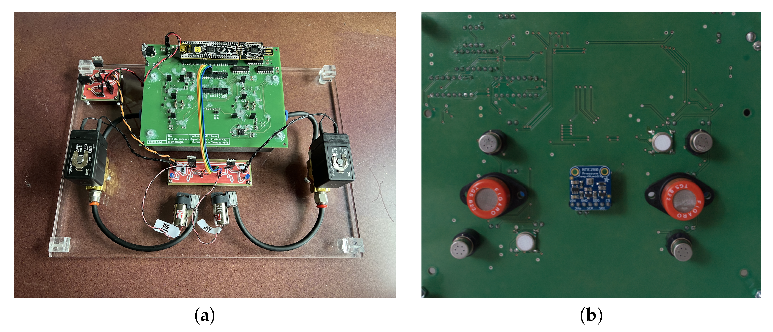
2.1. Hardware
2.1.1. Gas Sensors
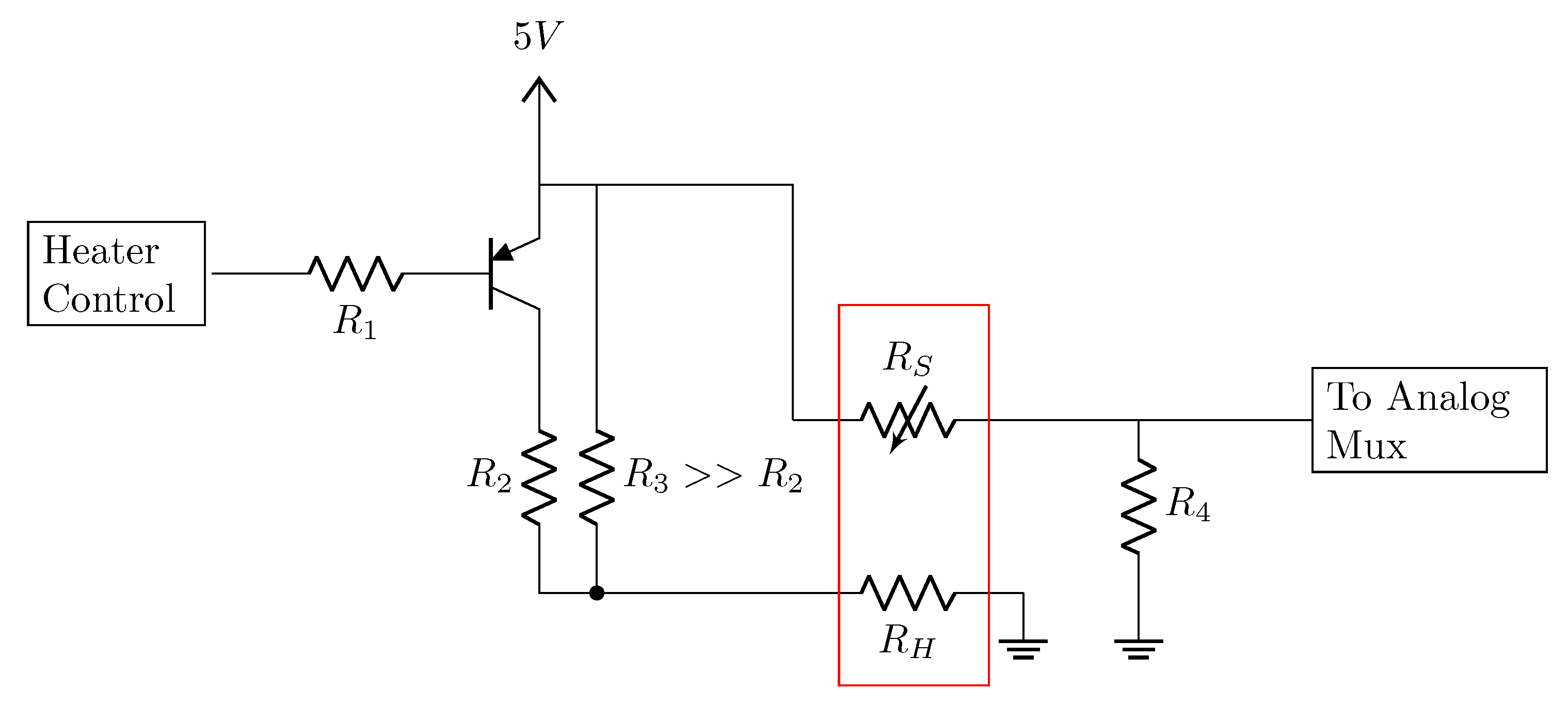
2.1.2. Electronics
2.1.3. Hydraulic Components
2.2. Software
2.3. Experimental Design
- Wash-out (30 min): the first time a new concentration was about to be tested, the chamber and the sensors were cleaned with a continuous stream of pure nitrogen. During this phase, the gas sensors were heated by applying a constant voltage of 5 V.
- Filling (12 min): each time a wash-out phase was performed, it was followed by a 12-min period in which the target analyte was added to the nitrogen flow and introduced inside the chamber. During this phase, the sensor heaters were kept at 5 V. This step was needed to ensure a uniform concentration of the target inside the chamber before measurements.
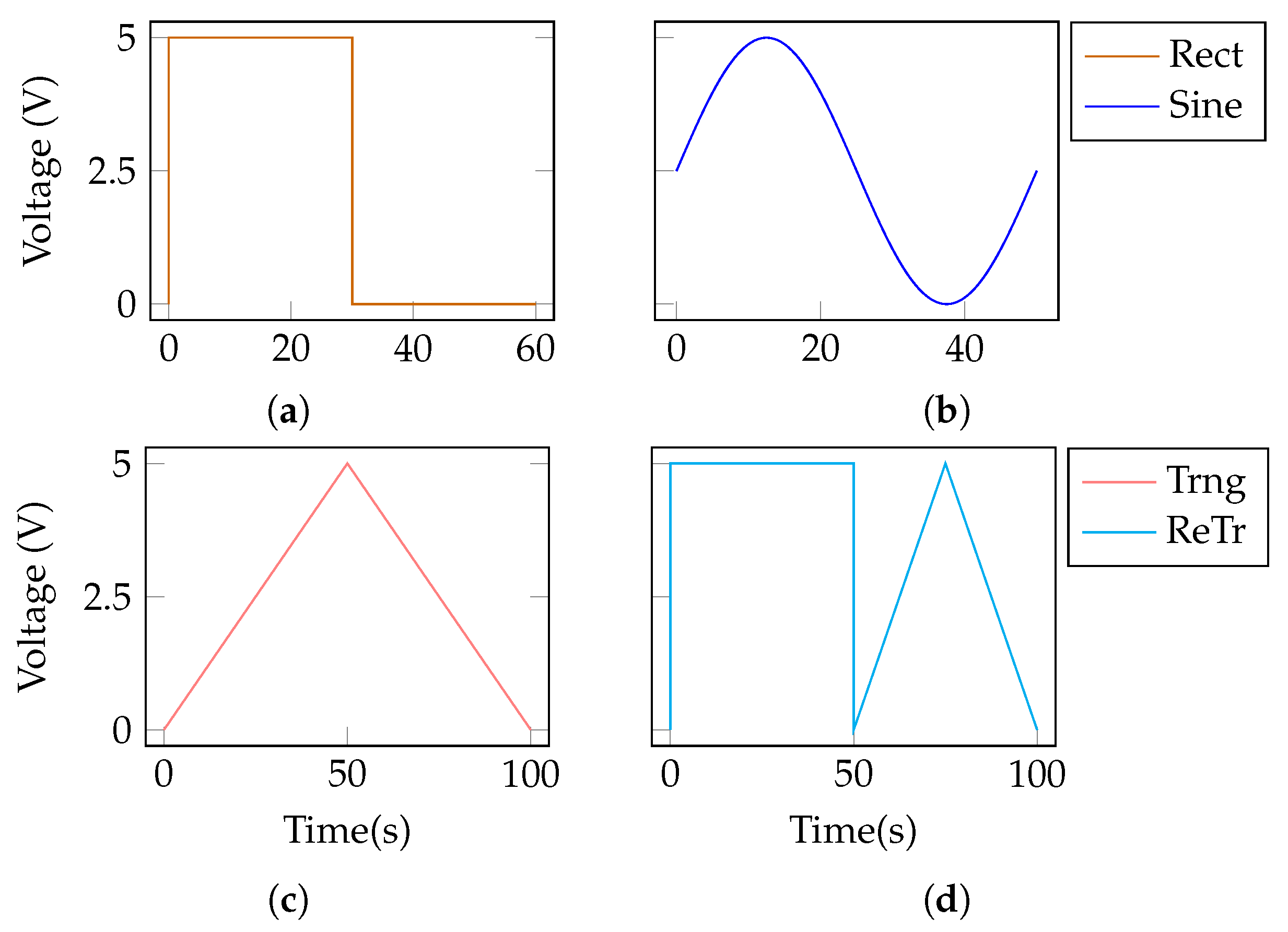
- Modulation (70 min approx.): this phase was divided into three parts:
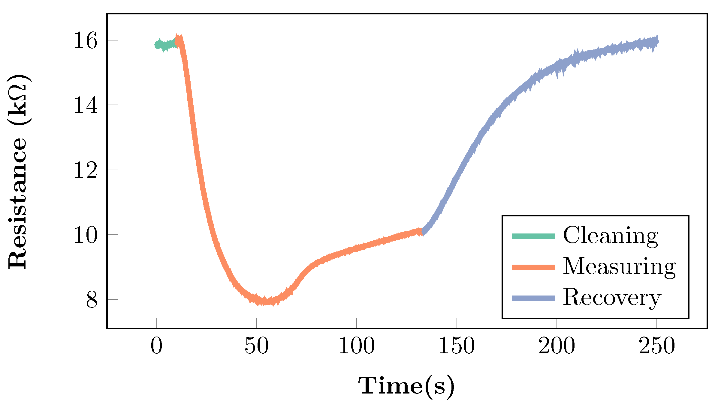
- Baseline: initially, a baseline value for the sensors was measured for 2 min without any pattern applied to the heater.
- Measuring: then, one of the TM patterns was applied for an amount of time sufficient to acquire 10 cycles.
- Recovery: finally, the pattern was interrupted and the heaters were brought back to a constant 5 V for an additional 2 min.
2.4. Data Analysis
2.4.1. Feature Extraction
- : difference between the maximum resistance value of the sensor during the first half of the TM pattern, , and the baseline resistance value of the sensor at time , :
- : difference between the maximum resistance value of the sensor during the first half of the TM pattern, , and the minimum resistance of the sensor during the second half of the TM pattern, . In the case of the ReTr TM pattern, this feature was computed considering the maximum voltage value during the second half of the TM pattern as :
- Slope1: ratio between the value and the time, , required by the sensor to reach the maximum value. This feature allows describing the dynamics of the sensor and the exposure to the sample:
- Slope2: ratio between the value and the time, , required by the sensor to move from the maximum to the minimum value:
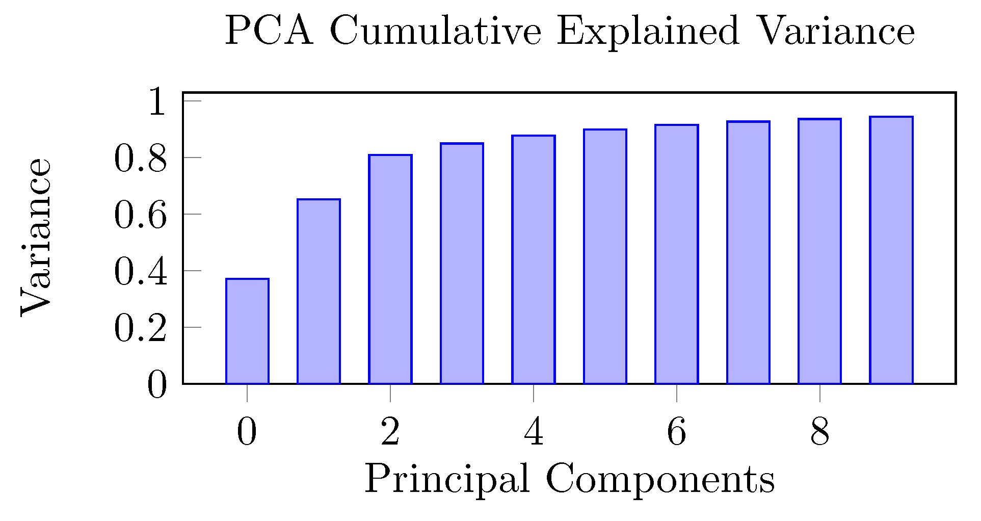
2.4.2. Compound, Concentration, and Sensor Discrimination
3. Experimental Results
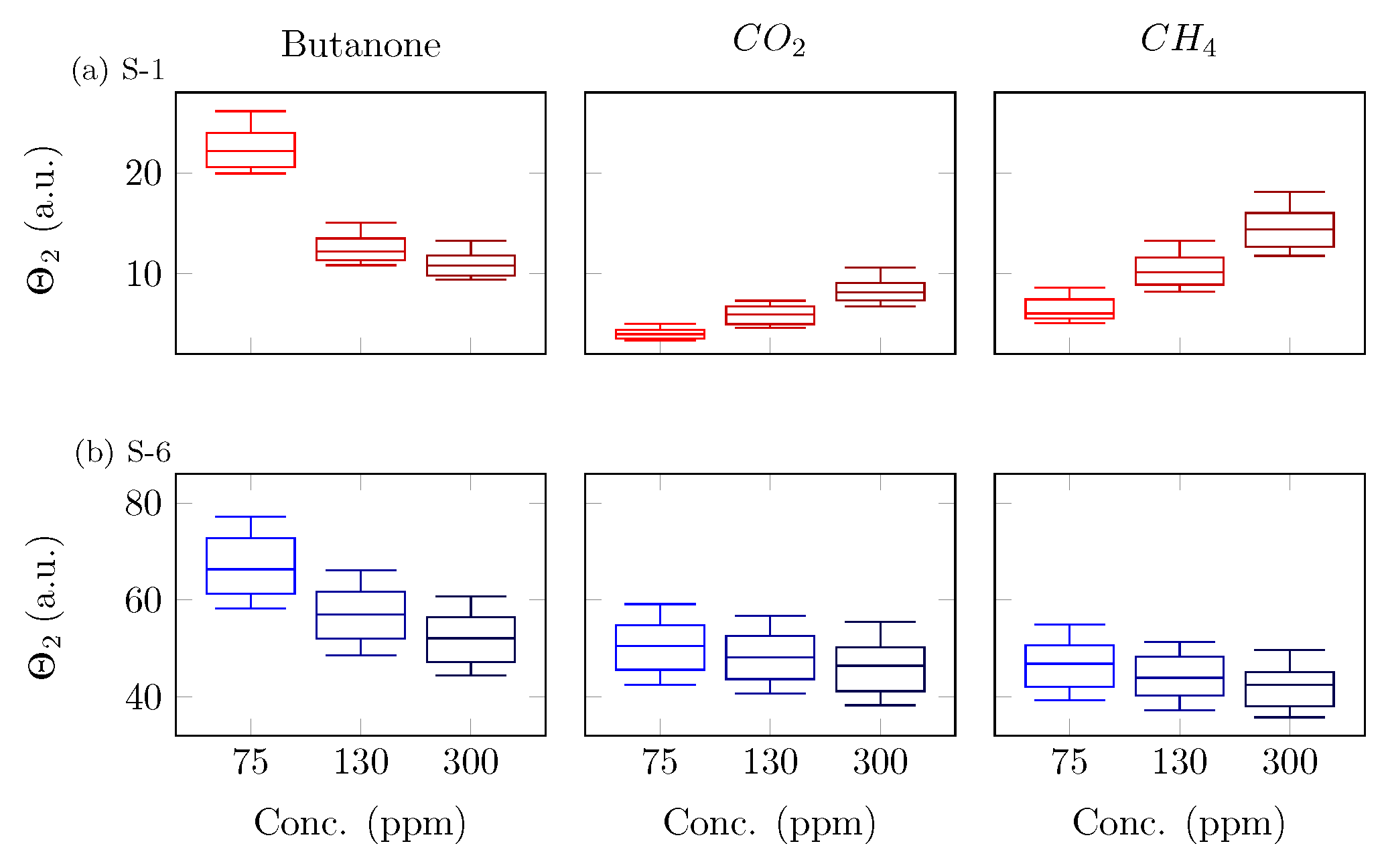
3.1. Features Analysis
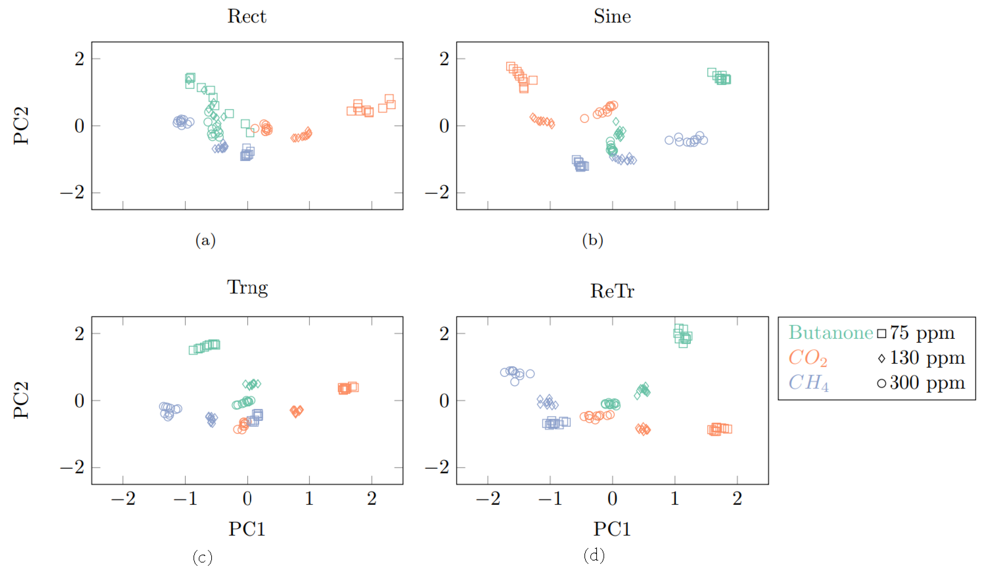
3.2. Temperature Modulation Pattern Dependency
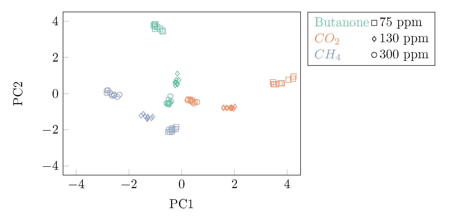
3.3. Sensor Type Dependency
4. Discussion and Conclusions
Author Contributions
Funding
Institutional Review Board Statement
Informed Consent Statement
Data Availability Statement
Acknowledgments
Conflicts of Interest
Abbreviations
| CV | Cross-validation |
| COPD | Chronic obstructive pulmonary disease |
| GC–MS | Gas chromatography–mass spectrometry |
| MOS | Metal oxide semiconductor |
| kNN | k-nearest neighbors |
| LDCT | Low-dose computed tomography |
| PCA | Principal component analysis |
| PCB | Printed circuit board |
| ppb | Parts per billion |
| ppm | Parts per million |
| SVM | Support vector machine |
| VOCs | Volatile organic compounds |
| MCU | Microcontroller unit |
| PTFE | Polytetrafluoroethylene |
| TM | Temperature modulation |
| VOC | Volatile organic compound |
References
- Amann, A.; Miekisch, W.; Schubert, J.; Buszewski, B.; Ligor, T.; Jezierski, T.; Pleil, J.; Risby, T. Analysis of exhaled breath for disease detection. Annu. Rev. Anal. Chem. 2014, 7, 455–482. [Google Scholar] [CrossRef] [PubMed]
- Marzorati, D.; Mainardi, L.; Sedda, G.; Gasparri, R.; Spaggiari, L.; Cerveri, P. A Review of Exhaled Breath: A Key Role in Lung Cancer Diagnosis. J. Breath Res. 2019, 13, 034001. [Google Scholar] [CrossRef] [PubMed]
- Davis, M.D.; Fowler, S.J.; Montpetit, A.J. Exhaled breath testing—A tool for the clinician and researcher. Paediatr. Respir. Rev. 2019, 29, 37–41. [Google Scholar] [CrossRef] [PubMed]
- Dragonieri, S.; Schot, R.; Mertens, B.J.A.; Le Cessie, S.; Gauw, S.A.; Spanevello, A.; Resta, O.; Willard, N.P.; Vink, T.J.; Rabe, K.F.; et al. An electronic nose in the discrimination of patients with asthma and controls. J. Allergy Clin. Immunol. 2007, 120, 856–862. [Google Scholar] [CrossRef] [PubMed]
- Dragonieri, S.; Annema, J.T.; Schot, R.S.; van der Schee, M.P.C.; Spanevello, A.; Carratú, P.; Resta, O.; Rabe, K.F.; Sterk, P.J. An electronic nose in the discrimination of patients with non-small cell lung cancer and COPD. Lung Cancer 2009, 64, 166–170. [Google Scholar] [CrossRef]
- Peng, G.; Hakim, M.; Broza, Y.Y.; Billan, S.; Abdah-Bortnyak, R.; Kuten, A.; Tisch, U.; Haick, H. Detection of lung, breast, colorectal, and prostate cancers from exhaled breath using a single array of nanosensors. Br. J. Cancer 2010, 103, 542–551. [Google Scholar] [CrossRef]
- Hanna, G.B.; Boshier, P.R.; Markar, S.R.; Romano, A. Accuracy and Methodologic Challenges of Volatile Organic Compound–Based Exhaled Breath Tests for Cancer Diagnosis. JAMA Oncol. 2019, 5, e182815. [Google Scholar] [CrossRef]
- Ratiu, I.A.; Ligor, T.; Bocos-Bintintan, V.; Mayhew, C.A.; Buszewski, B. Volatile Organic Compounds in Exhaled Breath as Fingerprints of Lung Cancer, Asthma and COPD. J. Clin. Med. 2021, 10, 32. [Google Scholar] [CrossRef]
- Taverna, G.; Grizzi, F.; Tidu, L.; Bax, C.; Zanoni, M.; Vota, P.; Lotesoriere, B.J.; Prudenza, S.; Magagnin, L.; Langfelder, G.; et al. Accuracy of a new electronic nose for prostate cancer diagnosis in urine samples. Int. J. Urol. 2022, 29, 890–896. [Google Scholar] [CrossRef]
- Montuschi, P. Analysis of exhaled breath condensate in respiratory medicine: Methodological aspects and potential clinical applications. Ther. Adv. Respir. Dis. 2007, 1, 5–23. [Google Scholar] [CrossRef]
- Hakim, M.; Broza, Y.Y.; Barash, O.; Peled, N.; Phillips, M.; Amann, A.; Haick, H. Volatile Organic Compounds of Lung Cancer and Possible Biochemical Pathways. Chem. Rev. 2012, 112, 5949–5966. [Google Scholar] [CrossRef]
- Beccaria, M.; Mellors, T.R.; Petion, J.S.; Rees, C.A.; Nasir, M.; Systrom, H.K.; Sairistil, J.W.; Jean-Juste, M.A.; Rivera, V.; Lavoile, K.; et al. Preliminary investigation of human exhaled breath for tuberculosis diagnosis by multidimensional gas chromatography—Time of flight mass spectrometry and machine learning. J. Chromatogr. B Anal. Technol. Biomed. Life Sci. 2018, 1074–1075, 46–50. [Google Scholar] [CrossRef] [PubMed]
- Marzorati, D.; Mainardi, L.; Sedda, G.; Gasparri, R.; Spaggiari, L.; Cerveri, P. MOS Sensors Array for the Discrimination of Lung Cancer and At-Risk Subjects with Exhaled Breath Analysis. Chemosensors 2021, 9, 209. [Google Scholar] [CrossRef]
- Amor, R.E.; Nakhleh, M.K.; Barash, O.; Haick, H. Breath analysis of cancer in the present and the future. Eur. Respir. Rev. 2019, 28, 190002. [Google Scholar] [CrossRef] [PubMed]
- Rudnicka, J.; Kowalkowski, T.; Ligor, T.; Buszewski, B. Determination of volatile organic compounds as biomarkers of lung cancer by SPME-GC-TOF/MS and chemometrics. J. Chromatogr. B Anal. Technol. Biomed. Life Sci. 2011, 879, 3360–3366. [Google Scholar] [CrossRef]
- Buszewski, B.; Ligor, T.; Jezierski, T.; Wenda-Piesik, A.; Walczak, M.; Rudnicka, J. Identification of volatile lung cancer markers by gas chromatography-mass spectrometry: Comparison with discrimination by canines. Anal. Bioanal. Chem. 2012, 404, 141–146. [Google Scholar] [CrossRef]
- Phillips, M.; Cataneo, R.N.; Cummin, A.R.C.; Gagliardi, A.J.; Gleeson, K.; Greenberg, J.; Maxfield, R.A.; Rom, W.N. Detection of Lung Cancer With Volatile Markers in the Breath. Chest 2003, 123, 2115–2123. [Google Scholar] [CrossRef]
- Machado, R.F.; Laskowski, D.; Deffenderfer, O.; Burch, T.; Zheng, S.; Mazzone, P.J.; Mekhail, T.; Jennings, C.; Stoller, J.K.; Pyle, J.; et al. Detection of Lung Cancer by Sensor Array Analyses of Exhaled Breath. Am. J. Respir. Crit. Care Med. 2005, 171, 1286–1291. [Google Scholar] [CrossRef]
- Bajtarevic, A.; Ager, C.; Pienz, M.; Klieber, M.; Schwarz, K.; Ligor, M.; Ligor, T.; Filipiak, W.; Denz, H.; Fiegl, M.; et al. Noninvasive detection of lung cancer by analysis of exhaled breath. BMC Cancer 2009, 9, 348. [Google Scholar] [CrossRef]
- Ligor, T.; Pater, Ł.; Buszewski, B. Application of an artificial neural network model for selection of potential lung cancer biomarkers. J. Breath Res. 2015, 9, 027106. [Google Scholar] [CrossRef]
- Schallschmidt, K.; Becker, R.; Jung, C.; Bremser, W.; Walles, T.; Neudecker, J.; Leschber, G.; Frese, S.; Nehls, I. Comparison of volatile organic compounds from lung cancer patients and healthy controls-challenges and limitations of an observational study. J. Breath Res. 2016, 10, 046007. [Google Scholar] [CrossRef] [PubMed]
- Kononov, A.; Korotetsky, B.; Jahatspanian, I.; Gubal, A.; Vasiliev, A.; Arsenjev, A.; Nefedov, A.; Barchuk, A.; Gorbunov, I.; Kozyrev, K.; et al. Online breath analysis using metal oxide semiconductor sensors (electronic nose) for diagnosis of lung cancer. J. Breath Res. 2019, 14, 016004. [Google Scholar] [CrossRef] [PubMed]
- Liu, L.; Li, W.; He, Z.; Chen, W.; Liu, H.; Chen, K.; Pi, X. Detection of lung cancer with electronic nose using a novel ensemble learning framework. J. Breath Res. 2021, 15, 026014. [Google Scholar] [CrossRef] [PubMed]
- Dragonieri, S.; Pennazza, G.; Carratu, P.; Resta, O. Electronic Nose Technology in Respiratory Diseases. Lung 2017, 195, 157–165. [Google Scholar] [CrossRef]
- van de Goor, R.; van Hooren, M.; Dingemans, A.M.; Kremer, B.; Kross, K. Training and Validating a Portable Electronic Nose for Lung Cancer Screening. J. Thorac. Oncol. 2018, 13, 676–681. [Google Scholar] [CrossRef]
- Di Natale, C.; Macagnano, A.; Martinelli, E.; Paolesse, R.; D’Arcangelo, G.; Roscioni, C.; Finazzi-Agrò, A.; D’Amico, A. Lung cancer identification by the analysis of breath by means of an array of non-selective gas sensors. Biosens. Bioelectron. 2003, 18, 1209–1218. [Google Scholar] [CrossRef]
- D’Amico, A.; Pennazza, G.; Santonico, M.; Martinelli, E.; Roscioni, C.; Galluccio, G.; Paolesse, R.; Di Natale, C. An investigation on electronic nose diagnosis of lung cancer. Lung Cancer 2010, 68, 170–176. [Google Scholar] [CrossRef]
- Peng, G.; Tisch, U.; Adams, O.; Hakim, M.; Shehada, N.; Broza, Y.Y.; Billan, S.; Abdah-Bortnyak, R.; Kuten, A.; Haick, H. Diagnosing lung cancer in exhaled breath using gold nanoparticles. Nat. Nanotechnol. 2009, 4, 669–673. [Google Scholar] [CrossRef]
- Mazzone, P.J.; Wang, X.F.; Xu, Y.; Mekhail, T.; Beukemann, M.C.; Na, J.; Kemling, J.W.; Suslick, K.S.; Sasidhar, M. Exhaled Breath Analysis with a Colorimetric Sensor Array for the Identification and Characterization of Lung Cancer. J. Thorac. Oncol. 2012, 7, 137–142. [Google Scholar] [CrossRef]
- Zhong, X.; Li, D.; Du, W.; Yan, M.; Wang, Y.; Huo, D.; Hou, C. Rapid recognition of volatile organic compounds with colorimetric sensor arrays for lung cancer screening. Anal. Bioanal. Chem. 2018, 410, 3671–3681. [Google Scholar] [CrossRef]
- Saruhan, B.; Fomekong, R.L.; Nahirniak, S. Review: Influences of Semiconductor Metal Oxide Properties on Gas Sensing Characteristics. Front. Sens. 2021, 2, 657931. [Google Scholar] [CrossRef]
- Wilson, A.D.; Baietto, M. Applications and advances in electronic-nose technologies. Sensors 2009, 9, 5099–5148. [Google Scholar] [CrossRef] [PubMed]
- Blatt, R.; Bonarini, A.; Calabro, E.; Torre, M.D.; Matteucci, M.; Pastorino, U. Lung Cancer Identification by an Electronic Nose based on an Array of MOS Sensors. In Proceedings of the 2007 International Joint Conference on Neural Networks, Orlando, FL, USA, 12–17 August 2007. [Google Scholar] [CrossRef]
- Kou, L.; Zhang, D.; Liu, D. A Novel Medical E-Nose Signal Analysis System. Sensors 2017, 17, 402. [Google Scholar] [CrossRef] [PubMed]
- Santos, V.; Freitas, C.; Fernandes, M.G.; Sousa, C.; Reboredo, C.; Cruz-Martins, N.; Mosquera, J.; Hespanhol, V.; Campelo, R. Liquid biopsy: The value of different bodily fluids. Biomark. Med. 2022, 16, 127–145. [Google Scholar] [CrossRef] [PubMed]
- Ulanowska, A.; Kowalkowski, T.; Trawińska, E.; Buszewski, B. The application of statistical methods using VOCs to identify patients with lung cancer. J. Breath Res. 2011, 5, 046008. [Google Scholar] [CrossRef]
- Rudnicka, J.; Kowalkowski, T.; Buszewski, B. Searching for selected VOCs in human breath samples as potential markers of lung cancer. Lung Cancer 2019, 135, 123–129. [Google Scholar] [CrossRef]
- Sears, W.; Colbow, K.; Consadori, F. Algorithms to improve the selectivity of thermally-cycled tin oxide gas sensors. Sens. Actuators 1989, 19, 333–349. [Google Scholar] [CrossRef]
- Cavicchi, R.; Suehle, J.; Kreider, K.; Gaitan, M.; Chaparala, P. Fast temperature programmed sensing for micro-hotplate gas sensors. IEEE Electron. Device Lett. 1995, 16, 286–288. [Google Scholar] [CrossRef]
- Cavicchi, R.; Suehle, J.; Kreider, K.; Gaitan, M.; Chaparala, P. Optimized temperature-pulse sequences for the enhancement of chemically specific response patterns from micro-hotplate gas sensors. Sens. Actuators B Chem. 1996, 33, 142–146. [Google Scholar] [CrossRef]
- Hossein-Babaei, F.; Amini, A. A breakthrough in gas diagnosis with a temperature-modulated generic metal oxide gas sensor. Sens. Actuators B Chem. 2012, 166–167, 419–425. [Google Scholar] [CrossRef]
- Martinelli, E.; Polese, D.; Catini, A.; D’Amico, A.; Di Natale, C. Self-adapted temperature modulation in metal-oxide semiconductor gas sensors. Sens. Actuators B Chem. 2012, 161, 534–541. [Google Scholar] [CrossRef]
- Gosangi, R.; Gutierrez-Osuna, R. Active Temperature Programming for Metal-Oxide Chemoresistors. IEEE Sens. J. 2010, 10, 1075–1082. [Google Scholar] [CrossRef]
- Wu, Z.; Zhang, H.; Ji, H.; Yuan, Z.; Meng, F. Novel combined waveform temperature modulation method of NiO-In2O3 based gas sensor for measuring and identifying VOC gases. J. Alloys Compd. 2022, 918, 165510. [Google Scholar] [CrossRef]
- Li, W.; Liu, H.; Xie, D.; He, Z.; Pi, X. Lung Cancer Screening Based on Type-different Sensor Arrays. Sci. Rep. 2017, 7, 1969. [Google Scholar] [CrossRef] [PubMed]
- Infineon Technologies. PSoC 5LP: CY8C58LP Family Datasheet; Cypress Semiconductor Corporation: San Jose, CA, USA, 2019. [Google Scholar]
- Robert Bosch GmbH. BME280 Datasheet; Bosch Sensortec: Kusterdingen, Germany, 2018. [Google Scholar]
- de Lacy Costello, B.P.J.; Ledochowski, M.; Ratcliffe, N.M. The importance of methane breath testing: A review. J. Breath Res. 2013, 7, 024001. [Google Scholar] [CrossRef]
- Szabó, A.; Ruzsanyi, V.; Unterkofler, K.; Mohácsi, A.; Tuboly, E.; Boros, M.; Szabó, G.; Hinterhuber, H.; Amann, A. Exhaled methane concentration profiles during exercise on an ergometer. J. Breath Res. 2015, 9, 016009. [Google Scholar] [CrossRef]
- Fu, X.A.; Li, M.; Knipp, R.J.; Nantz, M.H.; Bousamra, M. Noninvasive detection of lung cancer using exhaled breath. Cancer Med. 2014, 3, 174–181. [Google Scholar] [CrossRef]
- Wang, C.; Yin, L.; Zhang, L.; Xiang, D.; Gao, R. Metal oxide gas sensors: Sensitivity and influencing factors. Sensors 2010, 10, 2088–2106. [Google Scholar] [CrossRef]
- Amini, A.; Bagheri, M.A.; Montazer, G.A. Improving gas identification accuracy of a temperature-modulated gas sensor using an ensemble of classifiers. Sens. Actuators B Chem. 2013, 187, 241–246. [Google Scholar] [CrossRef]
- Yin, X.; Zhang, L.; Tian, F.; Zhang, D. Temperature Modulated Gas Sensing E-Nose System for Low-Cost and Fast Detection. IEEE Sens. J. 2016, 16, 464–474. [Google Scholar] [CrossRef]
- Sriyudthsak, M.; Promsong, L.; Panyakeow, S. Effect of carrier gas on response of oxide semiconductor gas sensor. Sens. Actuators B Chem. 1993, 13, 139–142. [Google Scholar] [CrossRef]
- Shah, A.; Laurent, O.; Lienhardt, L.; Broquet, G.; Rivera Martinez, R.; Allegrini, E.; Ciais, P. Characterising the methane gas and environmental response of the Figaro Taguchi Gas Sensor (TGS) 2611-E00. Atmos. Meas. Tech. 2023, 16, 3391–3419. [Google Scholar] [CrossRef]


| Sensor | Sensitivity [ppm] | Target Compounds |
|---|---|---|
| TGS2600 | 1–100 | methane, ethanol, hydrogen |
| TGS822 | 50–5000 | Organic solvent vapors (methane, benzene, …) |
| AS-MLV-P2 | 10–5000 | Reducing gases (carbon oxide, methane, …) |
| Butanone | CO2 | CH4 | |||||||
|---|---|---|---|---|---|---|---|---|---|
| Sensor | 75 | 130 | 300 | 75 | 130 | 300 | 75 | 130 | 300 |
| S-1 (TGS2600) | 1400 | 1103 | 804.0 | 288.8 | 350.8 | 529.3 | 376.2 | 650.7 | 1021 |
| S-6 (TGS822) | 3388 | 3279 | 3097 | 4721 | 3939 | 3570 | 3042 | 2924 | 2784 |
| S-7 (AS-MLV-P2) | 12,103 | 2645 | 1039 | 6.4 | 2.2 | 1.1 | 31,969 | 1.6 | 2.8 |
Disclaimer/Publisher’s Note: The statements, opinions and data contained in all publications are solely those of the individual author(s) and contributor(s) and not of MDPI and/or the editor(s). MDPI and/or the editor(s) disclaim responsibility for any injury to people or property resulting from any ideas, methods, instructions or products referred to in the content. |
© 2023 by the authors. Licensee MDPI, Basel, Switzerland. This article is an open access article distributed under the terms and conditions of the Creative Commons Attribution (CC BY) license (https://creativecommons.org/licenses/by/4.0/).
Share and Cite
Rescalli, A.; Marzorati, D.; Gelosa, S.; Cellesi, F.; Cerveri, P. Temperature Modulation of MOS Sensors for Enhanced Detection of Volatile Organic Compounds. Chemosensors 2023, 11, 501. https://doi.org/10.3390/chemosensors11090501
Rescalli A, Marzorati D, Gelosa S, Cellesi F, Cerveri P. Temperature Modulation of MOS Sensors for Enhanced Detection of Volatile Organic Compounds. Chemosensors. 2023; 11(9):501. https://doi.org/10.3390/chemosensors11090501
Chicago/Turabian StyleRescalli, Andrea, Davide Marzorati, Simone Gelosa, Francesco Cellesi, and Pietro Cerveri. 2023. "Temperature Modulation of MOS Sensors for Enhanced Detection of Volatile Organic Compounds" Chemosensors 11, no. 9: 501. https://doi.org/10.3390/chemosensors11090501
APA StyleRescalli, A., Marzorati, D., Gelosa, S., Cellesi, F., & Cerveri, P. (2023). Temperature Modulation of MOS Sensors for Enhanced Detection of Volatile Organic Compounds. Chemosensors, 11(9), 501. https://doi.org/10.3390/chemosensors11090501