Article

A New X-ray Diffraction Spectrum-Based Untargeted Strategy for Accurately Identifying Ancient Painted Pottery from Various Dynasties and Locations in China

1
Ningxia Institute of Cultural Relics and Archeology, Yinchuan 750001, China
2
The Guyuan Museum of Ningxia, Guyuan 756000, China
3
College of Pharmacy, Ningxia Medical University, Yinchuan 750004, China
*
Authors to whom correspondence should be addressed.
Chemosensors 2024, 12(4), 64; https://doi.org/10.3390/chemosensors12040064
Submission received: 26 December 2023 / Revised: 3 March 2024 / Accepted: 8 March 2024 / Published: 15 April 2024
(This article belongs to the Special Issue Chemometrics for Analytical Chemistry: Second Edition)

Abstract

:
X-ray diffraction (XRD) is extensively used in archaeometric investigation. Herein, we provide a novel XRD spectrum-based untargeted strategy for the classification of ancient painted pottery for various dynasties. It was accomplished using the original spectrum without a phase identification. To eliminate the influence of baseline drift, a new baseline drift correction algorithm was specifically designed for XRD spectra. The algorithm was implemented using local minimum values in the analyzed signal in an iterative optimization manner. The results indicated that with the aid of the algorithm, the baseline drift problem can be successfully resolved, and the classification of ancient painted pottery can be greatly improved. Finally, the developed strategy was successfully used to discriminate ancient painted pottery from the Han and Tang dynasties in the cities of Guyuan and Zhongwei, China. The developed untargeted strategy had the remarkable advantage of almost automatic data analysis. The toolbox of our strategy can be obtained from the authors.

1. Introduction

Pottery plays an important role in human history. A comprehensive investigation of the development of ancient pottery can help explore the culture, economic development, and routine way of life of ancient people [1,2,3,4,5,6]. Accurately identifying pottery samples during archaeological excavations can provide evidence for scientific research, and a number of sophisticated analytical techniques have been introduced to achieve this goal [7,8,9,10,11,12,13]. X-ray diffraction (XRD) is widely used for the analysis of ancient pottery samples. For instance, Aoyama et al. [14] used non-destructive elemental analysis for pottery samples from the zones of Japan Jomon and Neolithic China. Wu et al. [6] used X-ray fluorescence to study the long-distance trade of white pottery in Neolithic China. Gajić-Kvaš č ev et al. studied painted pottery samples from different periods [4].
Most studies have been performed on the basis of glazed pottery [1,3,6,13,15,16,17,18,19]. With respect to other types like ancient painted pottery, mostly used as funerary objects, few studies have been reported. A trait of this ancient painted pottery is that it was not traded or used in ancient society, so it can serve as a direct reflection of society’s development at that time. Historically, Guyuan and Zhongwei were key points in the Silk Road that connected ancient China with the “West”. The study of painted funerary potteries from the two cities can be greatly helpful for recognizing cultural integration in ancient China [5]. Unfortunately, the lack of firing step in the production of the painted funerary pottery caused the painted materials on the surface to readily fall off during the long burial period.
Pottery needs to be recognized from different locations and dynasties in routine work. X-ray diffraction (XRD) techniques are extensively used for tracing ancient glazed pottery [8,9], but their application in painted funerary pottery remains limited. Conventional analysis of XRD data heavily relies on the experience of analysts. Previous knowledge is needed to deconvolute XRD peaks to extract deduced mineralogical composition and subsequently characterize analyzed potteries. A number of unidentified XRD peaks in the XRD spectra are abandoned during data analysis, even if they may be helpful for tracing painted pottery. On the other hand, the selection of various standard cards can result in quite different results for mineralogical composition, which may puzzle users without additional valid information about the analyzed samples.
Theoretically, the use of an entire XRD spectrum to perform an untargeted data analysis can also provide classification results for ancient painted pottery samples. A remarkable advantage is that the risk of incorrect deconvolution can be greatly reduced. Meanwhile, the data analysis efficiency can be improved. However, few works have been published using the entire XRD spectrum for pottery discrimination. A very possible reason is the baseline drift problem in the analyzed complex samples [20]. The presence of baseline drift can affect the qualitative resolution of an XRD spectrum and introduce bias into the quantitative results, thereby providing inaccurate classification results for painted pottery samples [21,22]. Most studies have been conducted using a manual baseline drift correction strategy, in which experienced analysts select several data points in an analyzed XRD spectrum to estimate baselines with curve-fitting algorithms. Although a number of state-of-the-art baseline drift correction algorithms [22,23] have been developed and used for techniques such as Raman and chromatogram analysis, their performance on XRD analysis has not been demonstrated. In conclusion, an automatic strategy for correcting baseline drifts in an XRD spectrum to provide classification results for ancient pottery samples remains lacking.
In the present study, we developed a novel XRD spectrum-based untargeted strategy for the discrimination of ancient painted funerary pottery, which is accomplished by using the raw XRD spectrum of pottery as the input to automatically perform baseline drift correction and chemometric analysis without a manual selection of underlying mineralogical composition. A remarkable advantage of the developed untargeted strategy was that there is no need for the deconvolution of XRD peaks, and thus, archaeologists can perform data analysis by themselves to focus on the collected pottery. A new baseline drift correction algorithm was specifically designed for the XRD spectrum in our strategy. The developed untargeted strategy was demonstrated by discriminating ancient pottery samples of the Han and Tang dynasties from the cities of Guyuan and Zhongwei in Ningxia Province, China.

2. Experiment and Methodology

2.1. Experiment

2.1.1. Painted Pottery Collection

In ancient China, painted funerary pottery was fabricated by painting various colorful pigments on the pottery surface. A total of 22 painted funerary pottery pieces were collected during a series of archaeological excavations in the cities of Guyuan and Zhongwei in Ningxia, China. The archaeologists classified these potteries into 11 red potteries and 11 white potteries according to the color of major pigments on the surface, and typical examples are shown in Figure S1, Supplementary Materials. All these potteries were found in ancient tombs concluded to belong to the Han and Tang dynasties according to archaeologists.
For the 11 red potteries, 8 potteries were found in the tombs of Zhongwei City, including 6 potteries from the Han dynasty (202–220 BC) and 2 from the Tang dynasty (AD 618–690). The remaining 3 red potteries were found in the Han tombs of Guyuan City. Similarly, among the 11 white potteries, 8 were collected from the Zhongwei City, comprising 6 Han tombs and 2 Tang tombs. The remaining 3 white potteries were excavated from the Han tomb of Guyuan City. Powder samples of each pottery were collected by carefully scraping the pigments on the surface. Specifically, only the red and white pigments were selected for the powder sample collection of red and white potteries, respectively. For each pottery, several positions were randomly selected, and no more than 1 g of powder was collected. The powder samples were directly used for both XRD and energy-dispersive X-ray spectroscopy (EDS) analysis.

2.1.2. XRD Analysis

XRD analysis was performed on an UltimaIV (Rigaku, Tokyo, Japan). Parameters were set as follows: anode in the device, CuKα; wave, 1.5419 nm; voltage, 40 kV; and current, 40 mA. The 2θ scanning range was set as 5°–90° at a step of 0.02°. For each sample, a single spectrum was collected. Mineralogical analysis was performed by experienced analysts using some previous knowledge of some common compositions of artifacts. Semi-quantitative analysis was conducted based on the RIR method, and the results are shown in Tables S1 and S2.

2.1.3. EDS analysis

The powder (about 0.5 g) of each pottery was placed into a circle molding and then Technovit EPOX (Hanau, Germany) resin (9 g) and Technovit EPOX HARDENER (1.286 g) were added. Five rounds of grinding were used after demolding. Finally, the prepared sample was analyzed by EDS. A spectrometer AztecOne XT EDS (Oxford X) with a TEMJEOL 2100F microscope (Oxford, UK) was used for EDS analysis. The parameters were as follows: accelerating voltage, 20 kV; spot size, 7.0 nm; working distance, 10 mm; and quantification algorithm, PB/ZAF. The element of C was eliminated. The contents of detected elements were normalized to 100% and shown in Tables S1 and S2 as well.

2.2. Methodology

The developed XRD spectrum-based untargeted strategy primarily involved baseline drift correction and chemometric analysis. The baseline drift correction for the XRD spectrum was described in detail, which was accomplished based on the local minimal values in analyzed signals [21] and comprised local minimal value detection, outlier detection, and baseline estimation.

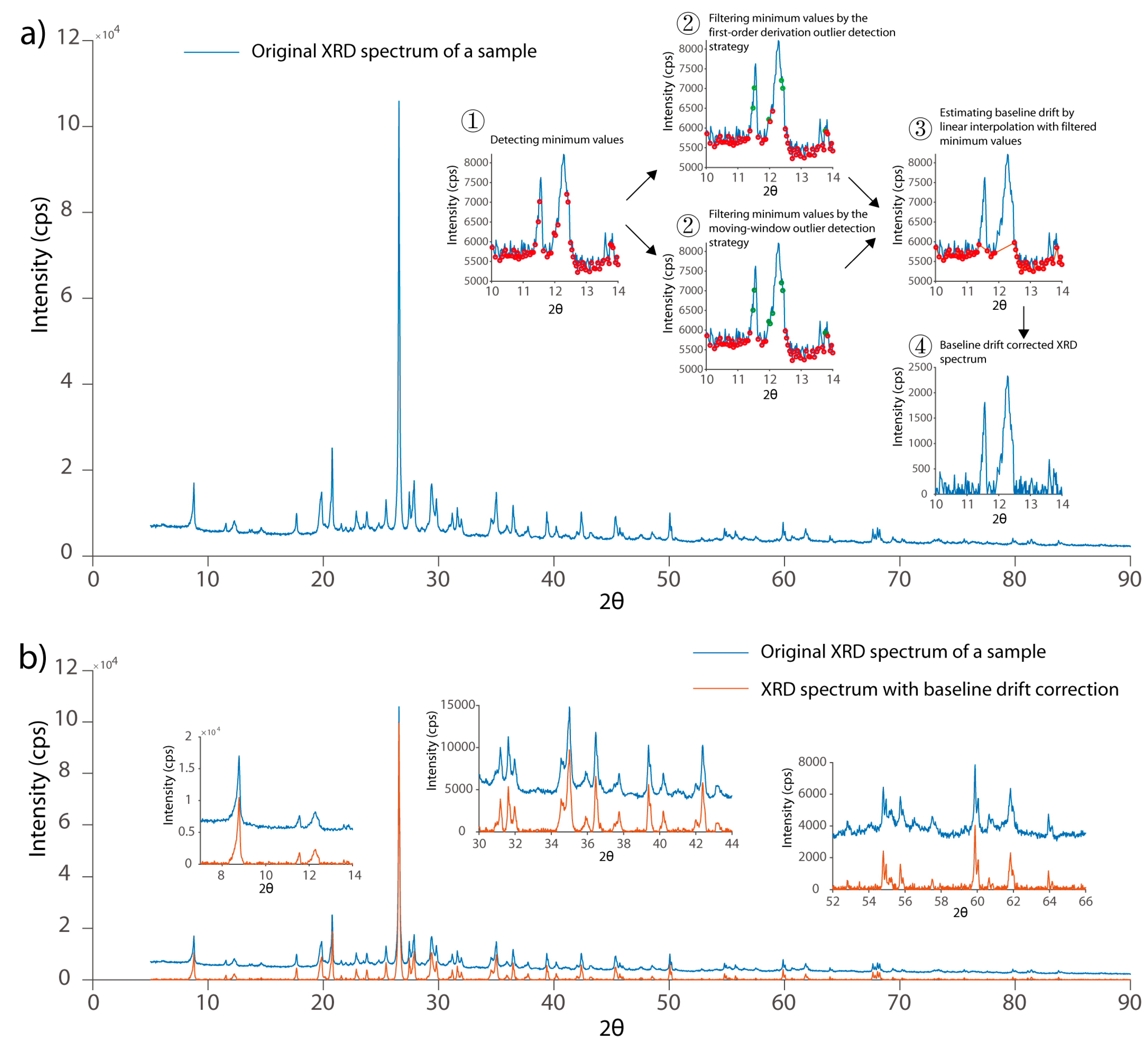
2.2.1. Local Minimum Detection

Mathematically, an XRD spectrum can be divided into three parts, namely, information from chemical compositions, baseline drift, and instrument noise:
s = x + b + e ,
where s, x, and b are vectors corresponding to the recorded XRD spectrum, signals of chemical compositions, and baseline drift in the spectrum, respectively; and e is the instrument noise. The purpose of baseline drift correction was to find an approximate for the vector b. Our strategy first detected minimum values in s by using the following equation:
s i 1 > s i   a n d   s i < s i + 1 ,
where si, si−1, and si+1 represent the ith, i−1th, and i+1th elements in the spectrum, respectively. The extracted local minimum values are illustrated in the inserted plot of Figure 1a (step 1), where all local minimum values in the XRD spectrum are depicted. Apart from the local minimum values belonging to baseline drifts, those from XRD peaks can also be extracted. They must be removed precisely to avoid signal distortion. Here, an outlier detection strategy was designed.

2.2.2. Outlier Detection

To accurately distinguish local minimum values from baseline drift and those from XRD peaks, an outlier detection strategy was designed. The intensities corresponding with the minimum values from the baseline drift usually changed gently across the entire spectrum, whereas the intensities of those from XRD peaks dramatically increased (step 1 in Figure 1a). Thus, the principle behind baseline drift correction was that the correction procedure could be transformed into a problem that accurately detected outliers from the local minimum values. To achieve this goal, the following first-order derivation-based outlier detection equation was used in our strategy:
d i = v i v i 1 ,
where di is the first-order derivation of the ith element; and vi and vi−1 are the ith and i−1th minimum values in the local minimum vector v, respectively. The first-order derivation of v was marked as another vector d, whose standard derivation was determined using a robust statistical manner as follows:
ε = 1.483 * med d m e d ( d ) ,
where ε is the robust standard derivation of d; “med” is the median value of a vector; and 1.483 is a correction factor to make ε obey normal distribution. If an element of v (such as vj) obtained its first-order derivation (e.g., dj) and was three times larger than the robust standard derivation ε, it would be recognized as an outlier and be removed from the vector v. In our strategy, an iteration strategy was used, whose sub-steps can be described as follows:
(i)
The first-order derivation vector d was calculated based on the original local minimum vector vorg;
(ii)
The robust statistical standard derivation ε was estimated according to Equation (4);
(iii)
The outliers whose first-order derivation values exceed 3 * ε were identified and replaced with a linear interpolation strategy to obtain a new vector vnew;
(iv)
vorg was replaced with vnew, and sub-steps (i) to (iii) were repeated until no outliers remained.
According to the above-mentioned four steps, the outliers in the local minimum vector were iteratively removed. Owing to the complexity of the analyzed samples, one may encounter the problem that outliers in the local minimum values cannot always be accurately identified by the first-order derivation strategy, especially for those continuously appearing in the spectrum. To address this problem, we introduced a moving window-based outlier detection strategy in our algorithm as well. The original local minimum vector from Equation (2) vorg was smoothed with a moving window strategy, whose window size was designed by default as 31 data points. For each window, the central point was compared with the smoothed one as follows:
s i = v i med w i / ε ,
where wi is the moving window of the ith data points in vorg. All elements in wi were also extracted from vorg. si can be treated as the signal-to-noise ratio of vi. If the value of si was above 3, vi would be treated as an outlier and removed from the vector vorg. To efficiently remove all outliers in vorg, an iterative optimization algorithm was designed as follows:
(i)
For each element in the original local minimum vector vorg, its signal-to-noise ratio was calculated according to Equation (5).
(ii)
The outliers whose signal-to-noise ratios exceeded 3 were identified and replaced through linear interpolation to obtain a new vector vnew.
(iii)
vorg was replaced with vnew, and sub-steps (i) to (iii) were repeated until convergence. The criterion of convergence was set as v n e w v o r g / v o r g < 10 6 , where .   represents the Frobenius norm.
In our XRD baseline drift correction strategy, if an element in the local minimum vector v was found as an outlier by either the first-order derivation strategy or the moving window smoothing strategy, it would be eliminated from the vector.

2.2.3. Estimation for Baseline Drift

The baseline drift was estimated with the remaining elements in v through simple linear interpolation, as illustrated in the third plot of Figure 1a (step 3). After detecting the local minimum values in the signal (step 1), outliers were recognized from the first-order derivation strategy and the moving window smoothing strategy (step 2), as shown in the inserted plots. The estimated baseline drift was estimated by linear interpolation on the basis of the remaining local minimum values (step 3). Finally, the corrected signal with baseline drift correction was obtained after removing the baseline drift (step 4). An overview of the XRD spectrum with baseline drift correction is shown in Figure 1b. Figure 1b shows that the baseline drift in various parts of the spectrum was properly corrected. The XRD peaks in the spectrum were accurately maintained.

2.3. Chemometric Analysis

A Matlab GUI, AntDAS-XRD, was developed for users to benefit from their data analysis. It was written in the Matlab environment. The GUI of AntDAS-XRD is shown in Figure S2, which can be made available by the authors. Raw XRD spectra were imported into our developed AntDAS-XRD to perform baseline drift correction. Additionally, data pretreatments like mean-centering and autoscaling can also be supported within the GUI. Chemometric methods like principal component analysis (PCA) and partial least square discrimination analysis (PLS-DA) can be performed within the GUI.

3. Results and Discussion

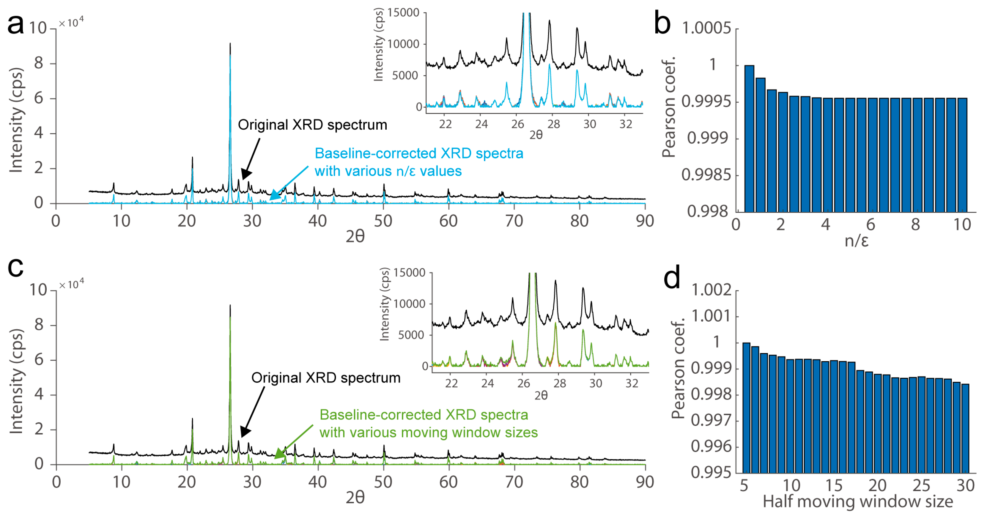
3.1. Investigation of Initialized Parameters on the Quality of Baseline Drift Correction

Our XRD baseline drift correction method required two manually preset parameters to perform baseline drift correction, i.e., the cutoff value for signal-to-noise ratios in Equation (3) and the moving window size in Equation (5). Here, the quality of baseline drift correction was investigated by setting various values for the two parameters, and the results are shown in Figure 2. Specifically, Figure 2a,b provide the baseline drift correction results corresponding with various cutoff values of the first-order derivation. Meanwhile, those corresponding with various moving window sizes are shown in Figure 2c,d. The profiles in Figure 2a evidently indicated a baseline drift in the original XRD spectrum. The developed strategy can provide satisfactory baseline drift correction at various cutoff values because the corrected XRD spectra corresponding with various cutoff values were almost identical to one another. Pearson coefficients were then used to quantitatively evaluate the similarity of the corrected spectra under various cutoff values. One can find that all corrected spectra can obtain high Pearson coefficients above 0.999, indicating that the developed method was insensitive to the initialized cutoff value for signal-to-noise ratios in Equation (3).
The effect of moving window size on baseline drift correction was studied as well. Moving windows with half window size (N) that varied from 5 to 30 data points were investigated, and the results are shown in Figure 2c. The baseline drift problem in the original XRD spectrum can be efficiently corrected by the developed method under various window sizes by providing corrected spectra that are almost identical to one another. Quantitative evaluation was performed using the Pearson coefficients of the corrected spectra. The results indicated that the similarities of corrected spectra were above 0.998 (Figure 2d), implying the developed method was insensitive to the moving window size.
As shown in Figure 2, the developed XRD baseline drift correction strategy was insensitive to the two initialized parameters involving the cutoff value for signal-to-noise ratios in Equation (3) and the moving window size in Equation (5). Accordingly, the XRD data analysis can be almost automatically performed without manual optimization. Herein, the values of 3 and 31 were used for the cutoff value of the signal-to-noise ratio and the moving window size, respectively.

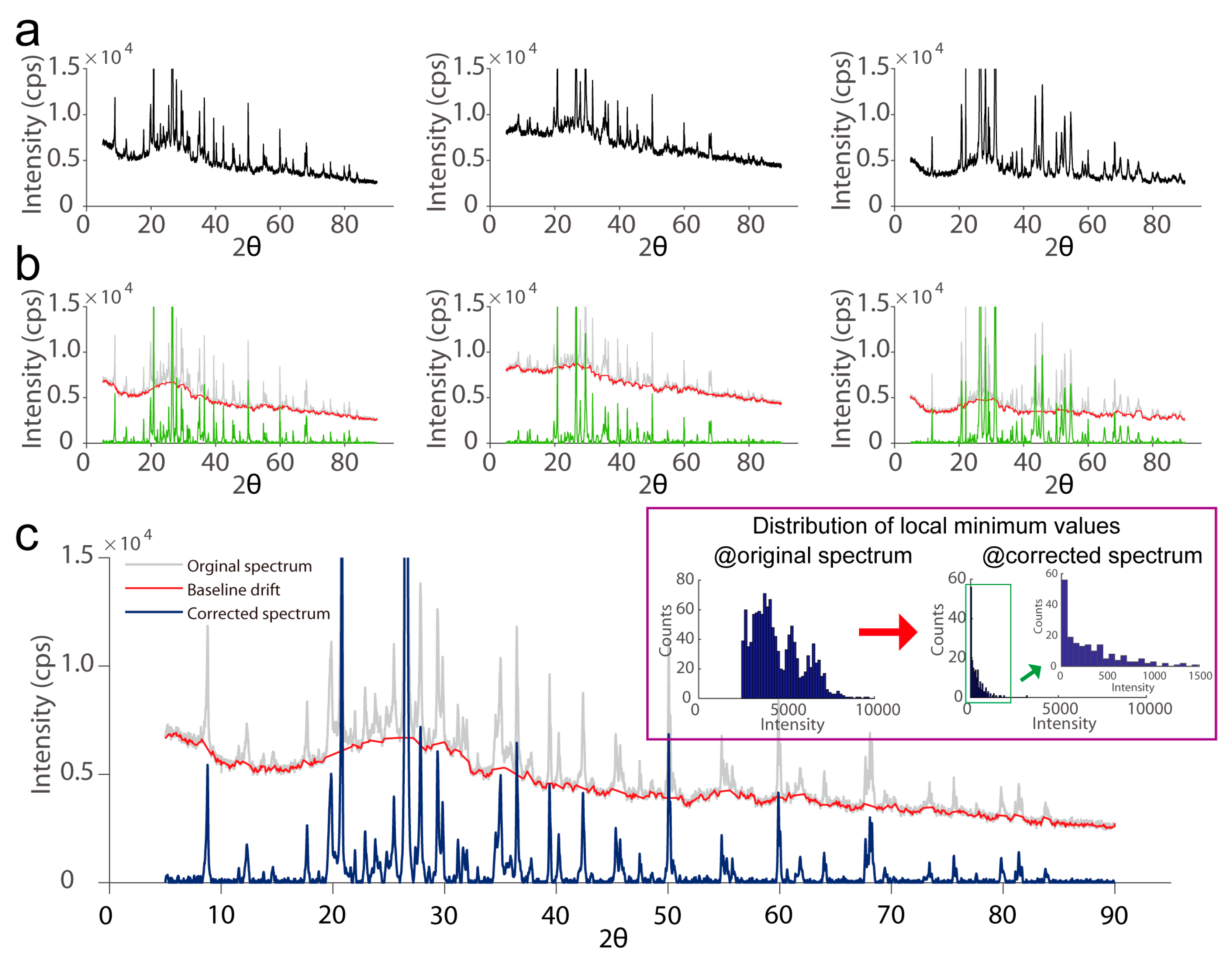
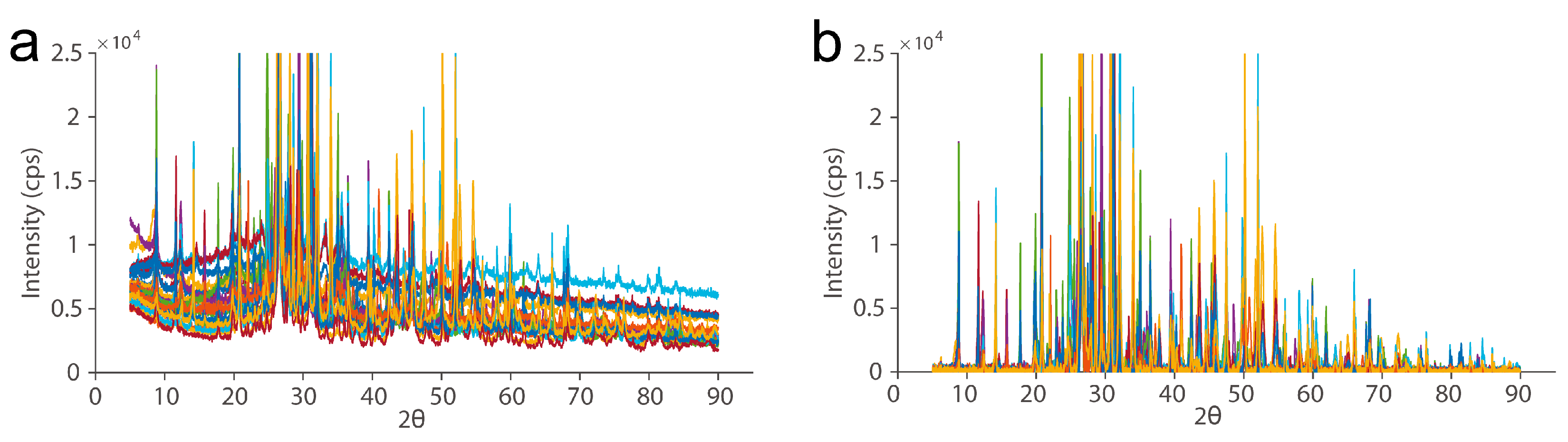
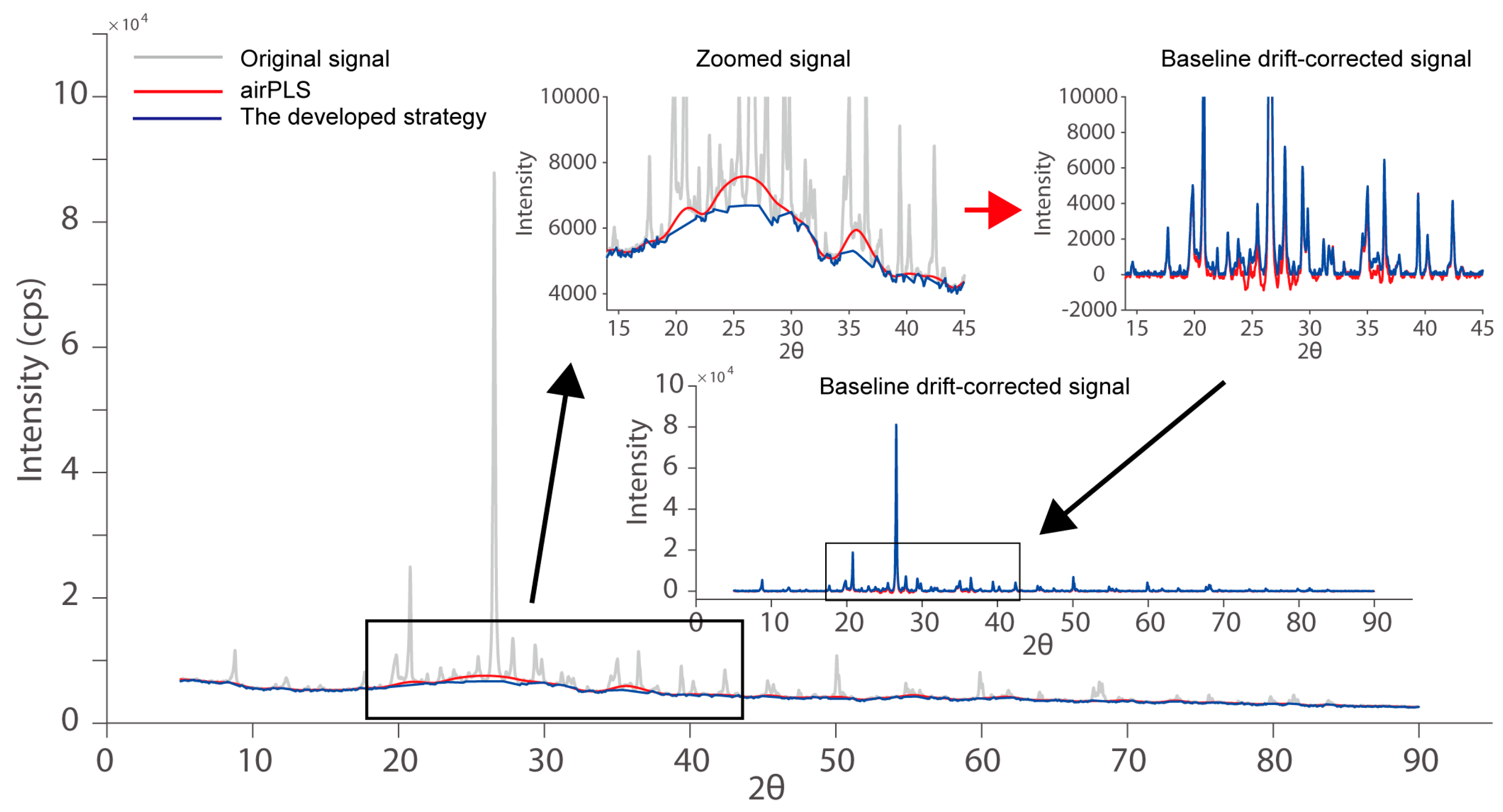
3.2. Performance in Addressing Various Kinds of Baseline Drift in the XRD Spectrum

In the routine analysis of painted pottery samples, various types of sample matrices can be obtained during archaeological excavations, leading to baseline drift that varied dramatically across samples in the case of XRD analysis. To demonstrate the capability of our method to deal with various kinds of baseline drift in the analyzed signal, we provided three types of baseline drift in the ancient potteries in Figure 3a. In the left column of Figure 3a, the baseline drift floated in the front part of the spectrum. Conversely, the baseline drift linearly decreased in the right part of the signal. In the middle column of Figure 3a, the baseline drift decreased linearly from the beginning to the end part of the signal. Moreover, a slight upward float can be found within the 2θ range of 20 to 30. A comparison of the spectra between the first and second columns in Figure 3a indicated a total increment of background noise in the latter one, which may increase the complexity of baseline drift correction. With respect to the right column of Figure 3a, the baseline drift appeared as a horizontal line in the right part of the spectrum (2θ > 40), with an exception in the zone with 2θ < 40.
The results of baseline drift correction for the spectra in Figure 3a are shown in Figure 3b, where the estimated baseline drift and the corrected signals are marked with red and green lines, respectively. After removing local minima belonging to XRD peaks, the local minimum values in the signal can briefly reflect the baselines in each sample. The corrected signals without baseline drift can then be obtained for analysis. The results in Figure 3b further confirmed the reasonability of using local minimum values in the signal for performing baseline drift correction in the XRD analysis.
Figure 3c provides a detailed illustration of the baseline drift correction by using the spectrum in the middle plot of Figure 3a. The local minimum values in the overlapped XRD peaks can be efficiently filtered out with the developed outlier detection algorithm. Therefore, baseline drift can be reasonably performed with the maintained ones. Notably, we preferred to use simple linear interpolation instead of complex curve fitting for implementing baseline drift correction because the former can maximally avoid the resorting problem during correction. Evidently, the baseline drift problem in the original XRD spectrum was resolved, and the XRD peaks can be maintained simultaneously.
The distribution characteristics of local minimum values in the signal of Figure 3c were studied to determine whether the baseline drift in the XRD spectrum was efficiently corrected. Notably, all local minimum values in the spectra were extracted according to Equation (2), and those whose intensity was below 10,000 were provided in the inserted plot. The local minimum values in the original XRD spectrum were distributed with several local apices along the intensity axis (x-axis). In this case, determining a noise level to accurately extract XRD peaks for performing such as mineralogical analysis was difficult. However, with the aid of the developed strategy, the local minimum values were distributed within a relatively narrow range (below 1000) along the intensity axis. In this case, analysts can readily perform XRD peak extraction by setting a value as the level of background noise.
The results of baseline drift correction for all analyzed samples are shown in Figure 4. Figure 4a depicts the original XRD spectra of 22 ancient colored pottery samples. The baseline drift relatively differed across samples, which may distort accurate sample grouping. With the aid of the developed strategy, one can automatically perform baseline drift correction for each sample to obtain high-quality XRD spectra for sample analysis (Figure 4b). Notably, after removing baseline drifts in all samples, the noise level was almost identical among the samples.
Variance explained by the principal components (PCs) was first investigated, and the results corresponding to red and white potteries were shown in Figures S3 and S4, respectively. It can be found clearly that the largest variance explained by PC1 is in the original XRD spectra without treatment (left columns of Figures S3 and S4). By contrast, the results for the XRD spectra with baseline drift correction suggested that the baseline drift can be successfully removed from the loading profile of PC1, and meanwhile, unwanted variance in baseline drift can be eliminated, resulting in the decrement of explained variance by PC1. The mean-centering treatment was used for further demonstration, as a part of the biased signal from baseline drift can be removed. It can be found from the middle columns of Figures S3 and S4 that the variance explained by PC1 reduced by more than 40% for the original XRD spectra after mean-centering treatment. With the aid of baseline correction, the reduction in explained variance by PC1 was about 25%. Moreover, the values of explained variance by PC1 are larger for the data with baseline drift correction than those without correction.
Another interesting phenomenon can be found in the right column of both Figures S3 and S4; in the case of autoscaling, the baseline drift problem in the original XRD spectra seemed to be enhanced greatly when compared with the mean-centering treatment. In this case, the variance explained by PC1 increased again. With respect to the XRD spectra with baseline drift correction, the autoscaling can place equal weights for all variables in each XRD spectrum. In this case, the effect of random variables was relatively reinforced so that, theoretically, the variance explained by PC1 decreased to a smaller value when compared with the mean-centering treatment, which can be clearly found in Figures S3 and S4. These results implied that the effect of baseline drift can be resolved by our strategy so analysts can focus on the accurate grouping of ancient colored pottery samples from different periods or locations.

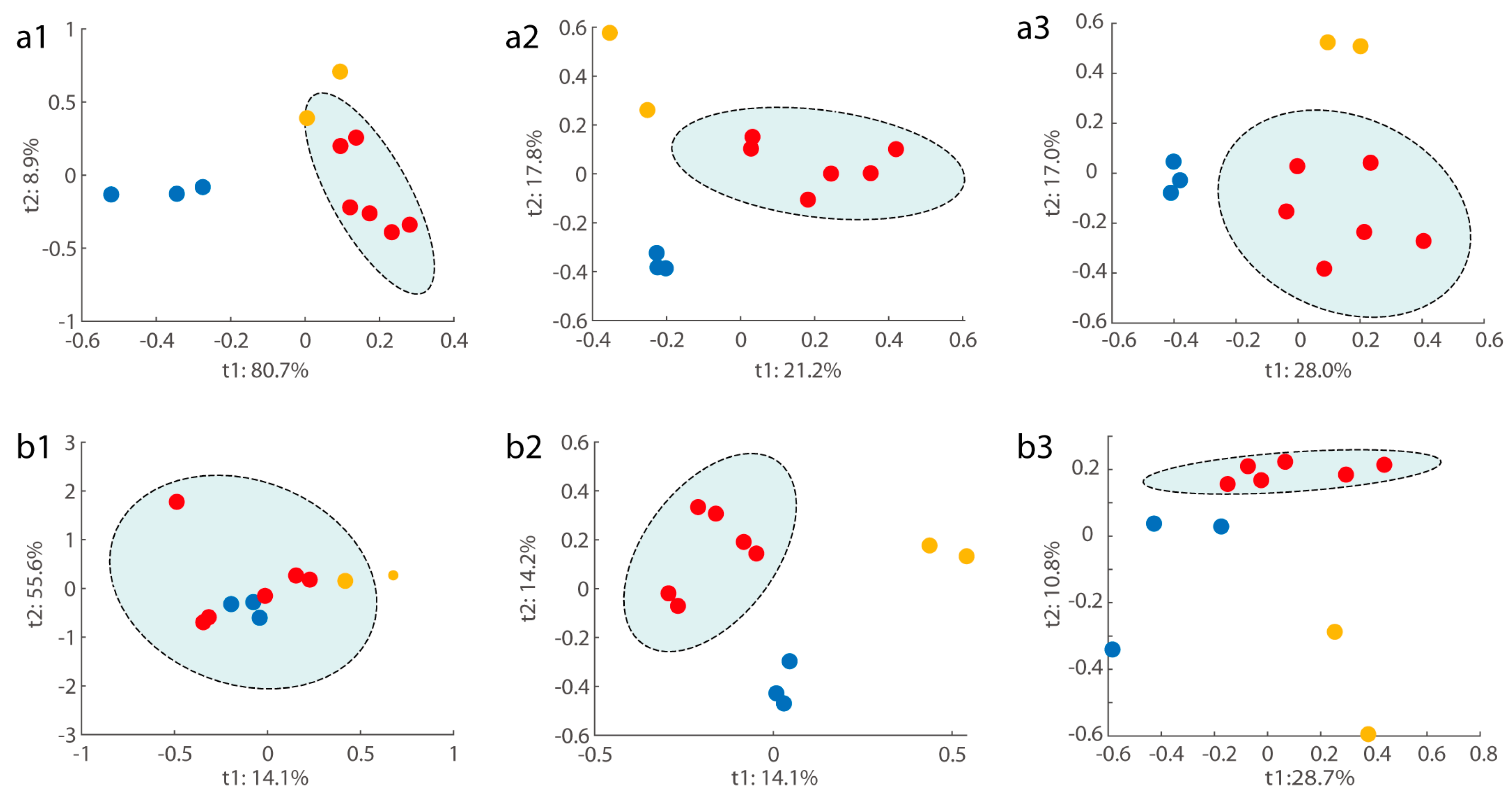
3.3. Chemometric Analysis of Ancient Painted Pottery

Since the period for which the artifacts are dated is long, it can be expected that some changes in the production technology may be varied. In this work, we focused on the separation of pottery samples from different zones or dynasties by using the baseline drift-corrected XRD spectrum, which may be the first study in this aspect. A 4251 × 11 matrix was obtained for analysis with 4251 data points in each spectrum, and 11 was the number of white or red potteries. PCA was initially performed based on the XRD spectra, and the results are shown in Figure S5. Notably, pretreatment with mean centering was employed for both the original and the corrected XRD spectra. The original XRD spectra classified potteries from Zhongwei City and Guyuan City clearly. After the removal of baseline drift, however, potteries from Zhongwei City cannot be separated from those from Guyuan City. The slight difference may lie in the fact that baseline drift cannot be eliminated efficiently by the mean-centering treatment (see Figure S3). PCA was also performed using the mineralogical and element compositions in Table S1 as the benchmark, and results were shown in the right column of Figure S5. It can be found that the potteries cannot be separated either, which was briefly consistent with those with baseline drift correction. The analysis of white potteries indicated that they cannot be separated based on either dynasty or location, which can be found from the XRD spectra with and without baseline drift correction in Figure S5. Consistent results can be also found from the PCA based on the mineralogical and element compositions in Table S2. In fact, pretreatment with autoscaling was also performed, and the results are shown in Figure S6. It can be found that similar results can be also obtained for the studied potteries, except that the variance explained by the first two PCs was higher in the original XRD spectra. A very possible reason for this may be that the problem of baseline drift was enhanced after autoscaling (see Figures S3 and S4).
The supervised classification method, PLS-DA, was used for sample grouping, and the results are shown in Figure 5. Notably, data treatment of the mean center and normalization were used for XRD spectra. The left column of Figure 5 shows the sample-grouping results from the original XRD spectra. These samples cannot be classified because the ellipses (<95% confidence level) of the samples corresponding with Zhongwei City partially covered the samples from the other groups. Specifically, the white materials from Guyuan and Zhongwei seriously overlapped (Figure 5(a1,b1)).
Conversely, sample grouping results in the middle column of Figure 5a indicated that samples from different cities and dynasties can be clearly separated, indicating the success of baseline drift correction. The samples from Guyuan (blue circles) and Zhongwei (red and yellow circles) cities were clearly divided into different parts in the plots of Figure 5(a2,b2). With respect to the samples from the Tang (yellow circles) and Han (red) dynasties in Zhongwei City, they can be properly separated. Given the very rare ancient painted pottery studied in this work, prediction was not performed for the limited sample number. The results in Figure 5 suggested that with efficient baseline drift correction, ancient painted potteries can be discriminated against using the entire XRD spectrum in an untargeted manner.
To demonstrate the success of the developed strategy, mineralogical and EDS analyses were manually performed, and the results are shown in Tables S1 and S2. Sample grouping results for the red and white materials are shown in Figure 5(a3,b3), respectively. The developed XRD spectrum-based untargeted strategy can obtain almost identical sample grouping results with manual resolution. With the aid of the local minimum-based correction algorithm, baseline drift can be reasonably corrected, and samples from different zones and dynasties can be satisfactorily separated. The developed XRD spectrum-based untargeted strategy had the great advantage of not needing manual deconvolution for mineralogical analysis, so the risk of incorrect deconvolution results can be greatly avoided.

3.4. Brief Comparison with State-of-the-Art Methods

The requirement of baseline drift correction was not limited in the XRD analysis. In some signal analysis fields such as chromatography and NMR, a number of state-of-the-art algorithms [20,22,23] have been developed as well. However, their applications in XRD spectroscopy are not reported publicly. Here, a brief comparison was provided. The famous airPLS of Zhang was introduced [23] for XRD spectrum analysis for the first time. We selected a sample to provide an illustration, and the baseline drift correction results from the developed strategy and airPLS are shown in Figure 6. It must be noted that a single sample analysis cannot provide a statistical evaluation of the performance of a method. The estimated baseline from the airPLS was almost identical to that of the developed strategy. The Pearson coefficient of estimated baselines from the two methods was 0.9908. The slight difference lay within the zone ranging from 15 to 45, where overlapped XRD peaks were present in the analyzed signal. airPLS trended to overfit the baseline drift for peaks without baseline correction. Conversely, results from the developed strategy may be more acceptable for baseline drift correction of overlapped XRD peaks, indicating that the developed algorithm may be valuable for XRD data analysis.
The above-mentioned results demonstrated that the developed local minimum value-based strategy can efficiently address the baseline drift problem in the XRD spectrum. This strategy can benefit the XRD spectrum-based untargeted strategy for the classification of ancient painted pottery. Evidently, ancient painted pottery from the Han and Tang dynasties can be successfully separated after reasonable baseline drift correction by using the developed strategy. Meanwhile, their locations can be accurately classified. The developed baseline drift correction method was also insensitive to initialized parameters, i.e., cutoff value for signal-to-noise ratios and moving window size. These features enabled data analysis to be performed almost automatically in routine work. To benefit the ancient painted pottery analysis, our strategy was implemented in a GUI, which can be obtained from the authors.

4. Conclusions

We proposed a new automatic XRD spectrum-based untargeted strategy for the accurate classification of ancient painted pottery from different dynasties and locations. To eliminate the influence of baseline drift in the analyzed signal, a local minimum value-based baseline drift correction algorithm was specifically designed. The developed strategy can automatically and efficiently estimate baseline drift in the XRD spectrum and thus provide accurate classification results for ancient painted pottery. Potteries from the Han and Tang dynasties in the cities of Guyuan and Zhongwei, China, were used to demonstrate the success of the developed strategy, and the results indicated that it could provide a new solution for ancient sample analysis.

Supplementary Materials

The following supporting information can be downloaded at: https://www.mdpi.com/article/10.3390/chemosensors12040064/s1, Figure S1: Typical potteries collected in this work. The upper plot is a red pottery, where as the lower one is a white pottery; Figure S2: Matlab GUI of AntDAS-XRD; Figure S3: Variance and loading from XRD spectra of red pottery with and without baseline-drift correction. First row show variance explained by principal components. Second row show loading plot corresponding to the PC1. Left, middle, and right columns were spectra untreated, mean-centering, and autoscaling, respectively; Figure S4: Variance and loading from XRD spectra of white pottery with and without baseline-drift correction. First row show variance explained by PCs. Second row show loading plot corresponding to the PC1. Left, middle, and right columns were spectra untreated, mean-centering, and autoscaling, respectively; Figure S5: Sample clustering based on PCA. Left column: clustering of potteries based on original XRD spectra (mean-centering treatment). Middle column: clustering of potteries based on original XRD spectra (mean-centering treatment). Right column: clustering of potteries based on data of Table S1 and S2. Autoscaling treatment was employed for the data of Table S1 and S2. Blue circles represent samples from the Guyuan city of the Han dynasty. Red circles are samples from the Zhongwei city of the Han dynasty. Yellow circles is samples from the Zhongwei city of the Tang Dynasty; Figure S6: Sample clustering based on PCA. Left column: clustering of potteries based on original XRD spectra (autoscaling treatment). Middle column: clustering of potteries based on original XRD spectra (autoscaling treatment). Right column: clustering of potteries based on data of Table S1 and S2. Autoscaling treatment was employed for the data of Table S1 and S2. Blue circles represent samples from the Guyuan city of the Han dynasty. Red circles are samples from the Zhongwei city of the Han dynasty. Yellow circles is samples from the Zhongwei city of the Tang Dynasty; Table S1: Analysis results for the red pigments of ancient potteries; Table S2: Analysis results for the white pigments of ancient potteries.

Author Contributions

Conceptualization, J.-J.S., Y.-Y.W. and Y.-J.Y.; funding acquisition, J.-J.S.; investigation, Y.-Y.W. and F.-L.M.; project administration, W.-C.T. and J.-N.W.; software, Y.-J.Y.; writing—original draft, Y.-Y.W. and J.-N.W.; writing—review and editing, J.-J.S., F.-L.M. and Y.-J.Y. All authors have read and agreed to the published version of the manuscript.

Funding

The authors gratefully acknowledge the financial support of the National Natural Science Foundation of China (Grant Nos. 22378214) and the Natural Science Foundation of Ningxia (2021AAC03438, 2023AAC05038).

Data Availability Statement

Data are contained within the article and Supplementary Materials.

Conflicts of Interest

The authors declare no conflicts of interest.

References

  1. Shalvi, G.; Shoval, S.; Bar, S.; Gilboa, A. Pigments on Late Bronze Age painted Canaanite pottery at Tel Esur: New insights into Canaanite–Cypriot technological interaction. J. Archaeol. Sci. 2020, 30, 102212. [Google Scholar] [CrossRef]
  2. Jones, R. The Decoration and Firing of Ancient Greek Pottery: A Review of Recent Investigations. Adv. Archaeomater. 2021, 2, 67–127. [Google Scholar] [CrossRef]
  3. Buravlev, I.Y.; Gelman, E.I.; Lapo, E.G.; Pimenov, V.A.; Martynenko, A.V. Three-colored Sancai glazed ceramics excavated from Bohai sites in Primorye (Russia). J. Archaeol. Sci. Rep. 2022, 41, 103346. [Google Scholar] [CrossRef]
  4. Gajić-Kvaščev, M.; Bikić, V.; Wright, V.J.; Radosavljević Evans, I.; Damjanović-Vasilić, L. Archaeometric study of 17th/18th century painted pottery from the Belgrade Fortress. J. Cult. Herit. 2018, 32, 9–21. [Google Scholar] [CrossRef]
  5. Li, Y.; Wu, S.; Yang, J. Multi-analytical investigation of decorative coatings on Neolithic Yangshao pottery from Ningxia, China (4000–3000 BCE). J. Eur. Ceram. Soc. 2021, 41, 6744–6755. [Google Scholar] [CrossRef]
  6. Wu, X.; Ji, F.; Zhang, X.; Wang, F.; Feng, F.; Lu, Q.; Zhao, S.; Zhang, Y.; Wang, C.; Huang, F.; et al. Geochemical evidence reveals a long-distance trade of white pottery in Neolithic China 5000 years ago. J. Archaeol. Sci.-Rep. 2022, 44, 103533. [Google Scholar]
  7. Ortega, L.A.; Zuluaga, M.C.; Alonso-Olazabal, A.; Murelaga, X.; Alday, A. Petrographic and geochemical evidence for long-standing supply of raw materials in neolithic pottery (mendandia site, spain). Archaeometry 2010, 52, 987–1001. [Google Scholar] [CrossRef]
  8. Bayazit, M.; Adsan, M.; Genç, E. Application of spectroscopic, microscopic and thermal techniques in archaeometric investigation of painted pottery from Kuriki (Turkey). Ceram. Int. 2020, 46, 3695–3707. [Google Scholar] [CrossRef]
  9. Bruni, S.; Guglielmi, V.; Della Foglia, E.; Castoldi, M.; Bagnasco Gianni, G. A non-destructive spectroscopic study of the decoration of archaeological pottery: From matt-painted bichrome ceramic sherds (southern Italy, VIII–VII B.C.) to an intact Etruscan cinerary urn. Spectrochim. Acta A 2018, 191, 88–97. [Google Scholar] [CrossRef]
  10. Copley, M.S.; Bland, H.A.; Rose, P.; Horton, M.; Evershed, R.P. Gas chromatographic, mass spectrometric and stable carbon isotopic investigations of organic residues of plant oils and animal fats employed as illuminants in archaeological lamps from Egypt. Analyst 2005, 130, 860–871. [Google Scholar] [CrossRef]
  11. Ichikawa, S.; Matsumoto, T.; Nakamura, T. X-ray fluorescence determination using glass bead samples and synthetic calibration standards for reliable routine analyses of ancient pottery. Anal. Chem. 2016, 8, 4452–4465. [Google Scholar] [CrossRef]
  12. Szalóki, I.; Braun, M.; Van Grieken, R. Quantitative characterisation of the leaching of lead and other elements from glazed surfaces of historical ceramics. J. Anal. At. Spectrom. 2000, 15, 843–850. [Google Scholar] [CrossRef]
  13. Weiss, C.; Köster, M.; Japp, S. Preliminary Characterization of Pottery by Cathodoluminescence and SEM–EDX Analyses: An Example from the Yeha Region (Ethiopia). Archaeometry 2016, 58, 239–254. [Google Scholar] [CrossRef]
  14. Aoyama, H.; Yamagiwa, K.; Fujimoto, S.; Izumi, J.; Ganeko, S.; Kameshima, S. Non-destructive elemental analysis of prehistoric potsherds in the southern Ryukyu Islands, Japan: Consideration of the pottery surface processing technique in the boundary region between the Japanese Jōmon and Neolithic Taiwan. J. Archaeol. Sci. Rep. 2020, 33, 102512. [Google Scholar] [CrossRef]
  15. Liu, Y.; Yang, F.; Wang, L. Exploratory research about the selective cleaning of calcium sulfate sediments on archaeological potteries. New J. Chem. 2020, 44, 7412–7416. [Google Scholar] [CrossRef]
  16. Rončević, S.; Svedružić, L.P.; Štrukil, Z.S.; Čakširan, I.M. Determination of chemical composition of pottery from antic Siscia by ICP-AES after enhanced pressure microwave digestion. Anal. Chem. 2012, 4, 2506–2514. [Google Scholar] [CrossRef]
  17. Hunt, A.M. The Oxford Handbook of Archaeological Ceramic Analysis; Oxford University Press: Oxford, UK, 2017. [Google Scholar]
  18. Heimann, R.B.; Maggetti, M. Ancient and Historical Ceramics; Schweizerbart Science Publishers: Stuttgart, Germany, 2014. [Google Scholar]
  19. Gliozzo, E. Ceramic technology. How to reconstruct the firing process. Archaeol. Anthropol. Sci. 2020, 12, 260. [Google Scholar] [CrossRef]
  20. Zhang, Q.; Li, H.; Xiao, H.; Zhang, J.; Li, X.; Yang, R. An improved PD-AsLS method for baseline estimation in EDXRF analysis. Anal. Chem. 2021, 13, 2037–2043. [Google Scholar] [CrossRef]
  21. Fu, H.Y.; Li, H.D.; Yu, Y.J.; Wang, B.; Lu, P.; Cui, H.P.; Liu, P.P.; She, Y.B. Simple automatic strategy for background drift correction in chromatographic data analysis. J. Chromatogr. A 2016, 1449, 89–99. [Google Scholar] [CrossRef]
  22. Baek, S.-J.; Park, A.; Ahn, Y.-J.; Choo, J. Baseline correction using asymmetrically reweighted penalized least squares smoothing. Analyst 2015, 140, 250–257. [Google Scholar] [CrossRef]
  23. Zhang, Z.-M.; Chen, S.; Liang, Y.-Z. Baseline correction using adaptive iteratively reweighted penalized least squares. Analyst 2010, 135, 1138–1146. [Google Scholar] [CrossRef] [PubMed]
Figure 1. Graphical illustration of the developed baseline drift correction algorithm in XRD spectrum. (a) Detailed steps of baseline drift correction. (b) Corresponding baseline drift-corrected spectrum. Green circles in (a) mark the outliers of local minimum values.
Chemosensors 12 00064 g001
Figure 2. An investigation of the effects of initialized parameters on the quality of baseline-drift correction. (a) Baseline drift correction results with various cutoff values of n/ε in the first-order derivation, and (b) their similarity to the original spectrum. (c) Baseline drift correction results with various moving window sizes, and (d) their similarity to the original spectrum.
Chemosensors 12 00064 g002
Figure 3. A quality evaluation of the developed baseline drift correction. (a) Various types of baseline drift problems in the original XRD spectra. (b) Estimated baseline drift with the developed strategy (red lines) and the corresponding correction results (greed lines). (c) Enlarged baseline drift correction to show the distribution characteristics of the local minimum values before and after baseline drift correction (inserted plot).
Chemosensors 12 00064 g003
Figure 4. Baseline drift correction results for painted ancient pottery samples: (a) original XRD spectra and (b) XRD spectrum with baseline drift correction.
Chemosensors 12 00064 g004
Figure 5. PLS-DA comparison of the classification of ancient pottery samples with and without baseline drift correction. (a1)–(a3) Sample grouping results on the basis of red pigments of potteries. (b1)–(b3) Sample grouping results for white pigments of potteries. Plots of (a1,b1) in the left column show results with the original XRD spectrum, whereas (a2,b2) in the middle column show results from the XRD spectrum with baseline drift correction. (a3,b3) show sample grouping results by combining data from mineralogical and EDS analyses. Blue circles represent samples from Guyuan City of the Han dynasty. Red circles are samples from Zhongwei City of the Han dynasty. Yellow circles denote samples from Zhongwei City of the Tang dynasty.
Chemosensors 12 00064 g005
Figure 6. A brief comparison of the developed baseline drift correction strategy with the airPLS.
Chemosensors 12 00064 g006
Disclaimer/Publisher’s Note: The statements, opinions and data contained in all publications are solely those of the individual author(s) and contributor(s) and not of MDPI and/or the editor(s). MDPI and/or the editor(s) disclaim responsibility for any injury to people or property resulting from any ideas, methods, instructions or products referred to in the content.

