Abstract
A device was developed to study the evolution of fluorescence spectra as a function of time. A previously designed fluorimeter based on the diode array mini-spectrometer CM12880MA was used. The control and measurement were carried out by programming a SAM21D microcontroller. Considerations regarding the optimization of acquisition speed, memory, and computer interface have been analyzed and optimized. As a result, a very versatile device with great adaptability, reduced dimensions, portability, and a low budget (under EUR 500) has been built. The sensitivity, controlled by the integration time of the photodiodes, can be adjusted between 10 µs and 20 s, thus allowing sampling times ranging from 10 ms to more than 10 h. Under these conditions, chemical rate constants from 20 s−1 to 10−8 s−1 can be experimentally determined. It has a very wide operating range for the kinetic rate constant determination, over six orders of magnitude. As proof of the system performance, the oxidation reaction of Thiamine in a basic medium to form fluorescent Thiochrome has been employed. The evolution of the emission spectrum has been followed, and the decomposition rate constant has been measured at 2.1 × 10⁻³ s−1, a value which matches those values reported in the literature for this system. A Thiochrome calibration curve has also been performed, obtaining a detection limit of 13 nM, consistent with literature data. Additionally, the stability of Thiochrome has been tested, being the photo-decomposition rate constants 1.8 × 10⁻⁴ s−1 and 3.0 × 10⁻⁷ s−1, in the presence and absence of UV light (365 nm), respectively. Finally, experiments have been designed to obtain, in a single measurement, the values of both rate constants: the formation of Thiochrome from Thiamine and its photo-decomposition under UV light to a non-fluorescent product. The rate constant values obtained are in good agreement with those previously obtained through independent experiments under the same experimental conditions. These results show that, under these conditions, Thiochrome can be considered an unstable intermediate in a chemical reaction with successive stages.
1. Introduction
This study focusses on the development of a system capable of performing fluorokinetics analysis by using a Micro-Electro-Mechanical System (MEMS)-based mini-spectrometer, adapted as a fluorimeter, controlled and operated by a microcontroller. The device is programmed under the open-source software declaration (FOSS) [1]. As an initial application, a kinetic study of the evolution of the fluorescent product produced in the oxidation of Thiamine (TA) has been carried out.
The application of the phenomenon of fluorescence continues to be a subject of current interest in scientific publications. There are numerous applications in the literature for the development of fluorescent markers, which have applications in diverse fields, ranging from the development of fluorescent protein-based biosensors that allow for the monitoring of physiological processes [2,3,4] to the monitoring and detection of contamination in environmental water, food samples, and pesticide residues [5,6,7]. Some of these applications use fluorokinetics methods combined with chemometrics for the detection of cancer toxins [8]. The worldwide economic impact relative to fluorescent detection devices is really important in many industrial applications. Thus, the food industry is projected to reach EUR 20 billion in 2025 [9], pesticide and water pollutant analyses are estimated to be worth about EUR 1.5 billion annually [10], and water management is expected to reach approximately EUR 4.5 billion in 2027 [11,12].
Kinetic fluorometry is also used in the study of photosynthesis using a technique called delayed fluorescence using far-red light for excitation. Response times typically range from milliseconds to several minutes [13]. Recently, strategies have been developed for imaging applications of fluorescent probes for ATP [14], which use longer excitation and emission wavelengths that allow for detection in deep biological samples. In this field, a very promising fluorescent probe (Bio-SiR) has been presented for the real-time imaging of ATP in cancer cells, which is a si-rhodamine-based fluorophore [15]. It is presented as the first tumor-targeting (near IR) molecule fluorescent probe for endogenous ATP imaging in real time for tumor-bearing mice.
The basic instrument (hardware) and a proposed program (software) for kinetic measurements of fluorescence spectra are discussed in this work. The development is founded mainly on studies [16,17] and the references therein. Both papers constitute the fundamentals of the proposed system, the former focusing mainly on hardware requirements and the latter on software basics. The initial advantages are obviously the high reproducibility and sensitivity already demonstrated, the low budget, and portability. A new step has been taken to develop an inexpensive, portable, and simple diode array kinetic fluorimeter. Thus, it is possible to take advantage of the benefits and minimize the drawbacks pointed out in the bibliography (open source, stability, sensitivity, reliability, cost, etc.). More specifically, it is necessary to develop a system capable of recording fluorescence spectra with an acquisition frequency as wide as possible, minimizing difficulties derived from the slowness in obtaining and storing the measured spectra. The previous paper proposes the use of a development board based on the ATSAMD21G18 [18] microcontroller for the acquisition and control of the Hamamatsu CA12880MA [19] diode array spectrometer. The developed software was applied for stationary measurements of fluorescent samples, spectra, and static quantitative determinations. The time variable is only employed for the control of the spectrometer lines and the time that excitation light is on, allowing a very large sensitivity range. The second paper established the basis for both the external parameter verification (controlled by using a spreadsheet) and for the precise time control during the measurement. The add-on macro software embedded in the spreadsheet for the control of the system has been kept and is based on Parallax Data Acquisition Tools Release 2B [20] but using a newer, more versatile and user-friendly version [21].
To verify the usefulness and reliability of the proposed device, vitamin B1 or Thia-mine (TM) has been chosen as a starting compound acting as a fluorescent precursor. TM is an essential vitamin for human beings, the deficiency of which produces the well-known “beriberi” syndrome. It mainly affects the nervous and cardiovascular systems when blood levels are in the range of 9–14 nmol/L [22]. In the literature, many analytical methods can be employed for TM investigations, such as colorimetric, fluorescence, electrochemical, chemiluminescence, electrochemiluminescence, HPLC, optical detection by using nanoparticle methods, etc. [23]. The determination of TM and related compounds via fluorescence has been widely described in the literature for more than 80 years [24]. Its sensitivity and specificity have been used to develop methods for the determination of other compounds that react with Thiamine [25], and even specific detectors have been developed for its determination [26,27]. Ryan et al. [28,29] developed and exhaustively described a kinetic method for the analytical determination of TM, which is the methodological basis for the present work. Their methodology is so well founded that it has been the subject of undergraduate teaching material [30]. Even more recently, there has been some interest in the study of the oxidation of TM to form fluorescent compounds, such as Thiochrome (TC) [23,31,32]. The kinetic behavior of these compounds provides a suitable framework for testing the versatility and limits of the fluorokinetic device presented in this study. It offers many advantages in this field, such as a high sensitivity for fluorescence measurements, fast acquisition times, low cost, great portability, and full spreadsheet integration for experimental data analysis. The results are compared with those published in the literature to evaluate the system’s overall performance.
2. Materials and Methods
2.1. Experimental
Analytical-grade chemicals were purchased from Sigma Aldrich: Thiamine hydrochloride (CAS 67-03-8), Na3PO4·12H2O (CAS 10101-89-0), Na2HPO4 (CAS 7558-79-4), sodium hydroxide (CAS 1310-73-2), hydrochloric acid (CAS 7647-01-0) and mercury (II) chloride (CAS 7487-94-7). Water was purified using a Millipore system (Milli-Q Reference model), and all measurements were performed at 22 ± 2 °C. Hellma Suprasil precision quartz cells (type 101-QS) with a light path of 10 mm were used for experimental measurements.
Figure 1 shows a picture of the proposed device with the main components of the system. As can be noted, it is a portable device with small dimensions (120 mm × 80 mm × 60 mm), with an overall weight of 0.4 Kg. As excitation sources, it contains an LED (365 nm) and a laser diode (405 nm), which is included in the GroupGets board v1. The Hammatsu C12880MA has 15 nm of spectral resolution and a wavelength range from 340 to 850 nm, allowing one to acquire 288 spectrum points. The cell compartment has a standard size of 10 mm wide.
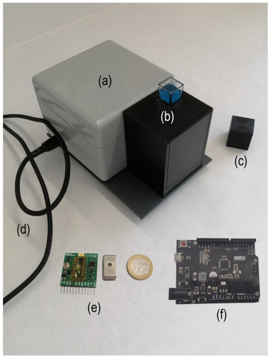
Figure 1.
Image of the proposed device showing the main components of the system: (a) fluorimeter box, (b) cell and mirrors compartment, (c) cell cap, (d) USB connection cable, (e) GroupGets breakout (v.1), Hamamatsu C12880MA spectrometer and (f) microcontroller ATSAMD21G18 board. The Euro coin is included for size reference.
2.2. ATSAMD21G18 Microcontroller Hardware
The characteristics of the microcontroller selected in terms of processing speed, clock frequency (CLK), and internal 32 kB SRAM memory are interesting. However, two major difficulties were encountered at the beginning. Firstly, the process to obtain the internally stored data, using the common read mode, was particularly slow. Secondly, the available microcontroller memory is limited to storing the different spectra for a kinetic process. Furthermore, in the measurement process, there was no possibility to reduce the noise level by averaging without sacrificing its speed. Strategies for accelerating data acquisition, averaging, and memory optimization will be explained in the following sections.
More detailed information on these aspects can be found in the Supplementary Materials.
2.3. Speeding up the Software Code for “analogRead”
Despite all the advantages mentioned in relation to the selected microcontroller, there was an added difficulty with the speed of processing the “analogRead” instruction, when the default compilation of the high-level language is employed. This instruction uses the microcontroller analog-to-digital converter (ADC) and is essential for reading/storing the light intensity values for each wavelength. A comparative speed study of the three microcontrollers (UNO, 2560, and ZERO) using the compiled instruction was performed to obtain a complete spectrum of 288 wavelength (WL) data. The time required for the first two boards was about 37 ms, but, incredibly, for the ZERO board, it was about 250 ms. Undoubtedly, the compiler used to translate the instruction for this board was inefficient and, with this timing, the use of the direct compiled instruction for ZERO makes it useless for kinetics purposes. Fortunately, this speed issue was pointed out on different internet forums. On the Arduino forum, an example code for “speeding-up” the analog-to-digital converter (ADC) compilation was presented [33]. This code involved specific port control for the SAM21D analog-to-digital converter (more information is available in the Supplementary Materials). The time required for retrieving a whole spectrum varies from 8 ms for an average of two samples to 89 ms for an average of 64 samples. A study of the error associated with the number of averages shows that the standard deviation is lower, and the absolute error changes its sign for an average between 32 and 64 samples.
2.4. Timing Control
One of the most important advantages of microcontrollers is the precise and fast timer control. Internal timers can be set up to obtain the number of microseconds or milliseconds elapsed since they were triggered. The time required to perform a measurement process involves different tasks, and each one has its own time consumption. To perform one single measurement and control the lines of the C12880MA, this process is fully described in the previous paper. The main difference is the faster procedure described in Section 2.3. Next, the selected number of data points must be stored in the data matrix. To read a new measurement, the program checks whether the selected sample time is over. If the gap time is large enough, the program writes into Excel and plots one WL selected value to check the measurement evolution. Once the gap time is over, the sequence is repeated until it reaches the number of measurements selected. For checking purposes, those timer values can be exported to Excel by checking the ‘Debug mode’ box in the PLX-DAQ controller add-on.
A detailed description of the timing process can be found in the Supplementary Materials.
2.5. Memory Optimization
Flash EPROM and SRAM memory types are implemented in microcontrollers, each one of them depending on its characteristics, and are usually assigned a specific task. Their organization and uses are widely discussed in the Arduino Memory Guide [34]. Different alternatives for the storage of kinetic data have been considered, especially taking into account two fundamental issues: the time required for their storage and the amount of data to be stored. There are also other collateral considerations such as minimizing the cost and complexity of implementation. Although it might be thought that the amount of memory available in the microcontroller is scarce, with some optimization, it is possible to store a complete spectrum every 10 ms, using just 0.5 kB. In this way, about 50 complete spectra could be stored, without consuming the entire available SRAM memory. Nonetheless, in fluorescence measurements, the area of the spectrum corresponding to the excitation source can be neglected. This fact allows a larger number of spectra to be stored in memory. On the other hand, it is possible to store more than 10,000 points if a single WL is selected (at maximum emission). With these numbers, the decision was made to use the best option offered by ATSAMD21G18, which implies an easier, cheaper, and faster development, since it has a solid base in its hardware, regarding the spectrophotometer and the development of its software.
In addition, the optimization of the available SRAM provides a higher storage speed with a reasonable software modification effort to trim and organize the measured data spectra. Thus, a single array variable is used to store the succession of clipped spectra during a kinetic experiment, once the number of wavelengths and the total number of wavelengths to be stored are known. This array of clipped spectra for different acquisition times can be exported as a two-dimensional table with two output modes: columns containing the selected WL and rows for the selected time, or the transposed mode with time in cols/rows and WL.
More detailed information about memory optimization and organization can be found in the Supplementary Materials.
2.6. Acquisition Software PLX_DAQ
As described in previous papers, the main advantage of using PLX-DAQ software Release 2B with Excel is to read and write specific parameters via USB without having to reload the code into the microcontroller every time a parameter changes. It also allows for the storage of the results and their graphing during the measurement. Moreover, using the different checkboxes included in the PLX-DAQ, the program flow and the parameter verification and validation can be performed easily.
One possible drawback is that the use of an Excel spreadsheet is mandatory, because this spreadsheet program has fundamental RS232 input/output control procedures, compatible with USB. However, its use has been developed by PLX-DAQ with open source. Version 2.11 [21] has some additional improvements, such as the selection of the spreadsheet that interacts with the USB interface and a debug output that allows for scrutinizing possible communication problems. However, the main drawback is the strict language required to build the message syntax. Special characters, usually employed for control in the Serial communication interface, can interfere with Excel: comma, spaces, line feed, and carriage return characters. Thus, it is highly recommended to carefully read the user guide.
Figure 2 shows an Excel screenshot of the control datasheet and the PLX-DAQ add-on (orange framed) for a dummy experiment.
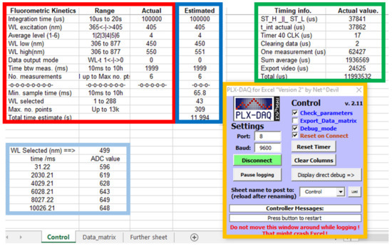
Figure 2.
Spreadsheet screenshot for the fluorokinetics control, showing input parameters (red frame), debugging information about the timing (green frame), PLX-DAQ add-on for Excel (orange frame), estimated parameters (blue frame) and actual kinetic data (cyan frame). See text for a detailed description.
2.7. Input Parameters
The variables which control the fluorokinetics experiments are related to the spectroscopic and kinetic times. In the red frame shown in Figure 2, the first column contains a brief description of the measured parameter and employed units, if applicable; the second column contains information about their valid range. The third column is used to write the desired actual values, and the fourth column contains their estimation from the actual values. The timer value (in µs) for debugging is displayed in the green frame. Their values are useful for additional testing and validation of the kinetic measurement process.
There are some interrelationships between some input parameters, and efforts have been made to maintain the maximum performance of the device (memory, time, WL). Thus, the number of kinetics points is limited by the number of WLs stored up to a maximum of 25kB. The minimum kinetic time interval is limited by the time required to operate the CA12880MA. Therefore, once the input parameters are typed in the Excel cells, it is necessary to recheck their values to verify that all device limits are matched (blue frame in Figure 2). Thus, the number of WLs to be stored is estimated from the available memory. The minimum sampling time (in milliseconds) is estimated from the internal timer values (in microseconds) with a 5% increment for safety. The exact time at which the first spectrum is recorded corresponds to half the integration time of the first measurement (see a detailed description in Supplementary Materials).
The time between measurements must be greater than the minimum sampling time. If the difference between the sampling time and the integration time is large enough (about 100 ms), it is possible to export and plot the actual kinetic data during the measurement process for a single selected WL (cyan frame in Figure 2). In this case, it is highly recommended not to operate the add-on and/or Excel during the measurement process (see Supplementary Materials for more information). Once the input parameters are set, they are checked and, if necessary, recalculated. If no errors are detected, they can be validated by marking the ‘Check_parameter’ checkbox on the add-on to proceed.
As the complete data matrix for a kinetic experiment could be very large, PLX-DAQ v2.11 allows one to select more than one datasheet to export data. Thus, one datasheet contains the control parameters, debugging, and the ADC data corresponding to the WLs selected for plotting. Other datasheets can store the entire output matrix of selected time/WL data for different experiments. This procedure can be a bit tricky initially, and special care has to be taken to avoid writing the output matrix on the control sheet or trying to read the input parameters from the data matrix sheet. Another checkbox, ‘Export_Data_matrix’, is used to minimize the possible error of writing into the wrong datasheet.
2.8. Measurement Routines
In addition to the usual code for microcontroller programming, setup and loop, several routines have been developed to efficiently perform each experiment. The most important ones are listed here (more detailed information can be found in the Supplementary Materials).
- Boosting analogRead procedure: AdcBooster(Avr_level).
- Generate n CLK pulses: F_pulse_clk3MHz(n).
- Management of the CA12880MA control lines for a single spectrum:F_readSpectrometer(Ex_L).
- Estimation of the wavelength associated from the manufacturer data:Wavelength(order).
- Computes the associated indexes according to the WL calibration data:WL_Index_Data(&w_H, &w_L, &index_H, &index_L).
- Output matrix spectra generation by row:
- create_selected_matrix_by_row(&Row_Index_L, &Row_Index_H, &actual_col, *matrix).
- Trimmed selection of the whole data matrix, including acquisition time:printDataMatrixExcel(mode, &Row_Index_L, &Row_Index_H, &N_points, &Delta_ms, off_t_ms, *Data_Matrix).
- Clean up in Excel datasheet of the parameter estimation:Clean_estimated_param().
2.9. Software Flowchart
A very simplified flowchart of the measurement process is described in Figure 3 (more detailed information can be found in the Supplementary Materials).
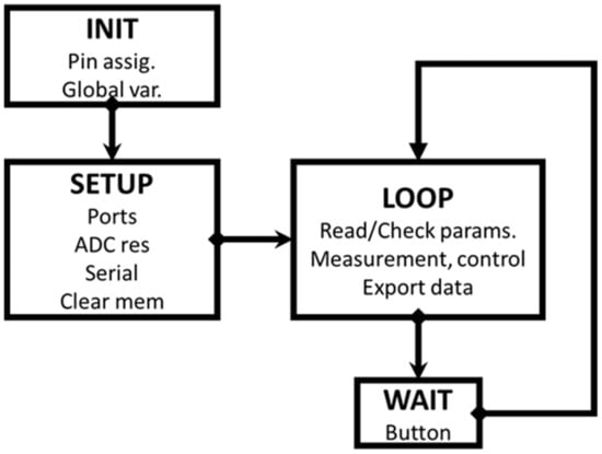
Figure 3.
Simplified scheme of the measurement process. The sequential procedure is operated by pressing the button on the fluorimeter, following the text messages from the add-on.
The device is connected via a USB port to a known COM port number. The Excel spreadsheet containing the enabled PLX_DAQ macro must use the same port value. The INIT and SETUP processes are executed only once, by writing the information in the Excel control sheet. The procedure is then controlled by pressing the device button briefly and following the instructions in the PLX-DAQ text messages. Once the measurement has been completed, special care should be taken to select the Excel sheet for data export. After exporting, select the control sheet again to be able to modify the parameters for a new measurement. This procedure is similar to the one already explained in the previous document [16,17]. The complete fluorokinetics source program, with multiple commentaries, can be obtained from the authors, upon request.
3. Results and Discussion
As a test of the versatility, capability, and accuracy of the designed fluorokinetics device, the rate of TC generation from the oxidation of TM in a basic medium has been studied.
3.1. TC Formation from TM Evolution
As mentioned in the Introduction, the reaction kinetics are very well known in the literature and are even used as an example at the higher educational level [30]. The authors recommend using Hg(II) as the oxidant agent in basic media, despite other possible indications [28,29]. TC has an emission maximum at 450 nm when excited with UV light (365 nm). Figure 4 shows the TC clipped spectrum obtained with the fluorimeter after complete oxidation of a 5 ppm TM solution in phosphate buffer (pH 12).
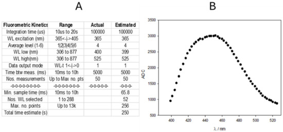
Figure 4.
(A) Screenshot of the parameters employed to obtain the emission spectrum of TC. (B) Emission spectrum obtained by Hg(II) oxidation of a 5 ppm TM solution at pH 12. Ordinate corresponds to the ADC values. No blank correction is performed.
Figure 5 shows the progress of the TM oxidation with the evolution of the TC emission spectrum. These plots can be easily obtained from the exported matrix of the radiation intensity data at the selected WLs and times during the course of the TC formation reaction. The 3D view is a striking example of the visualization of fluorokinetics measurements obtained by the designed device.
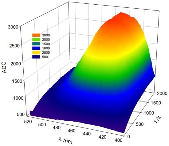
Figure 5.
Three-dimensional evolution of TC formation during Thiamine oxidation. Readings of the ADC converter of the microcontroller at different wavelengths. Experimental conditions are analogous to those described in Figure 4.
When the kinetics are relatively slow (sampling time above 2.0 s), measurements can be made by switching off the excitation light between points. However, if it is desired to obtain the rate constant at zero time, measurements have to be made at the mixing reactant early stages with short sampling times to obtain a good resolution.
Figure 6 shows the evolution of the logarithm value of the ADC reading at the wavelength of the emission maximum (450 nm). The acquisition was carried out for about half an hour. The oxidation reaction tends to be a limiting value corresponding to the amount of initial TM.
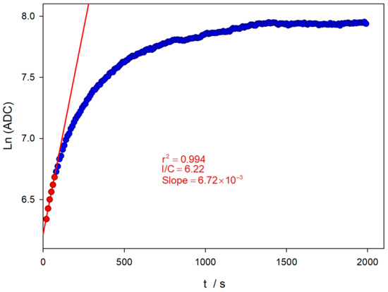
Figure 6.
Evolution of the natural logarithm of the ADC at the wavelength of the emission maximum (450 nm), until TM depletion (blue dots). Pseudo-first-order analysis for initial reaction times (red dots and line) and the experimental conditions are the same as Figure 4.
The experimental conditions applied imply that the TM oxidation reaction takes place under pseudo-first-order conditions, since the oxidant concentration is two orders of magnitude higher. At the initial reaction stages, a pseudo-first-order kinetics condition can yet be considered applicable, and a logarithmic linear relationship between the ADC value and time can be obtained, as shown in Figure 6. The evolution of the TM oxidation reaction is followed until total consumption. A sampling time of 5 s is used, and the excitation source is switched off between measurements. This avoids the possible decomposition of TC by the UV excitation light during the lengthy measurement period. A first estimation of the apparent rate constant can be obtained by the slope of the linear relationship (red line in Figure 6), obtaining a value of 6.72 × 10⁻³ s−1.
However, the value of this apparent constant, even for these early stages of the reaction, may be somewhat compromised by two effects: on the one hand, the influence of the depletion of the amount of Thiamine, and, on the other hand, the possible decomposition of TM or TC formed when the UV excitation source is kept on. For a correct analysis of the kinetic measurements, when measuring the fluorescence of the TC formed, it is necessary to perform a small modification of the equation employed by using the Guggenheim method. The reading values at the beginning and the end of the reaction have limited fixed values. At the beginning of the reaction, there is no TC, and the ADC value corresponds to a dark current value (ADC0 ≈ 400). When all the TM has been oxidized, a constant amount of TC has been formed, which will provide a limiting value of the ADClim. This value is approximately constant, since TC is quite stable in a basic medium and in the absence of light, as described in the literature [30].
Thus, the TM concentration at any time will be proportional to [ADClim − ADC]. At the beginning of the reaction, this value is [ADClim − ADC0]. Therefore, the first-order integrated kinetic equation will be:
Therefore, the representation of the first term of Equation (1) versus time has to be linear. Figure 7 shows the application of this equation to a similar experiment, as presented in Figure 6.
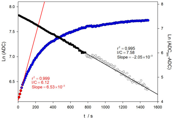
Figure 7.
Comparison of the kinetic analysis on TM oxidation in a similar experiment shown in Figure 6. The black symbols correspond to the analysis of the Guggenheim method.
As can be seen in Figure 6 and Figure 7, the analysis using the value of the logarithm of the converter directly provides a value of the oxidation rate constant close to 0.007 s−1, which is not in agreement with the literature, even using only the data corresponding to the very early stages of the reaction. In contrast, when the analysis is performed considering the limiting values, linear relationships are obtained over a wider range of reaction times. Furthermore, the value of the rate constant obtained is close to the published data, with a value of 2.02 × 10⁻³ s−1 [29].
Additionally, a new set of experiments was carried out, keeping the same conditions but using just 100 ms for a sampling time lasting 20 s. Thus, the excitation light is kept switched on during the whole measurement process. In these conditions, the obtained rate constant (1.40 × 10⁻³ s−1) is somewhat lower than the reported value. This discrepancy can be influenced by the TC photo-chemical decomposition being formed.
3.2. TC Stability in Dark Conditions
The stability of the TC solution in the absence of light was also studied. For this purpose, experiments were designed to follow the evolution of the maximum absorption value over days with sampling times of several minutes.
The fluorescence measurement is performed during intervals of 3 min (180,000 ms) for 25 h. For this process, the excitation source is switched off and it is only switched on 500 ms before the measurement. This ‘pre-lighting’ of the UV LED before the spectroscopic measurement minimizes the light jittering, improving the signal-to-noise ratio. Thus, the light is kept switched on for only 600 ms for each data point. Throughout the whole experiment, the sample is irradiated less than 300 s over one day. The first-order decay constant that can be estimated is about 3.03 × 10⁻⁷ s−1, which corresponds to a half-life of more than 26 days. In addition, several stability tests were carried out on the weakly acidic TM stock solutions kept under the protection of ambient light (amber flask). For more than one month, the fluorescence intensity results of the generated TC are reproducible in the range of 2%. This result is also in agreement with that expressed in the literature [30].
3.3. TC Calibration
Considering the stability of the TC solutions in the absence of light, a calibration of their fluorescence was performed to check linearity, detection and quantification limits. From a TC stock solution (5 ppm) stored in an amber flask, different solutions were prepared by dilution using NaOH 0.15 M as a solvent.
The spectra program described in the bibliography [16] was used for these measurements. For recording, 10 spectra were averaged, using different integration times to re-adjust the intensity signal to a reliable value. Spectra were corrected for the solvent value used as background. The calibration curve is shown in Figure 8.
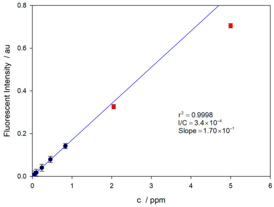
Figure 8.
Calibration curve for the TC in 0.15 M NaOH. The solutions were made in amber flasks, preventing TC photo-decomposition.
The LOD value was calculated as three-times the signal-to-noise ratio [35]. In order to evaluate the repeatability, replicate measurements were performed three times. The results show that the value of the minimum determinable concentration is LOD = 13 nM, which is in good agreement with the reported data in the literature [29]. The values corresponding to the two most concentrated solutions (red dots) have not been used for the linear regression (blue line) due to a decrease in the fluorescence intensity due to the auto-quenching effect [32].
3.4. TC Photo-Decomposition by UV Light
Both TM and TC were studied under UV light (360 nm), showing a photo-decomposition process [36,37]. For this purpose, experiments were designed where the excitation source was kept switched on during the whole measurement. In our case, TM decomposition cannot be detected using the 365 nm excitation light due to the low power of the LED source. For the TC case, a sampling time below 2 s can be used to carry out the experiments. Thus, the excitation source is kept switched on during the whole measurement. Figure 9 shows that the corrected logarithm of the ADC decreases noticeably with time in a linear relationship. The estimated first-order decay constant is 1.75 × 10⁻⁴ s−1, which corresponds to a half-life of about 1 hour. The decomposition rate is more than 600-times faster in the presence of 365 nm UV light than in darkness. The reported value for photo-decomposition by UV light at pH 12 in the literature [36], 4.2 × 10⁻⁵ s−1, is significantly lower than that reported here. However, the lamp type, power, distance, and irradiation time are significantly different from those used in this work.
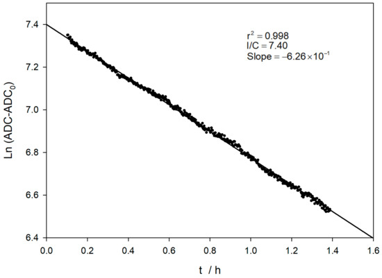
Figure 9.
Evaluation of the stability of a 5 ppm TC solution in a basic medium, in the presence of the 365 nm UV light, used as an excitation source. The experiment lasts 90 min using an integration time of less than 2 s.
In light of these results, a single fluorokinetic experiment can be designed to obtain all the kinetic parameters, that is, the TC formation from TM and the subsequent TC photo-decomposition. For this experiment, a sampling time of 1.999 s is used for 3 hours and 20 min (6000 points). In this way, there is sufficient time to observe the attenuation in the solution fluorescence that occurs due to the breakdown of the TC by the UV light.
Figure 10 shows the variation for the fluorescence signal with the time reaction of a 5 ppm solution of TM in a basic medium. Initially, TC is generated at a specific rate and subsequently degraded under UV light into a non-fluorescent compound (NF).
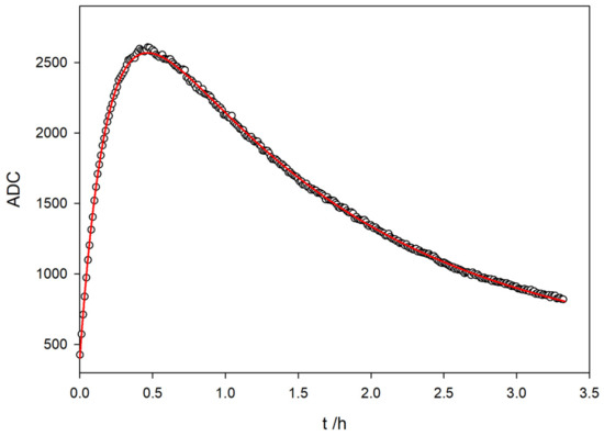
Figure 10.
Evolution of the fluorescence signal with time reaction for a 5 ppm solution of TM in basic medium. In the plot, data points are sampled every ten stored values for clarity.
The shape of the fluorescence variation with time observed in the graph closely resembles the behavior of a consecutive reaction with two different reaction rates, where TC acts as an intermediate compound:
A nonlinear least squares fitting of the AD value has been performed, using the Equation [38]:
Table 1 shows the estimated parameters and the statistical fit for the consecutive reaction. The red line in Figure 10 corresponds to the fit with the parameters from Table 1.

Table 1.
Results of the nonlinear least squares fit for the formation of TC from the oxidation of TM and its decomposition by UV light.
It can be easily checked that the constant rates found with the proposed method are in perfect agreement with those obtained for independent experiments corresponding to the formation of TC via the oxidation of TM and photochemical degradation of TC by exposure to 365 nm UV light (Figure 7 and Figure 9, respectively). The values for the fitted rate constants gathered in Table 1 match those obtained in single experiments, as presented in Section 3.1 and Section 3.4.
On the other hand, as outlined above, the degradation of TC in the absence of light was estimated. The results for these three reactions are synthesized in Scheme 1:
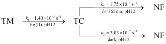
Scheme 1.
Kinetics constants for the TM decomposition through TC formation to non-fluorescent compound. TC consumption has been analyzed both in the presence of light (365 nm) and dark conditions.
4. Conclusions
Finally, the versatility and precision of the device are worth mentioning, as it provides data consistent with the literature. Specifically, it yields a value of 0.0021 s−1 for the first-order constant of TM oxidation when the excitation source is kept on for the strictly necessary time. However, if the excitation source remains on, this value significantly changes to 0.0014 s−1, which aligns with the value obtained in the consecutive mode process, where the excitation source is used similarly.
Additionally, the device’s versatility in sampling time is noteworthy, ranging from 10 ms, which allows for the determination of rate constants in the early stages, to measurements lasting several days, enabling the determination of rate constants six orders of magnitude lower. This feature is coupled with the ability to acquire a large number of wavelengths simultaneously.
Regarding potential improvements and device modifications, the usage of fiber optic elements and the incorporation of a stopped-flow system to achieve sampling limits of 10 ms are under consideration for the near future. Other fluorophores groups with potential activity in the near IR, which are involved in cancer imaging diagnostics, are currently under investigation.
Supplementary Materials
The following supporting information can be downloaded at: https://www.mdpi.com/article/10.3390/chemosensors13040128/s1, Text box S1. Speeding ‘analogRead’ SAM21D microcontroller original code. Text box S2. Speeding ‘analogRead’ SAM21D microcontroller proposed code. Table S1. Timing and statistics for different average options of ATSAM21DG18 AD converter. Figure S1. Excel screenshot capture debugging timer information. Figure S2. Schematics for the single array way storing trimmed spectra. Figure S3. Schematic for the relationship between sampling timing and the integration time. Figure S4. Stabilization of static measurements upon different pulse control methods to turn on the excitation light. Figure S5. Simplified flowchart: Initialization and Setup. Figure S6. LOOP subroutine flowchart. Figure S7. TC fluorescence emission spectra at different concentration levels for 365 nm excitation light. Figure S8. Logarithmic calibration plot for TC at 450 nm.
Author Contributions
Conceptualization: D.G.-A.; methodology: D.G.-A.; software and hardware: D.G.-A.; formal analysis: D.G.-A. and G.L.-P.; investigation: D.G.-A. and G.L.-P.; writing—original draft preparation: D.G.-A. and G.L.-P.; writing—review and editing: D.G.-A. and G.L.-P.; funding acquisition: G.L.-P. All authors have read and agreed to the published version of the manuscript.
Funding
This research has been partially supported by the Junta de Andalucía to the research group FQM-128, Universidad de Sevilla (VII Plan Propio de Investigación de la Universidad de Sevilla, 2024), and PID2021-126799NB-I00 funded by MCIN/AEI/ 10.13039/501100011033 and ERDF A way for making Europe, and European Union NextGenerationEU/PRTR.
Institutional Review Board Statement
Not applicable.
Informed Consent Statement
Not applicable.
Data Availability Statement
The data are contained within the article or Supplementary Materials.
Acknowledgments
The authors would especially like to thank Prof. Emilio Roldán González on the occasion of their retirement and Prof. Manuel M. Domínguez Pérez. We also wish to acknowledge B. Estepa Sánchez for providing the laboratory equipment and materials employed in this work.
Conflicts of Interest
The authors declare no conflict of interest.
References
- The Open Source Definition (Annotated). Available online: https://opensource.org/definition-annotated (accessed on 25 January 2025).
- Mehta, S.; Zhan, Y.; Roth, R.H.; Zhan, J.-F.; Mo, A.; Tenner, B.; Huganir, R.L.; Zhan, J. Single-fluorophore biosensors for sensitive and multiplexed detection of signaling activities. Nat. Cell. Biol. 2018, 20, 1215–1225. [Google Scholar] [CrossRef] [PubMed]
- Shi, Y.; Zhang, W.; Xue, Y.; Zhang, J. Fluorescent Sensors for Detecting and Imaging Metal Ions in Biological Systems: Recent Advances and Future Perspectives. Chemosensors 2023, 11, 226. [Google Scholar] [CrossRef]
- Nam, K.N. Fluorescent Protein-Based Metal Biosensors. Chemosensors 2023, 11, 216. [Google Scholar] [CrossRef]
- Hur, J.; Cho, J. Prediction of BOD, COD, and Total Nitrogen Concentrations in a Typical Urban River Using a Fluorescence Excitation-Emission Matrix with PARAFAC and UV Absorption Indices. Sensors 2012, 12, 972–986. [Google Scholar] [CrossRef]
- Wang, S.; Xu, J.; Yue, F.; Zhang, L.; Bi, N.; Gou, J.; Li, Y.; Huang, Y.; Zhao, T.; Jia, L. Smartphone-assisted mobile fluorescence sensor for self-calibrated detection of anthrax biomarker, Cu2+, and cysteine in food analysis. Food Chem. 2023, 451, 13410. [Google Scholar] [CrossRef]
- Wang, Z.; Yao, B.; Xiao, Y.; Tian, X.; Wang, Y. Fluorescent Quantum Dots and Its Composites for Highly Sensitive Detection of Heavy Metal Ions and Pesticide Residues: A Review. Chemosensors 2023, 11, 405. [Google Scholar] [CrossRef]
- Castro, R.C.; Páscoa, R.N.M.J.; Saraiva, M.L.; Lapa, R.A.S.; Fernandes, J.O.; Cunha, S.C.; Santos, J.L.M.; Ribeiro, D.S.M. Fluorometric kinetic determination of aflatoxin B1 by combining Cd-free ternary quantum dots induced photocatalysis and chemometrics. Microchem. J. 2023, 185, 108300–108311. [Google Scholar] [CrossRef]
- Skok, A.; Manousi, N.; Anthemidis, A.; Bazel, Y. Automated Systems with Fluorescence Detection for Metal Determination: A Review. Molecules 2024, 29, 5720. [Google Scholar] [CrossRef]
- Khan, J. Synthesis and Applications of Fluorescent Chemosensors: A Review. J. Fluoresc. 2024, 34, 2485–2494. [Google Scholar] [CrossRef]
- Pedras, B. (Ed.) Fluorescence in Industry from Springer Series on Fluorescence; Springer: Cham, Switzerland, 2019. [Google Scholar] [CrossRef]
- De Acha, N.; Elosúa, C.; Corres, J.M.; Arregui, F.J. Fluorescent Sensors for the Detection of Heavy Metal Ions in Aqueous Media. Sensors 2019, 19, 599. [Google Scholar] [CrossRef]
- Berden-Zrimec, M.; Drinovec, L.; Zrimec, A. Delayed Fluorescence. Chlorophyll a Fluorescence in Aquatic Sciences: Methods and Applications. In Developments in Applied Phycology; Suggett, D., Prášil, O., Borowitzka, M., Eds.; Springer: Dordrecht, The Netherlands, 2010; Volume 4. [Google Scholar] [CrossRef]
- Gu, Q.-S.; Li, T.; Yu, G.; Mao, G.-J.; Xu, F.; Li, C.-Y. Recent Advances in Design Strategies and Imaging Applications of Fluorescent Probes for ATP. Chemosensors 2023, 11, 417. [Google Scholar] [CrossRef]
- Wen-Li, J.; Wen-Xin, W.; Zhi-Qing, W.; Min, T.; Guo-Jiang, M.; Yongfei, L.; Chun-Yan, L. A tumor-targeting near-infrared fluorescent probe for real-time imaging ATP in cancer cells and mice. Anal. Chim. Acta 2022, 1206, 339798. [Google Scholar] [CrossRef]
- López-Pérez, G.; González-Arjona, D.; Roldán González, E.; Román-Hidalgo, C. Design of a Portable and Reliable Fluorimeter with High Sensitivity for Molecule Trace Analysis. Chemosensors 2023, 11, 389. [Google Scholar] [CrossRef]
- González-Arjona, D.; Roldán González, E.; López-Pérez, G.; Domínguez Pérez, M.M.; Calero-Castillo, M. Coulometer from a Digitally Controlled Galvanostat with Photometric Endpoint Detection. Sensors 2022, 22, 7541. [Google Scholar] [CrossRef]
- Microchip SAMD21 Datasheet. Available online: https://ww1.microchip.com/downloads/aemDocuments/documents/MCU32/ProductDocuments/DataSheets/SAM-D21-DA1-Family-Data-Sheet-DS40001882H.pdf (accessed on 25 January 2025).
- Hammatsu Mini-Spectrometer C12880MA Datasheet. Available online: https://www.hamamatsu.com/content/dam/hamamatsu-photonics/sites/documents/99_SALES_LIBRARY/ssd/miniature_spectrometer_kacc0012e.pdf (accessed on 25 January 2025).
- Parallax Data Acquisition Microcontroller Tool. Available online: https://www.parallax.com/package/plx-daq/ (accessed on 25 January 2025).
- PLX-DAQ. Version 2. Available online: https://forum.arduino.cc/t/plx-daq-version-2-now-with-64-bit-support-and-further-new-features/420628/71 (accessed on 25 January 2025).
- Cui, C.Q.; Qiu, L.L. Thiamine deficiency (beriberi) induced polyneuropathy and cardiomyopathy: Case report and review of the literature. J. Med. Cases. 2014, 5, 308–311. [Google Scholar] [CrossRef]
- Edwards, K.A.; Tu-Maung, N.; Cheng, K.; Wang, B.; Baeumner, A.J.; Kraft, C.E. Thiamine Assays-Advances, Challenges, and Caveats. ChemistryOpen 2017, 6, 178–191. [Google Scholar] [CrossRef]
- Conner, R.T.; Straub, G.J. Determination of Thiamin by the Thiochrome Reaction. Ind. Eng. Chem. 1941, 13, 380–384. [Google Scholar] [CrossRef]
- Holzbecher, J.; Ryan, D.E. The fluorimetric determination of phosphate with thiamine. Anal. Chim. Acta 1973, 64, 147–150. [Google Scholar] [CrossRef]
- Kusube, K.; Abe, K.; Hiroshima, O.; Ishiguro, Y.; Ishikawa, S.; Hoshida, H. Electrochemical Derivatization of Thiamine in Flow Injection System. Application to Thiamine Analysis. Chem. Pharm. Bull. 1983, 31, 3589–3594. [Google Scholar] [CrossRef][Green Version]
- Kusube, K.; Abe, K.; Hiroshima, O.; Ishiguro, Y.; Ishikawa, S.; Hoshida, H. Determination of Vitamin K Analogues by High Performance Liquid Chromatography with Electrochemical Derivatization. Chem. Pharm. Bull. 1984, 32, 179–184. [Google Scholar] [CrossRef]
- Ryan, M.A.; Miller, R.J.; Ingle, J.D., Jr. Intensified Diode Array Detector for Molecular Fluorescence and Chemiluminescence Measurements. Anal. Chem. 1978, 50, 1772–1777. [Google Scholar] [CrossRef]
- Ryan, M.A.; Ingle, J.D., Jr. Fluorometric Reaction Rate Method for the Determination of Thiamine. Anal. Chem. 1980, 52, 2177–2184. [Google Scholar] [CrossRef] [PubMed]
- Bower, N.W. Kinetic Fluorescence Experiment for the Determination of Thiamine. J. Chem. Edu. 1982, 59, 975–977. [Google Scholar] [CrossRef]
- Stepuro, I.I. Thiamine and vasculopathies. Prostaglandins. Leukot. Essent. Fatty. Acids. 2005, 72, 115–127. [Google Scholar] [CrossRef]
- Bubeshko, N.N.; Stsiapura, V.I.; Stepuro, I.I. Fluorescent Properties of Thiochrome in Solvents of Different Polarity. J. Appl. Spectrosc. 2011, 78, 337–343. [Google Scholar] [CrossRef]
- Speeding up Analogread() at the Arduino Zero. Available online: https://forum.arduino.cc/t/speeding-up-analogread-at-the-arduino-zero/426099/1 (accessed on 27 January 2025).
- Arduino Memory Guide. Available online: https://docs.arduino.cc/learn/programming/memory-guide (accessed on 26 January 2025).
- Miller, J.; Miller, J. Statistics and Chemometrics for Analytical Chemistry, 6th ed.; Prentice Hall: London, UK, 2010; ISBN 978-0-273-73042-2. [Google Scholar]
- Anwar, Z.; Sheraz, M.A.; Ahmed, S.; Mustaan, N.; Khurshid, A.; Gul, W.; Khattak, S.-U.-R.; Ahmad, I. Photolysis of Thiochrome in Aqueous Solution: A kinetic study. J. Photochem. Photobiol. B Biol. 2020, 203, 111766–111775. [Google Scholar] [CrossRef]
- Ahmad, I.; Abbas, S.H.; Anwar, Z.; Sheraz, M.A.; Ahmed, S.; Mobeen, M.F.; Mustaan, N.; Gul, W. Stability-Indicating Photochemical Method for the Assay of Thiamine by Spectrophotometry. J. Spectrosc. 2018, 2018, 3178518. [Google Scholar] [CrossRef]
- Define and Solve a Problem by Using Solver. Available online: https://support.microsoft.com/en-us/office/define-and-solve-a-problem-by-using-solver-5d1a388f-079d-43ac-a7eb-f63e45925040 (accessed on 26 January 2025).


Disclaimer/Publisher’s Note: The statements, opinions and data contained in all publications are solely those of the individual author(s) and contributor(s) and not of MDPI and/or the editor(s). MDPI and/or the editor(s) disclaim responsibility for any injury to people or property resulting from any ideas, methods, instructions or products referred to in the content. |
© 2025 by the authors. Licensee MDPI, Basel, Switzerland. This article is an open access article distributed under the terms and conditions of the Creative Commons Attribution (CC BY) license (https://creativecommons.org/licenses/by/4.0/).