Monitoring of Indoor Air Quality in a Classroom Combining a Low-Cost Sensor System and Machine Learning

Abstract

Monitoring indoor air quality in schools is essential, particularly as children are highly vulnerable to air pollution. This study evaluates the performance of the low-cost sensor-based air quality monitoring system ENSENSIA, during a 3-week campaign in an elementary school classroom in Athens, Greece. The system measured PM_2.5, CO, NO, NO₂, O₃, and CO₂. High-end instrumentation provided the reference concentrations. The aim was to assess the sensors’ performance in estimating the average day-to-day exposure, capturing temporal variations and the degree of agreement among different sensor units, with particular attention to the impact of machine learning (ML) calibration. Using the factory calibration settings, the CO₂ and PM_2.5 sensors showed strong inter-unit consistency for hourly averaged values. The other sensors, however, exhibited inter-unit variability, with differences in the reported average day-to-day concentrations ranging from 20% to 160%. ML-based calibration was investigated for the CO, NO, NO₂, and O₃ sensors using measurements by reference instruments for training and evaluation. Among the eleven ML algorithms tested, the Support Vector Regression performed better for the calibration of the CO, NO₂, and O₃ sensors. The NO sensor was better calibrated using the Elastic Net algorithm. The inter-unit variability was reduced by a factor of two after the ML calibration. The daily average error compared to the reference measured was also reduced by approximately 15–50% depending upon the sensor.

1. Introduction

Approximately 90% of the global population is exposed to polluted air [1] according to the World Health Organization (WHO), which leads to 7 million deaths annually [2,3,4]. Approximately 3.8 million of the deaths are attributed to indoor air pollution [5]. European citizens spend approximately 90% of their time indoors, primarily at home or in workplaces [1,2,6]. Indoor environments have additional sources of pollutants and can be more toxic than outdoor spaces [7]. Human exposure to harmful indoor air pollutants can be up to 100 times greater, in some cases, compared to outdoor air pollution [8,9,10].

The WHO has issued guidelines specifically addressing indoor air quality to protect public health from the risks associated with exposure to common indoor pollutants. These pollutants include particulate matter (PM_2.5 and PM₁₀), ozone (O₃), nitrogen dioxide (NO₂), sulfur dioxide (SO₂), and carbon monoxide (CO) [11], as well as benzene, formaldehyde, naphthalene, benzo[a]pyrene, radon, trichloroethylene, and tetrachloroethylene [12].

Children are vulnerable to the effects of air pollution [13,14] since they have higher breathing rates [15,16] and their organ systems are developing rapidly [16,17]. Moreover, children spend several hours every day in classrooms [16,18]. Increased CO₂ levels in classrooms indicate poor ventilation, which leads to reduced school attendance [19]. Long-term exposure to PM, NO₂, and SO₂ can impair lung development later in life [20]. Air pollution significantly impacts the central nervous system during childhood [21,22,23], potentially influencing behavior and academic performance [24].

Monitoring indoor air quality has traditionally relied on expensive, high-precision instruments with limited use in schools due to budget, size, and logistic constraints [1,25,26]. Recent advances in low-cost sensor technology offer a promising alternative, allowing for the more extensive monitoring of air quality in classrooms.

Low-cost sensors (LCSs) provide a viable solution to these challenges by offering an affordable and scalable means of monitoring air quality. These sensors include electrochemical sensors for gasses like NO and NO₂, laser-based sensors for PM, and nondispersive infrared sensors for CO₂, and are much cheaper than their high-precision counterparts. This cost advantage enables broader deployment across multiple classrooms and schools, facilitating air pollutant monitoring and timely interventions. Moreover, low-cost sensors are generally smaller and easier to install, requiring less specialized knowledge to operate and maintain. This makes them particularly suitable for environments in which resources and technical expertise may be limited. Due to their advantages, LCSs are increasingly used in air quality monitoring networks to provide real-time measurements with higher spatial density [5,27,28].

Despite these advantages, significant and unresolved issues surrounding LCSs still need to be addressed. These include questions about their performance capabilities for various uses and the lack of quality assurance tools. Generally, LCSs do not meet the performance standards set by regulatory equivalent reference instruments [5,29]. Also, LCSs often lack selectivity, meaning that sensors intended to measure carbon monoxide, for example, can be influenced by other pollutants—referred to as interfering gasses—that can skew the measured carbon monoxide values. This phenomenon is known as sensor cross-sensitivity [2]. Additionally, sensor lifetime and aging-related drifts can lead to a gradual degradation in performance over time, further impacting the reliability and accuracy of long-term measurements. In most cases, sensor lifetime typically varies from 3 to 6 years, after which performance may degrade significantly.

In their review of 40 studies of LCS usage, Saini et al. [10] stated that 31 studies (77.5%) did not report calibration procedure details, and accuracy was not specified in 39.4% of them. Only 22.5% of the studies reported field calibration or quality assurance methods. In another study, Chojer et al. [1] concluded that only 12 out of 35 studies using LCSs evaluated sensor performance. Thus, most practitioners still use such sensors, relying solely on factory calibration.

There has been a number of studies that have proposed calibration methods to improve the performance of LCS [30,31,32,33,34,35,36,37,38,39,40,41,42]. Although indoor air quality is affected by outdoor pollutants [43,44,45,46,47], calibration for the outdoor environment may not be sufficient for the indoor sensors. Sa et al. [34] reported that most studies evaluating LCS for indoor applications were conducted over short periods, with some lasting only a few minutes. Most studies focused on offices and homes, with kitchens and bedrooms being the most frequently studied rooms. Most (60%) studies focused on particulate matter, mainly in PM_2.5, followed by CO₂ (11 studies, 18%) and then CO (5 studies, 8%). Pollutants such as VOCs and ozone were less studied (four studies each, 6%), while only two studies evaluated NO₂ sensors (3%).

The present study evaluates a low-cost sensor-based air quality monitoring system, ENSENSIA [48,49], installed in a school in Athens, Greece. First, the variability between different sensors placed in the same classroom is assessed. Second, the performance of each low-cost sensor is quantified. This includes determining their accuracy and reliability in measuring PM_2.5, CO₂, CO, NO, and other relevant pollutants. By analyzing the data collected over three weeks, we investigate whether these sensors can reliably measure the average exposure of students to these pollutants on both a daily and hourly basis. Understanding this performance is crucial for determining whether these sensors can provide meaningful insights into the classroom’s air quality and help make informed decisions about interventions and improvements. Then, we evaluate the sensors’ ability to detect significant events that could impact air quality in the classroom, such as high emissions from traffic right outside the classroom. Finally, we evaluate several Machine Learning (ML) calibration models tailored to each type of sensor.

2. Materials and Methods

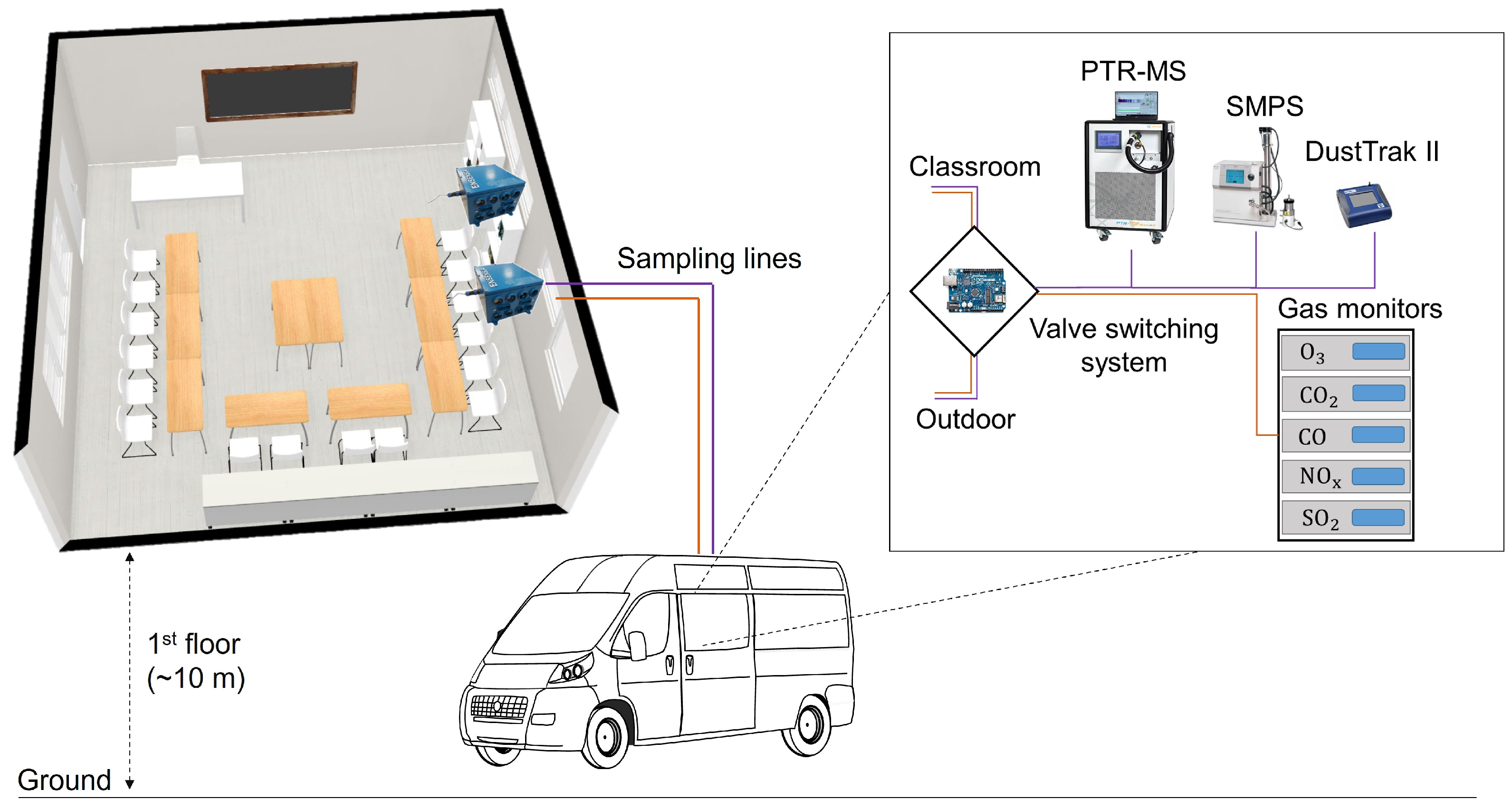
2.1. Measurement Site and Setup

Measurements were performed at the 8th primary school of Zografou, located close to the city center of Athens, a densely populated urban area. The school is located 5 km east of Athen’s center and is surrounded by residential buildings and a vehicle repair shop. The main road in front of the school is not part of a main artery; however, it has high traffic during early morning and early afternoon hours, as parents would drop off and pick up their children.

The investigated classroom is located in the school’s west wing on the first floor. Its windows face the school yard from the east side and residential homes and a vehicle repair shop from the west side. The classroom is 6.7 m (width), 6.8 m (length), and 2.9 m (height) and is used by 20 children and their teachers (Figure 1). The distance from the classroom to the next building on the west side is approximately 5 m and its distance from the yard is 2 m.

The FORTH mobile laboratory [50] was used to transport and house all the instrumentation (Figure 1). Five ENSENSIA systems (FORTH/ICE-HT, Patras, Greece) were installed, three outside of the school on the west side and two within the classroom. The reference instrumentation was inside the van. The particle size distribution was measured using a scanning mobility particle sizer (SMPS) (classifier model 3080, differential mobility analyzer (DMA) model 3081, condensation particle counter (CPC) model 3787, TSI, Shoreview, MN, USA), with a sheath flow rate of 5 L min⁻¹, a sample flow rate of 1 L min⁻¹, and a size range of 10 to 710 nm. Five gas phase monitors (Teledyne API, San Diego, CA, USA) were used to measure CO and CO₂ (Model 300E), O₃ (Model 400E), SO₂ (Model 100EU), and NO_x (Model T360).

The measurements started on 29 January (Monday) and lasted for three school weeks, until 16 February (Friday) of 2024. All reference instruments were used for both indoor and outdoor measurements. The instruments alternatively sampled indoor and outdoor air using a valve-switching system (Figure 1). Two sampling lines, a Teflon one for gasses and a copper one for particles [51], connected the classroom with the instruments in the FORTH mobile laboratory for indoor measurements. There were two additional sampling lines for the outdoor measurements. Changing between indoor and outdoor measurements was controlled by two automated switching three-way Swagelok valves, one for the gasses and one for the particles. The automated switching was controlled by a Pololu Maestro Servo Controller. During school hours, between 8:00 and 15:00, we sampled for 80 min indoors and then 20 min outdoors, while during non-school hours, we sampled for 20 min indoors and then 80 min outdoors.

We quantified the losses of pollutants in the sampling lines after the end of the experiments by sampling ambient air, both with a short sampling line and the long sampling line used in the classroom measurements. The average measured NO₂ with the short line was 11.5 ± 1.9 ppb and with the long line 11.2 ± 1.2 ppb. The difference of 0.3 ppb was not statistically significant. The same was observed for ozone. We measured 38.7 ± 1.9 ppb with the short line and 38.0 ± 1.1 ppb with the long line and the difference of 0.7 ppb was not statistically significant.

In contrast to the reference instrumentation, the five ENSENSIA systems were dedicated to indoor or outdoor measurements per their location (two inside the classroom and three outside of the classroom).

2.2. The ENSENSIA Sensor System

ENSENSIA is a multiple low-cost sensor system for monitoring outdoor and indoor air quality developed by FORTH/ICE-HT [48,49,52]. The system used in the present study contained six electrochemical sensors (CO, NO, NO₂, O₃, SO₂, and total VOCs), one nondispersive infrared CO₂ sensor, a laser sensor for measuring PM_2.5, and a sensor for measuring temperature and relative humidity. Detailed sensor ranges, models, units, and manufacturers are presented in

Table 1. Description of the low-cost sensors used in the ENSENSIA system.

Target Pollutant	Sensor Model	Range	Manufacturer
Ozone	OX-B431	0–200 ppb	Alphasense
Nitrogen Dioxide	NO2-B43F	0–200 ppb	Alphasense
Nitric Oxide	NO-B4	0–200 ppb	Alphasense
Carbon Monoxide	CO-B4	0–2000 ppb	Alphasense
Total VOCs	VOC-B4	0–10,000 ppb	Alphasense
Sulfur Dioxide	SO2-B4	0–200 ppb	Alphasense
Carbon Dioxide	COZIR-AH	0–10,000 ppm	Gas Sensing Solutions
Fine Particle Matter (PM2.5)	PMS5003	0–500 μg m−3	Plantower
Temperature	BME680	−40–85 °C	Bosch Sensortec
Relative Humidity	BME680	0–100%	Bosch Sensortec

.

2.3. Data Collection and Processing

2.3.1. Reference Data

The data from the high-end instrumentation were collected with either a 1 or 5 min averaging time. Upon collection, they were categorized into indoor and outdoor measurements. The first and last 5 min data points for each sample period were omitted from the analysis to avoid memory effects during the switching. Extreme outliers were also omitted from the dataset. The outliers were manually identified as sudden spikes in the time series, not attributed to an event, and were subsequently removed.

2.3.2. ENSENSIA Data

ENSENSIA uses a Raspberry PI (Model 4B) processing unit to gather the sensor output signals every 10 s. The module transmits averaged data every 2 min to a central server. Sensor data include the voltage output of the sensors’ electrodes, the pollutant concentrations according to the voltage-to-concentration equations provided by the sensors’ manufacturers, and environmental measurements (temperature and relative humidity).

The electrochemical sensors’ manufacturer (Alphasense Ltd., Essex, UK) provides equations to translate the electronic signal from each sensor to pollutant concentration values. These equations are different for each sensor, and they include the sensor’s working electrode (WE) electronic zero (WEe), auxiliary electrode (AE) electronic zero (AEe), WE zero (WE₀), AE zero (AE₀), and sensitivity (S).

The equations suggested by the electrochemical sensors’ manufacturer are as follows:

$$\mathrm{C}\mathrm{O}\left(\mathrm{p}\mathrm{p}\mathrm{b}\right)={\displaystyle \frac{\left(\mathrm{W}\mathrm{E}-\mathrm{W}\mathrm{E}\mathrm{e}\right)-\mathrm{n}\left(\mathrm{t}\right)\left(\mathrm{A}\mathrm{E}-\mathrm{A}\mathrm{E}\mathrm{e}\right)}{{\mathrm{S}}_{\mathrm{C}\mathrm{O}}}}$$

(1)

$$\mathrm{N}\mathrm{O}\left(\mathrm{p}\mathrm{p}\mathrm{b}\right)={\displaystyle \frac{\left(\mathrm{W}\mathrm{E}-\mathrm{W}\mathrm{E}\mathrm{e}\right)-\mathrm{k}(\mathrm{t})(\frac{{\mathrm{WE}}_0}{{\mathrm{AE}}_0})(\mathrm{A}\mathrm{E}-\mathrm{A}\mathrm{E}\mathrm{e})}{{\mathrm{S}}_{\mathrm{N}\mathrm{O}}}}$$

(2)

$${\mathrm{N}\mathrm{O}}_2\left(\mathrm{p}\mathrm{p}\mathrm{b}\right)={\displaystyle \frac{\left(\mathrm{W}\mathrm{E}-\mathrm{W}\mathrm{E}\mathrm{e}\right)-\mathrm{n}\left(\mathrm{t}\right)\left(\mathrm{A}\mathrm{E}-\mathrm{A}\mathrm{E}\mathrm{e}\right)}{{\mathrm{S}}_{{\mathrm{N}\mathrm{O}}_2}}}$$

(3)

$${\mathrm{O}}_3\left(\mathrm{p}\mathrm{p}\mathrm{b}\right)={\displaystyle \frac{\left(\mathrm{W}\mathrm{E}-{\mathrm{N}\mathrm{O}}_2-\mathrm{W}\mathrm{E}\mathrm{e}\right)-\mathrm{n}\left(\mathrm{t}\right)(\mathrm{A}\mathrm{E}-\mathrm{A}\mathrm{E}\mathrm{e})}{{\mathrm{S}}_{{\mathrm{O}}_3}}}$$

(4)

$${\mathrm{S}\mathrm{O}}_2\left(\mathrm{p}\mathrm{p}\mathrm{b}\right)={\displaystyle \frac{\left(\mathrm{W}\mathrm{E}-\mathrm{W}\mathrm{E}\mathrm{e}\right)-\mathrm{n}\left(\mathrm{t}\right)(\mathrm{A}\mathrm{E}-\mathrm{A}\mathrm{E}\mathrm{e})}{{\mathrm{S}}_{{\mathrm{S}\mathrm{O}}_2}}}$$

(5)

where parameters k and n are temperature-dependent and account for the influence of temperature on the signals.

For the PM_2.5 and CO₂ sensors, voltage-to-concentration conversion was performed using the default corrections provided by the manufacturers. The PM_2.5 sensor’s measurements were corrected using the methodology suggested by Kosmopoulos et al. [53].

Sensor data were averaged over 5 min, 15 min, and 60 min to facilitate comparative analysis using different time resolutions. During the sensor start-up phase, anomalous measurements may occur due to sensor stabilization. To address this, outliers during the start-up period were removed through manual inspection.

2.4. Sensor Calibration Using Machine Learning

The CO₂ sensor, using the factory calibration, showed acceptable performance and was excluded from the additional calibration process. PM_2.5 sensors’ measurements were directly compared to reference PM_2.5 and no further calibration was needed. We evaluated ML algorithms for calibrating the CO, NO, NO₂, and O₃ indoor ENSENSIA sensors.

The recent literature suggests that ML methods can account for sensor drifts, biases, and overall poor performance [35,48,54,55]. We developed several ML models and performed fine-tuning experiments to identify the optimal parameters and hyperparameters. These models included Extreme Gradient Boosting (XGBoost) [56], Random Forest (RF) [57], Categorical Boosting (CatBoost) [58], Light Gradient Boosting Machine (LightGBM) [59], K-Nearest Neighbors (KNN), Naïve Bayes (NB), Multiple Linear Regression (MLR), Support Vector Regression (SVR), Elastic Net, and Multilayer Perceptron (MLP) [60]. Brief algorithm descriptions are presented in the supplementary material.

ML models often perform better in the calibration of a specific sensor when they are allowed to consider the output signals of other sensors as well [49,61,62]. Therefore, to estimate the concentration of a specific pollutant (e.g., O₃), we supplied the responses of all available sensors as inputs to the ML models. The inputs provided to the models included the WE and AE voltages from the electrochemical sensors, concentrations of CO₂ and PM_2.5 from the corresponding sensors, temperature (T), and relative humidity (RH). These diverse inputs allowed the models to identify underlying relationships between sensor outputs and the target gas concentration. We implemented an exhaustive grid search method to iterate over every specific parameter combination to determine the optimal models’ parameters (Table S1). We used Python 3.9 and the libraries Pandas and Scikit Learn for such operations. Statistical calculations were made with the help of Scikit Learn and Statsmodels libraries.

Typically, an ML model requires training data to be built (training data) and a secondary dataset for validation (validation data). When additional external data are available, the ML model can be evaluated again on these data (external data or test data). Since the measurement campaign included only one school, external data were not included in this study.

To address this limitation and ensure the reliability of the models, we adopted a 5-fold cross-validation procedure. Τhe available data were divided into five equal parts or “folds”. The model was trained using data from four of the folds, while the remaining fold was used for validation. This process was repeated five times, with each fold being used once as the validation set. The model’s performance was then averaged across all five iterations, providing a more robust estimate of the accuracy and generalization capabilities.

To evaluate the effectiveness of the trained models in reducing discrepancies between identical sensors, we first trained the algorithm using data from one indoor sensor system. We then tested the trained model on a second indoor sensor system, which was positioned in close proximity to the first within the same classroom. This approach allowed us to assess the model’s ability to generalize and correct discrepancies across different but similar sensors.

2.5. Evaluation Metrics

The mean error (ME) and normalized ME (nME) or relative error are used to evaluate the low-cost sensor concentration values (P_i) against the actual values (O_i):

$$\mathrm{M}\mathrm{E}={\displaystyle \frac{\sum _{i=1}^n|P_i-O_i|}{n}}$$

(6)

$$\mathrm{n}\mathrm{M}\mathrm{E}={\displaystyle \frac{\sum _{i=1}^n|P_i-O_i|}{\sum _{i=1}^{n}Oi}}$$

(7)

In addition to these metrics, we employed the coefficient of determination (R²) to assess the goodness-of-fit of the model predictions. Furthermore, to evaluate the agreement between identical sensor units, we used the coefficient of divergence (COD) [63]. The COD in sensor time series data measures the dissimilarity between two sets of data collected by identical sensors over time. It provides insight into how much their patterns or behaviors differ and is given by the following equation:

$$\mathrm{C}\mathrm{O}\mathrm{D}=\sqrt{{\displaystyle \frac{{\sum }_{i=1}^N({\frac{P_i-O_i}{P_i+O_i})}^2}{N}}}$$

(8)

A COD value below 0.2 indicates a high degree of similarity between the two time series. The COD metric was used solely for comparing measurements between identical ENSENSIA sensors in the classroom and not for sensor evaluation against the reference instruments.

3. Results

3.1. Performance of Factory Calibration

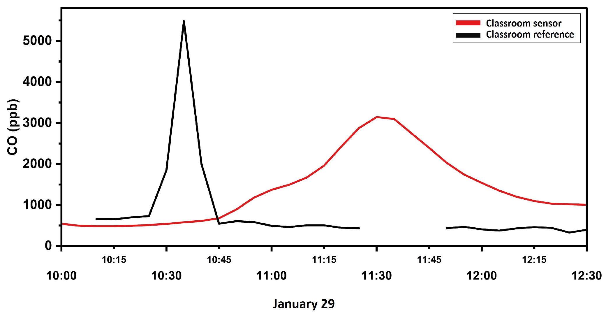
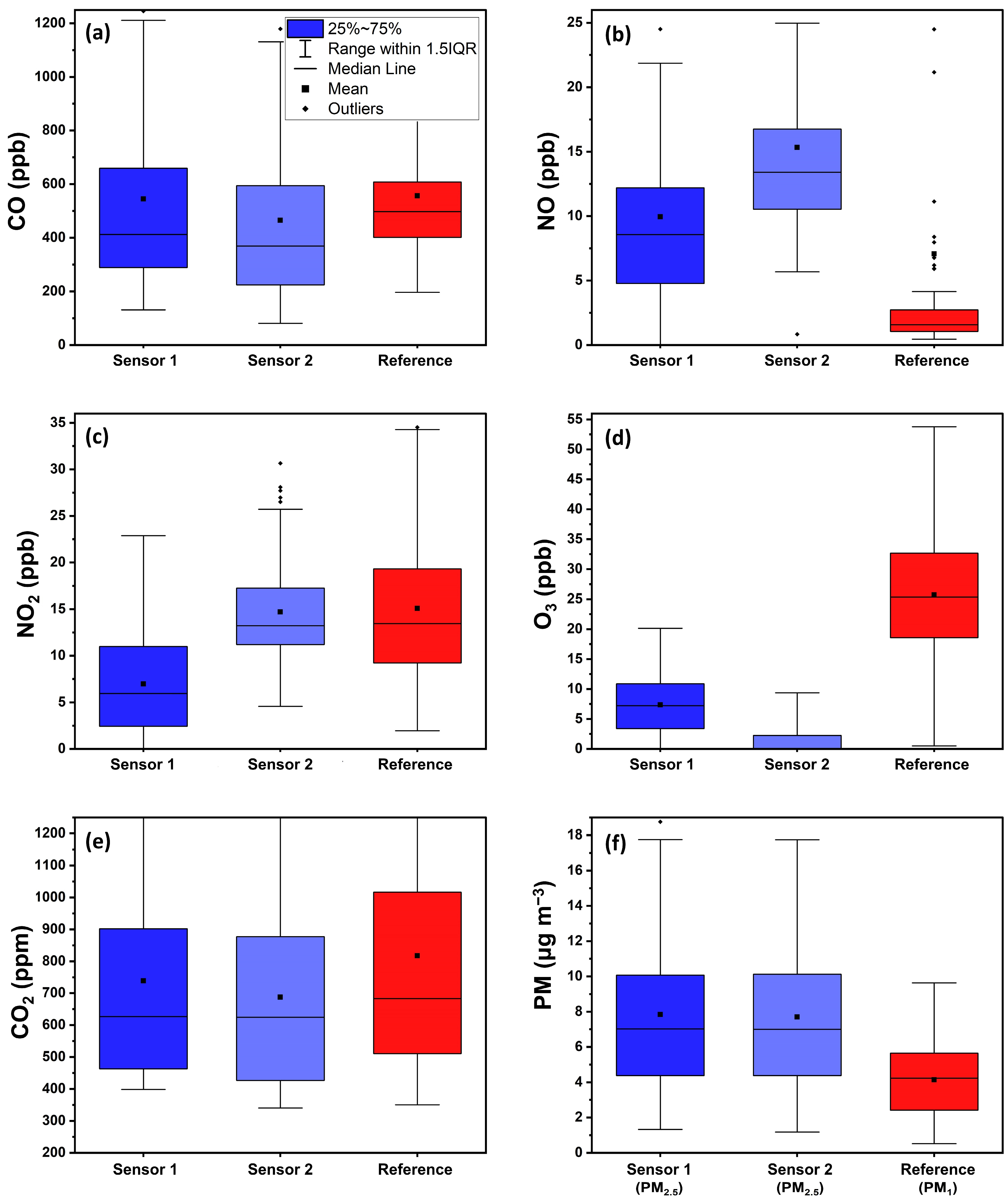
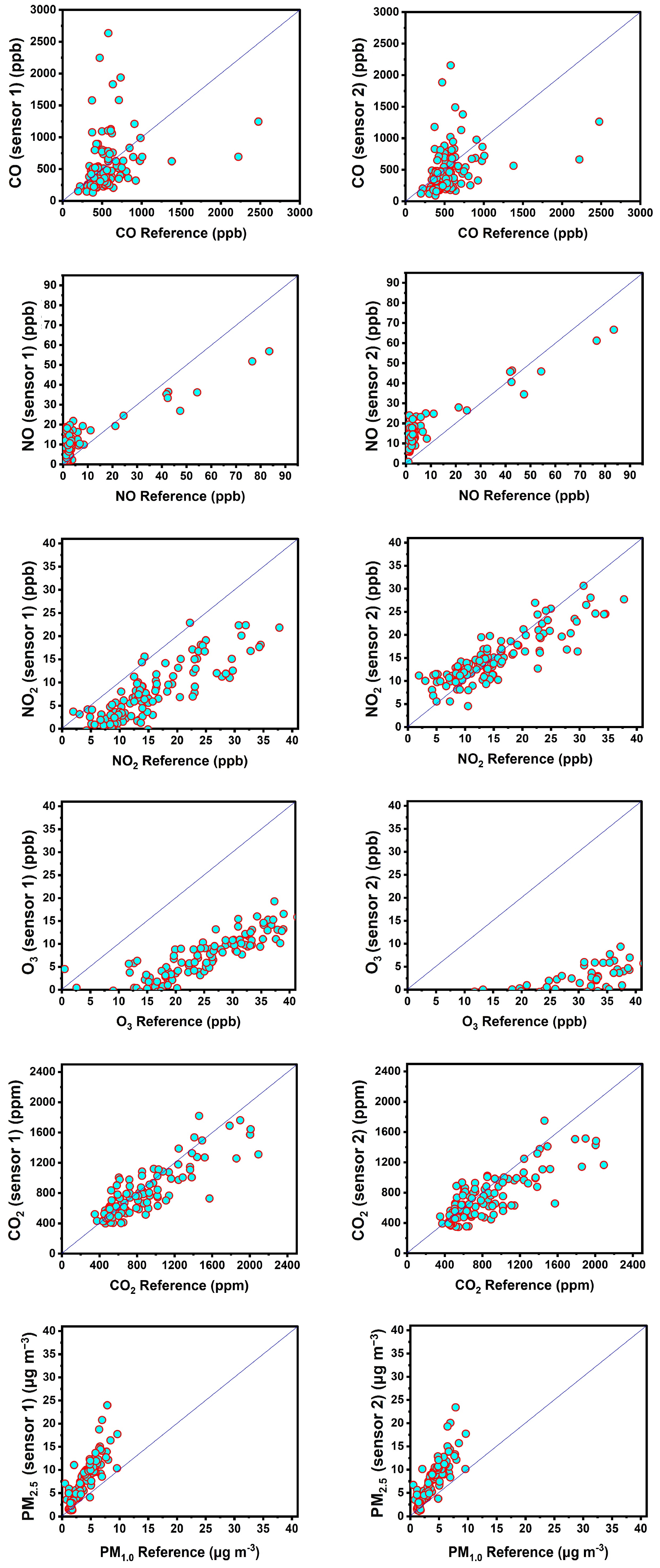
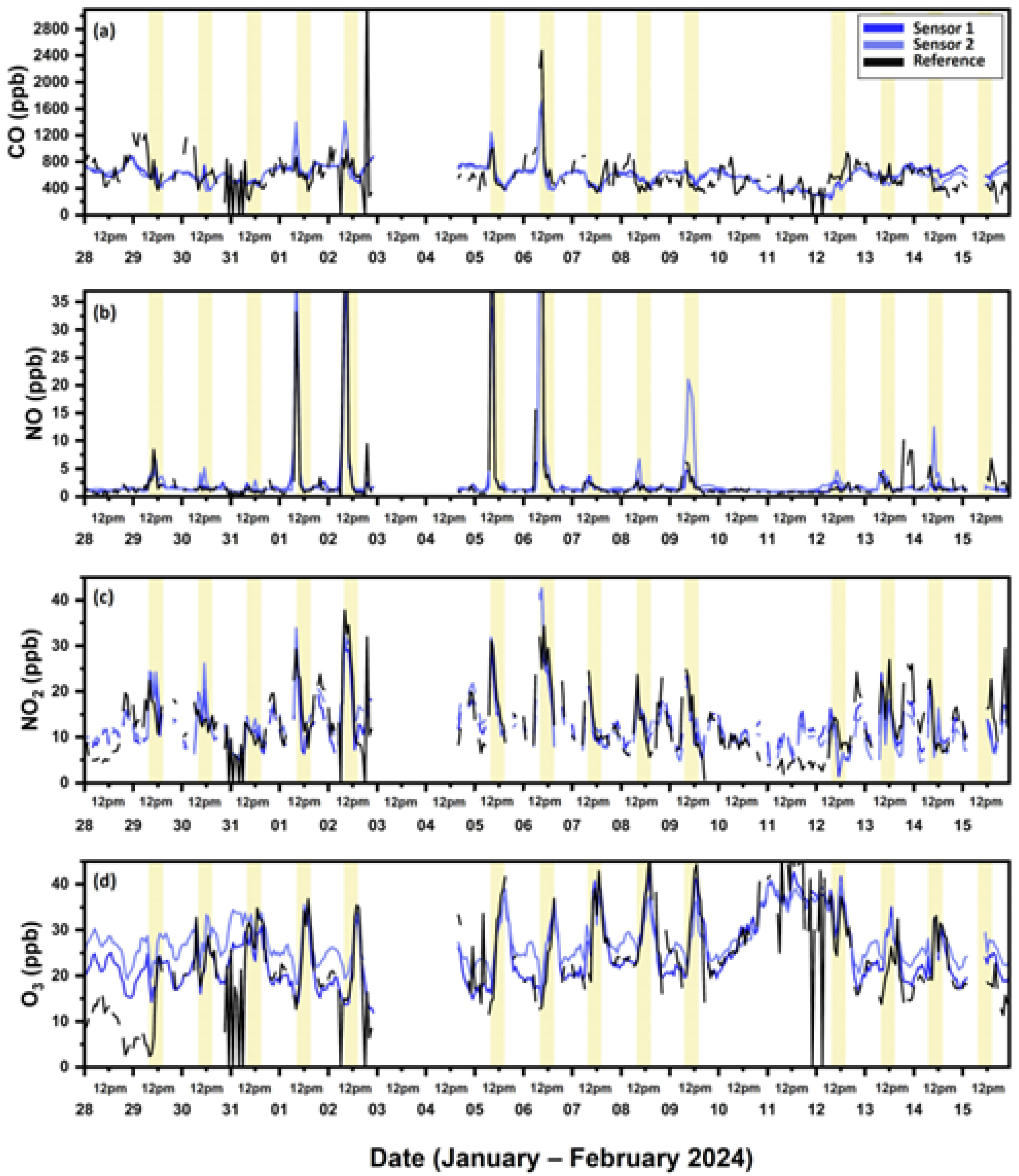
3.1.1. Carbon Monoxide

The hourly CO levels in the classroom during the campaign varied between 210 and 2000 ppb (554 ± 143 ppb) based on the reference measurements (Table S2). During February 6, CO in the classroom ranged between 400 and 1900 ppb (985 ± 570 ppb), higher than all the other days (Figure 2a). The gaps visible in Figure 2 correspond to the measurements taken outside the classroom, which were not included in this figure since it only shows the concentrations measured inside the classroom.

The two indoor CO sensors, at a 60 min averaging time, had an average discrepancy between them of 117 ppb (6%), an R² of 0.55, and a COD = 0.29 (

Table 2. Agreement between sensors in the classroom during school hours (08:00–14:00) using hourly averaged values. The average discrepancy is calculated using the same formula as the ME.

Sensor	Average Discrepancy	R2	COD
CO (Raw)	117 ppb	0.55	0.29
CO (Calibrated)	47 ppb	0.91	0.05
NO (Raw)	5 ppb	0.87	0.24
NO (Calibrated)	0.9 ppb	0.9	0.19
O3 (Raw)	7.7 ppb	0.7	0.32
O3 (Calibrated)	4 ppb	0.89	0.1
NO2 (Raw)	7 ppb	0.87	0.28
NO2 (Calibrated)	2.8 ppb	0.84	0.19
CO2 (Raw)	53 ppm	0.94	0.02
PM2.5 (Raw)	0.15 μg m−3	0.96	0.02
Total VOCs (Raw)	14 ppb	0.97	0.06

).

The daily (8 h averaging) exposure of the students to CO in the classroom was underestimated by 28% and 29% by the two indoor sensors, with MEs of 152 and 160 ppb, respectively (

Table 3. Performance metrics of the factory-calibrated indoor sensors during school hours (08:00–14:00) at multiple averaging times.

Sensor	5 min			15 min			60 min			8 h
	ME	nME	R2	ME	nME	R2	ME	nME	R2	ME	nME
CO	288, 263	51%, 47%	0.1, 0.13	290, 266	52%, 48%	0.1, 0.13	258, 238	48%, 44%	0.1, 0.15	152, 160	28%, 29%
NO	8.5, 12	139%, 197%	0.79, 0.85	8.3, 11.8	136%, 193%	0.78, 0.84	7.7, 11	126%, 180%	0.75, 0.84	5.3, 10	113%, 164%
NO2	8.9, 4.7	61%, 28%	0.65, 0.7	8.6, 3.5	61%, 30%	0.67, 0.72	8, 3.2	61%, 32%	0.7, 0.73	7.6, 2	58%, 21%
O3	18, 27	80%, 119%	0.75, 0.66	18, 26.5	80%, 115%	0.73, 0.61	18, 26	80%, 113%	0.75, 0.63	17, 25	72%, 110%
CO2	150, 145	18%, 17%	0.72, 0.73	160, 145	20%, 17%	0.64, 0.71	136, 124	17%, 15%	0.72, 0.74	92, 81	11%, 9%
PM2.5	-	-	0.77, 0.7	-	-	0.72	-	-	0.70	-	-

CO, NO, NO₂, and O₃ sensor’s and reference’s measurements are in ppb. CO₂ measurements are in ppm. PM_2.5 measurements are in μg m⁻³.

, Figure 2), when compared to the reference instrument. The R² of the indoor sensors for these daily averages was 0.1 and 0.15, respectively (Table 3).

Multiple averaging times (5 min, 15 min, 60 min) produced similar errors for indoor sensors compared to reference measurements during school hours, with the 60 min averaging being marginally better (Table 3). Specifically, at 60 min averaging, the first CO sensor had a ME of 258 ppb (49%) and the second CO sensor 238 ppb (44%). The temporal variation of the concentration was not followed by any of the sensors (R² = 0.1), even for the 60 min averaging interval (Table 3).

Examining the performance of the two indoor CO sensors at 60 min averaging from day to day, the nME for each day varied widely, ranging between 16% and 124% (Table S2, Figure S1). The sensors’ performance demonstrated variability over the monitoring period, with periods of both high and low accuracy (Figure 2). On the day when the 8 h-averaged reference CO concentration was notably elevated (1000 ppb), the sensors exhibited a nME of 63%. This value falls within the intermediate range between the lowest and highest recorded errors during the campaign. A similar pattern is observed when analyzing the temporal trend over multiple days at 60 min averaging, as reflected in the R² value, which ranged from 0.02 to 0.86 (Table S2, Figure S2a).

On 29 January, at 10:30, the mobile laboratory (van) was started (cold start), and the indoor CO concentration increased to 5500 ppb according to the reference instrument. The low-cost sensor did not respond to this 5–10 min elevated concentration (Figure 3).

Despite the sensor’s limitations in capturing the temporal indoor CO variation even at 60 min averaging, the CO sensors are capable of estimating the average daily student exposure (8 h averaging) to CO with approximately 29% nME.

3.1.2. Nitric Oxide

The hourly NO levels in the classroom during school hours ranged from 0.6 to 83 ppb (6 ± 7 ppb) based on the reference instrument (Table S3). While both classroom NO sensors had the same trend (R² = 0.87), the NO concentration measured by the second sensor was systematically shifted by 5 ppb (Figure 4). This offset suggests a factory calibration discrepancy or inherent bias in the second sensor. This problem is also reflected in the COD metric (0.24).

During school hours, the indoor sensors had hourly ME of 7.7 and 11 ppb, R² of 0.75 and 0.84, and nME of 26% and 80%, respectively (Table 3), compared to the reference instrument. Both sensors persistently overestimated the actual concentration (Figure 5). At 5 min and 15 min averaging times, the sensors performed marginally worse than at 60 min in terms of ME and nME (Table 3).

During the four days that the average reference NO concentration during school hours was elevated (>12 ppb, Figure 5 and Figure S1), the sensor average error was significantly lower than the other days (ME 1.5 pbb, nME 8%).

3.1.3. Nitrogen Dioxide

Based on the reference measurements, indoor and outdoor hourly NO₂ concentrations were similar and consistent during the campaign. Indoor NO₂ varied between 5.6 and 38 ppb (16 ± 5 ppb) and outdoor between 6 and 40 ppb (16 ± 5 ppb).

The two indoor sensors showed a similar trend (R² = 0.87) at 60 min averaging, but the second sensor measured 50% lower values than the first (Figure 4), resulting in an average hourly discrepancy of 7 ppb (95%).

Using 8 h averaged data (08:00–16.00), the two sensors had a ME of 7.6 ppb (58%) and 2 ppb (21%) when compared to the reference concentrations. The first sensor persistently underestimated the actual NO₂ concentrations in the classroom and the second sensor underestimated concentrations above 20 ppb (Figure 5).

Averaging the sensors data by 5 min, 15 min, and 60 min had a minimal effect on their performance (Table 3). At hourly averages and only during school hours, the first sensor had an ME of 8 ppb (61%) and the second one 3.2 ppb (32%). The R² values (between the sensors and the reference instrument) were 0.75 and 0.84, respectively (Table S4).

The sensors detected all NO₂ peaks (>25 ppb) during school hours (Figure 5), consistent with the reference measurements. They also showed increased NO₂ concentrations during days when the actual NO₂ was elevated (2, 5, and 6 February 2024, Table S4).

3.1.4. Ozone

Hourly O₃ concentrations in the classroom during school hours based on the reference measurements varied from close to zero to 46 ppb. The average concentration during all school hours was approximately 30 ppb (Table S5). Ambient O₃ was persistently higher (about 10–15 ppb) outside than inside the classroom.

The hourly averaged readings of the two indoor sensors had a significant discrepancy of 7.7 ppb (Table 2) with each other, and their corresponding COD value was 0.32. The two sensors had similar temporal patterns (R² = 0.7) at 60 min averaging.

Using 8 h averaged data (08:00–16.00), the first sensor exhibited a ME of 17 ppb (72%) and the second 25 ppb (110%) when compared to the reference instrument. Both sensors underestimated the actual concentrations (Figure 4 and Figure 5).

At hourly resolution, the sensors’ MEs was 18 ppb (80%) and 26 ppb (113%), respectively (Table 3). The sensors had similar performance for the three averaging periods.

Both indoor sensors captured the O₃ trends over time with hourly averaged R² values of 0.75 and 0.63, respectively (Table S5, Figure S2). O₃ generally peaked in the classroom after 12:00 LT (Figure 4d), and the sensors also followed this behavior, but measured approximately half of the actual concentration.

3.1.5. Carbon Dioxide

CO₂ was elevated during school hours, as expected. The hourly average concentration was around 700 ppm with a standard deviation of 300 ppm (Table S6). The minimum hourly recorded concentration during schooltime was 420 ppm and the maximum was close to 3000 ppm.

The two indoor sensors had a mean hourly discrepancy with each other of 53 ppm and an R² of 0.94 (Table 2). The COD was 0.02. Using 8 h averaging (08:00–16.00), the recorded ME of the first sensor was 92 ppm (nME of 11%) and of the second sensor 81 ppm (nME of 9%) compared to the reference instrument. The sensors’ performance at multiple averaging times was similar (Table 3). At hourly resolution, the first sensor exhibited a ME of 136 ppm (nME = 17%) and the second one 124 ppm (nME = 15%) compared to the reference instrument. The sensors showed consistent performance across the various days (Figures S1 and S2).

The sensors captured the increased indoor CO₂ during the school days and hours (Figure 5). However, the sensors’ R² (compared to the reference concentration) at 60 min averaging varied from day to day, ranging from 0.24 to 0.96. The R² value was above 0.74 for most of the days (Table S6).

3.1.6. Fine Particle Matter

The reference PM₁ concentrations at hourly resolution varied between 1 and 8 μg m⁻³. The maximum observed value at the same time resolution was 11 μg m⁻³ (Table S7).

The two PM_2.5 sensors had an almost perfect agreement with each other (average discrepancy 0.15 μg m⁻³, Table 2) and an almost perfect R² of 0.96. The sensor values correlated with the reference instrument at all averaging periods (R² = 0.7 at 60 min, Table S1). Also, the two sensors persistently read PM_2.5 values higher than the actual PM₁ concentration by 3.8 μg m⁻³ on average (Table S7).

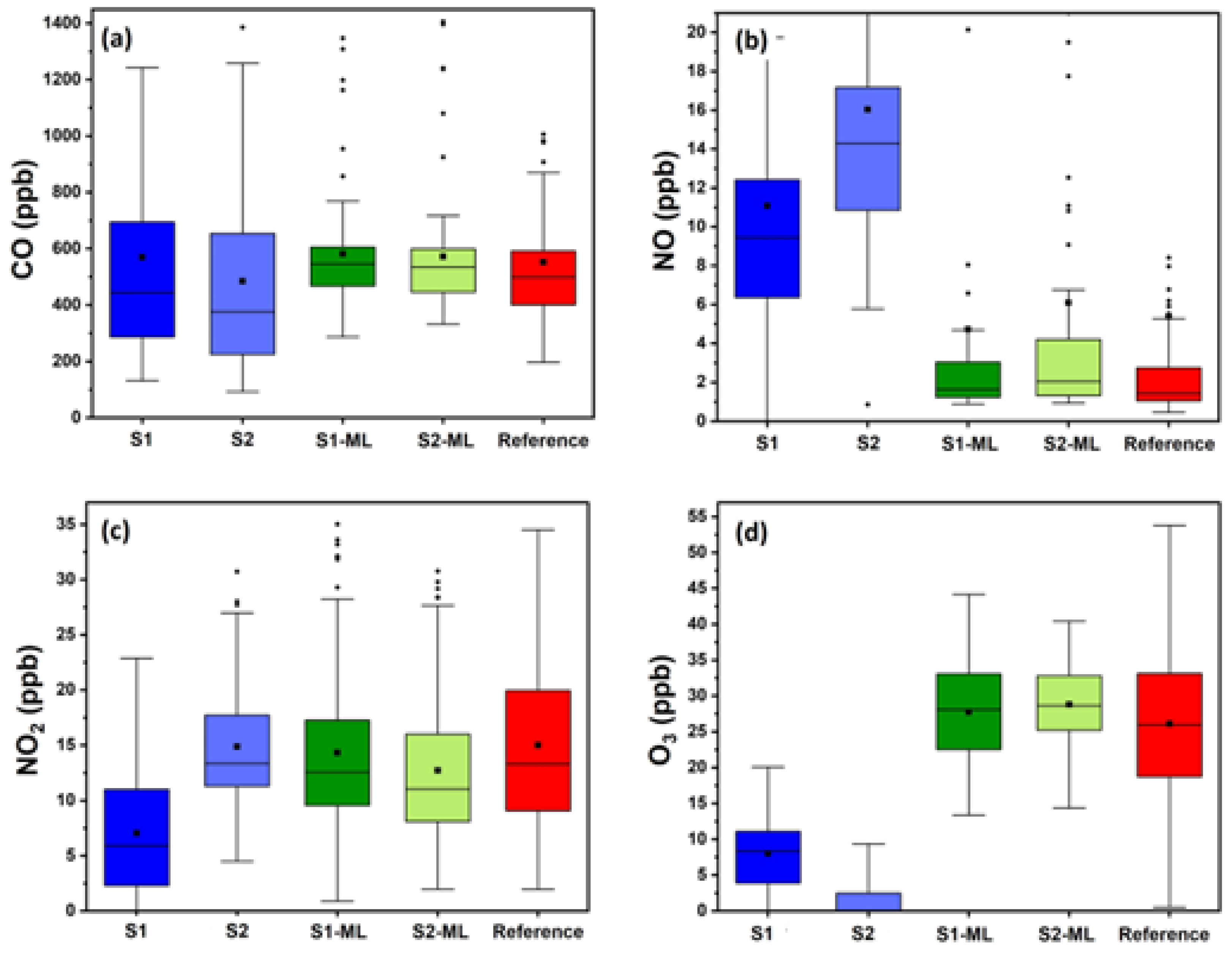
3.2. Performance of ML Calibration

The performance of ML-based calibration models varied depending on the sensor. SVR was the optimal model for the CO, NO₂, and O₃ sensors and Elastic Net for the NO sensor. Tables S8–S11 summarize the evaluation metrics at hourly averaging for all ML calibration approaches.

After calibrating the two indoor CO sensors with SVR, their 8 h average ME decreased from 152 ppb (sensor 1) and 238 ppb (sensor 2) to 135 ppb (1% and 43% reduction, respectively). The resulting nME was 23%. The sensors also performed well on days with higher CO concentrations (Figure 6). Using 60 min averaging, the ME was reduced for both sensors to 193 and 201 ppb, respectively (

Table 4. ML-calibration performance metrics of the indoor sensors during school hours (08:00–14:00) at multiple averaging times.

Sensor	5 min			60 min			Average Day-to-Day (8 h)
	ME	nME	R2	ME	nME	R2	ME	nME	R2
CO	193, 201	35%, 33%	0.16	138, 141	25 %	0.25, 0.22	135	23%	-
NO	3.4, 4.2	56%, 65%	0.72, 0.83	3, 3.5	49%, 57%	0.9, 0.87	2, 3	33%, 49%	-
NO2	4	33%	0.6	3.2, 3.4	30%, 34	0.71, 0.69	3	30%	-
O3	4, 5.5	15%, 21%	0.66, 0.65	4, 5.5	15%, 21%	0.75, 0.63	4, 5	16%, 19%	-

CO, NO, and O3 sensor’s measurements are in ppb.

). The latter equals a reduction of 33%. The R² increased from near zero to 0.25 and 0.22 for the two sensors. Finally, the R² showed significant variability from day to day (lowest = 0.1 and highest = 0.99). Overall, the sensor’s response was significantly improved with ML calibration at hourly resolution, but the temporal variations in CO concentrations during specific days were not captured (Table S12, Figure 6).

Calibration using Elastic Net had a significant impact on the NO sensor’s results. At 8 h averaging, the nME of the two calibrated indoor sensors was reduced from 113% to 33% and from 164% to 49%, respectively. The hourly ME of the two sensors was reduced from 7.7 to 3 ppb (39% reduction) and from 11.8 to 3.5 ppb (70% reduction) after calibration. The R² increased from 0.75 to 0.9 and from 0.84 to 0.87, respectively (Table 4). During days with elevated NO concentrations, the sensor’s errors were significantly lower (Table S13). For example, on February 2, the 1 h average reference NO concentration was 16 ± 21 ppb, and the calibrated sensor read 15 ± 19 ppb, resulting in an nME of 18% and an R² of 0.99. Similar behavior was observed during the rest of the days (Figure 6, Figure 7 and Figure 8).

The calibration of the two indoor NO₂ sensors with SVR reduced the 8 h average ME from 7.6 ppb (58%) and 3.2 ppb (32%) to 3 ppb (30%). The performance of the calibrated sensors was consistent throughout the campaign days (Table S14, Figure 6). For hourly averaged values, the ME was reduced from 8.6 ppb (61% nME) and 3.5 ppb (34% nME) to 3.2 ppb (30%) and 3.4 ppb (34% nME). R² at 60 min averaging was also slightly improved for one of the two sensors, from 0.67 to 0.71. For the other sensor, it was reduced from 0.72 to 0.69. Like the NO sensor, the NO₂ sensor showed lower absolute and relative errors on days with higher observed NO₂ concentration. For example, on February 6, the actual hourly averaged concentration was 27 ± 5 ppb, whilst the calibrated sensors read 28 ± 9 ppb (ME = 6.8 ppb, nME = 28%). Temporal NO₂ at 60 min averaging were captured by the sensor (Figure 6).

For the O₃ sensors, calibration using SVR reduced the 8 h average ME from 17 ppb (72% nME) and 26 ppb (110% nME) to 4 ppb (16% nME) and 5 pbb (19% nME). The performance of the calibrated sensors was consistent throughout the campaign days (Table S15, Figure 6 and Figure S4). For hourly averaged values, the ME of the two sensors was reduced from 18 ppb (80% nME) and 26.5 ppb (115% nME) to 4 ppb (15% nME) and 5.5 ppb (21% nME). At the same time resolution, R² remained at 0.75 for the first sensor and improved from 0.61 to 0.63 for the second.

3.3. Impact of ML on Inter-Unit Consistency

Table 2 shows the average discrepancy (ME), R², and COD of the indoor sensors using hourly averaged values. These metrics were selected as the most representative metrics for assessing inter-unit consistency.

Calibrating the CO sensors with ML improved the R² and COD between them (R² increased to 0.91 from 0.55 and COD was reduced to 0.05 from 0.29) and significantly reduced the average discrepancy (from 117 to 47 ppb) for the hourly averaged values.

For the NO sensor, ML calibration reduced the discrepancy between sensors from 5 ppb to 0.9 ppb and increased the R² from 0.87 to 0.9 at hourly resolution. The COD also decreased to 0.19 from 0.24. The Elastic Net model maintained the already high R² and reduced the systematic offset among the two sensors.

Calibration with SVR improved the agreement between the NO₂ sensors, reducing the hourly average discrepancy from 7 ppb to 2.8 ppb. The COD value declined to 0.19 from 0.28 and R² remained at 0.87.

Finally, SVR calibration improved the agreement between the O₃ sensors. The hourly average discrepancy declined to 4 ppb from 7.7 ppb. Similar improvements were observed in the R² and COD metrics (R² reached 0.89 from 0.7 and COD decreased to 0.1 from 0.32).

4. Discussion and Conclusions

The factory-calibrated CO₂ sensors in the classroom agreed with each other (average discrepancy of 53 ppb, nME 8%, R² at 0.94 at hourly averages). Similarly, the factory-calibrated PM_2.5 sensors strongly agreed with each other (average discrepancy of 0.15 μg m⁻³, nME 2%, R² at 0.96 at hourly averages). However, the CO, NO, O₃, and NO₂ sensors exhibited significant inter-unit variability (>60%) using their factory calibration.

The average performance of the factory-calibrated sensors during school hours was assessed by averaging their measurements over an 8 h period (08:00–16:00) and comparing them against the reference measurements. The factory-calibrated indoor CO₂ sensors exhibited the best performance, with a relative error of 9% and 11% (81 and 92 ppm), respectively. The factory-calibrated CO sensors had relative errors of 28% and 29% (152 and 160 ppb), respectively. For the NO sensors, the corresponding relative errors were 113% and 164% (5.3 and 10 ppb). The NO₂ sensors had relative errors 58% and 21% (7.6 and 2 ppb), whilst the O₃ sensors had 72% and 110% (17 and 25 ppb). The performance of all sensors was consistent during the campaign days.

We also used 15 min averaging for assessing the sensors’ temporal performance during a class. The CO₂ sensors captured concentration fluctuations during school hours (R² > 0.7), when occupancy levels rose and led to elevated CO₂ concentrations. The factory-calibrated NO₂ sensors also captured temporal changes in indoor concentrations (R² ranged between 0.67 and 0.72). Similar behavior was observed for the PM_2.5 (R² = 0.72) and O₃ sensors (R² ranging between 0.61 and 0.73). The NO sensor showed inconsistent R² values from day to day, ranging from 0.1 to 0.96. Finally, the CO sensors were not able to capture either concentration changes happening within 15 min or hourly (the R² of both sensors for 5 min and 60 min averages remained below 0.1).

The optimal ML calibration method for the CO, NO₂, and O₃ sensors was SVR and, for the NO sensor, Elastic Net. Calibration using ML models significantly improved the inter-unit consistency of these sensors. The hourly average discrepancy between the CO, NO, NO₂, and O₃ sensors was decreased by 60, 98, 48, and 60%, respectively. The resulting hourly discrepancy was 47 ppb for the CO sensors, 1 ppb for the NO sensors, 2.8 ppb for the NO₂ sensors, and 4 ppb for the O₃ sensors. All post-calibration COD values were below 0.05, except for the NO and NO₂ sensors (COD = 0.19). All R² values increased above 0.84 post-calibration. Due to absence of adequate training data for reference NO concentrations above 50 ppb, an evaluation of the factory- and ML-calibrated sensors’ response was prohibited.

ML calibration significantly improved the accuracy of the CO, NO, NO₂, and O₃ sensors in estimating the average day-to-day student exposure (during school hours). The relative errors (nME) of the CO sensors were reduced to 23%, the NO₂ sensors to 30%, the O₃ sensors to 16 and 19%, and the NO sensors to 33% and 49%. The ML-calibrated sensors’ performance was similar from day to day. The 8 h ME of the calibrated CO, O₃, NO₂, and NO sensors were 135 ppb, 4.5 ppb, 3 ppb, and 2.5 ppb. Slight improvements in the hourly averaged R² values were also observed post-calibration for the NO, NO₂, and O₃ sensors.

The approach of training the ML models using data from the first sensor system and evaluating them on the second sensor system within the same environment represents an important initial step toward developing a generalized calibration model for future sensor deployments in classrooms. The results of the present study demonstrate that the trained ML algorithms can effectively mitigate discrepancies between identical sensors under similar conditions whilst improving their overall agreement with the reference instruments. However, when the trained model is exposed to entirely different conditions in various classrooms, its effectiveness is not guaranteed. The short duration of the present study (3 weeks) and the absence of external test sets decreases the adaptability of the ML models. Further research is necessary to evaluate the models’ transferability across various classrooms and to determine whether additional fine-tuning or domain adaptation techniques are required. A limitation of this study is the lack of a stabilization period for the electrochemical sensors before deployment. Baseline offsets may occur without sufficient time to adapt to the specific conditions. In this case, sensors were not stabilized in situ for the recommended 1–3 weeks, which could have contributed to measurement inaccuracies.

Finally, the total VOC sensor and SO₂ sensor are currently subject to evaluation and the corresponding results will be discussed in a future publication.

References

1. Chojer, H.; Branco, P.T.B.S.; Martins, F.G.; Alvim-Ferraz, M.C.M.; Sousa, S.I.V. Development of Low-Cost Indoor Air Quality Monitoring Devices: Recent Advancements. Sci. Total Environ. 2020, 727, 138385. [Google Scholar] [CrossRef] [PubMed]
2. Suriano, D.; Penza, M. Assessment of the Performance of a Low-Cost Air Quality Monitor in an Indoor Environment through Different Calibration Models. Atmosphere 2022, 13, 567. [Google Scholar] [CrossRef]
3. World Health Organization Ambient (Outdoor) Air Pollution. Available online: https://www.who.int/news-room/fact-sheets/detail/ambient-(outdoor)-air-quality-and-health (accessed on 9 September 2024).
4. World Health Organization How Air Pollution Is Destroying Our Health. Available online: https://www.who.int/news-room/spotlight/how-air-pollution-is-destroying-our-health (accessed on 9 September 2024).
5. Ródenas García, M.; Spinazzé, A.; Branco, P.T.B.S.; Borghi, F.; Villena, G.; Cattaneo, A.; Di Gilio, A.; Mihucz, V.G.; Gómez Álvarez, E.; Lopes, S.I.; et al. Review of Low-Cost Sensors for Indoor Air Quality: Features and Applications. Appl. Spectrosc. Rev. 2022, 57, 747–779. [Google Scholar] [CrossRef]
6. European Commission Indoor Air Pollution: New EU Research Reveals Higher Risks than Previously Thought. 22 September 2003. Available online: https://ec.europa.eu/commission/presscorner/detail/en/ip_03_1278 (accessed on 9 September 2024).
7. EPA The Inside Story: A Guide to Indoor Air Quality. Available online: https://www.epa.gov/indoor-air-quality-iaq/inside-story-guide-indoor-air-quality (accessed on 9 September 2024).
8. Anand, P.; Sekhar, C.; Cheong, D.; Santamouris, M.; Kondepudi, S. Occupancy-Based Zone-Level VAV System Control Implications on Thermal Comfort, Ventilation, Indoor Air Quality and Building Energy Efficiency. Energy Build. 2019, 204, 109473. [Google Scholar] [CrossRef]
9. Cincinelli, A.; Martellini, T. Indoor Air Quality and Health. Int. J. Environ. Res. Public Health 2017, 14, 1286. [Google Scholar] [CrossRef]
10. Saini, J.; Dutta, M.; Marques, G. Sensors for Indoor Air Quality Monitoring and Assessment through Internet of Things: A Systematic Review. Environ. Monit. Assess. 2021, 193, 66. [Google Scholar] [CrossRef] [PubMed]
11. World Health Organization. WHO Global Air Quality Guidelines: Particulate Matter (PM2.5 and PM10), Ozone, Nitrogen Dioxide, Sulfur Dioxide and Carbon Monoxide, xxi, ed.; World Health Organization: Geneva, Switzerland, 2021; ISBN 978-92-4-003422-8. [Google Scholar]
12. World Health Organization. Who Guidelines for Indoor Air Quality: Selected PollutantsWHO: Copenhagen, Denmark, 2010; ISBN 978-92-890-0213-4.
13. Arcega-Cabrera, F.; Fargher, L.; Quesadas-Rojas, M.; Moo-Puc, R.; Oceguera-Vargas, I.; Noreña-Barroso, E.; Yáñez-Estrada, L.; Alvarado, J.; González, L.; Pérez-Herrera, N.; et al. Environmental Exposure of Children to Toxic Trace Elements (Hg, Cr, As) in an Urban Area of Yucatan, Mexico: Water, Blood, and Urine Levels. Bull. Environ. Contam. Toxicol. 2018, 100, 620–626. [Google Scholar] [CrossRef]
14. Iglesias-González, A.; Hardy, E.M.; Appenzeller, B.M.R. Cumulative Exposure to Organic Pollutants of French Children Assessed by Hair Analysis. Environ. Int. 2020, 134, 105332. [Google Scholar] [CrossRef]
15. Landrigan, P.J.; Fuller, R.; Acosta, N.J.R.; Adeyi, O.; Arnold, R.; Basu, N.; Baldé, A.B.; Bertollini, R.; Bose-O’Reilly, S.; Boufford, J.I.; et al. The Lancet Commission on Pollution and Health. Lancet 2018, 391, 462–512. [Google Scholar] [CrossRef]
16. Zhu, Y.; Li, X.; Fan, L.; Li, L.; Wang, J.; Yang, W.; Wang, L.; Yao, X.; Wang, X. Indoor Air Quality in the Primary School of China—Results from CIEHS 2018 Study. Environ. Pollut. 2021, 291, 118094. [Google Scholar] [CrossRef]
17. Hoek, G.; Pattenden, S.; Willers, S.; Antova, T.; Fabianova, E.; Braun-Fahrländer, C.; Forastiere, F.; Gehring, U.; Luttmann-Gibson, H.; Grize, L.; et al. PM 10, and Children’s Respiratory Symptoms and Lung Function in the PATY Study. Eur. Respir. J. 2012, 40, 538–547. [Google Scholar] [CrossRef] [PubMed]
18. Pacitto, A.; Amato, F.; Moreno, T.; Pandolfi, M.; Fonseca, A.; Mazaheri, M.; Stabile, L.; Buonanno, G.; Querol, X. Effect of Ventilation Strategies and Air Purifiers on the Children’s Exposure to Airborne Particles and Gaseous Pollutants in School Gyms. Sci. Total Environ. 2020, 712, 135673. [Google Scholar] [CrossRef] [PubMed]
19. Gaihre, S.; Semple, S.; Miller, J.; Fielding, S.; Turner, S. Classroom Carbon Dioxide Concentration, School Attendance, and Educational Attainment. J. Sch. Health 2014, 84, 569–574. [Google Scholar] [CrossRef]
20. Gauderman, W.J.; Vora, H.; McConnell, R.; Berhane, K.; Gilliland, F.; Thomas, D.; Lurmann, F.; Avol, E.; Kunzli, N.; Jerrett, M.; et al. Effect of Exposure to Traffic on Lung Development from 10 to 18 Years of Age: A Cohort Study. Lancet 2007, 369, 571–577. [Google Scholar] [CrossRef] [PubMed]
21. Alemany, S.; Vilor-Tejedor, N.; García-Esteban, R.; Bustamante, M.; Dadvand, P.; Esnaola, M.; Mortamais, M.; Forns, J.; Van Drooge, B.L.; Álvarez-Pedrerol, M.; et al. Traffic-Related Air Pollution, APOE Ε4 Status, and Neurodevelopmental Outcomes among School Children Enrolled in the BREATHE Project (Catalonia, Spain). Environ. Health Perspect. 2018, 126, 87001. [Google Scholar] [CrossRef]
22. Berman, J.D.; McCormack, M.C.; Koehler, K.A.; Connolly, F.; Clemons-Erby, D.; Davis, M.F.; Gummerson, C.; Leaf, P.J.; Jones, T.D.; Curriero, F.C. School Environmental Conditions and Links to Academic Performance and Absenteeism in Urban, Mid-Atlantic Public Schools. Int. J. Hyg. Environ. Health 2018, 221, 800–808. [Google Scholar] [CrossRef]
23. Grineski, S.E.; Collins, T.W.; Adkins, D.E. Hazardous Air Pollutants Are Associated with Worse Performance in Reading, Math, and Science among US Primary Schoolchildren. Environ. Res. 2020, 181, 108925. [Google Scholar] [CrossRef]
24. Jovanović, M.; Vučićević, B.; Turanjanin, V.; Živković, M.; Spasojević, V. Investigation of Indoor and Outdoor Air Quality of the Classrooms at a School in Serbia. Energy 2014, 77, 42–48. [Google Scholar] [CrossRef]
25. Castell, N.; Dauge, F.R.; Schneider, P.; Vogt, M.; Lerner, U.; Fishbain, B.; Broday, D.; Bartonova, A. Can Commercial Low-Cost Sensor Platforms Contribute to Air Quality Monitoring and Exposure Estimates? Environ. Int. 2017, 99, 293–302. [Google Scholar] [CrossRef]
26. Karagulian, F.; Barbiere, M.; Kotsev, A.; Spinelle, L.; Gerboles, M.; Lagler, F.; Redon, N.; Crunaire, S.; Borowiak, A. Review of the Performance of Low-Cost Sensors for Air Quality Monitoring. Atmosphere 2019, 10, 506. [Google Scholar] [CrossRef]
27. Rackes, A.; Ben-David, T.; Waring, M.S. Sensor Networks for Routine Indoor Air Quality Monitoring in Buildings: Impacts of Placement, Accuracy, and Number of Sensors. Sci. Technol. Built Environ. 2018, 24, 188–197. [Google Scholar] [CrossRef]
28. Sá, J.P.; Alvim-Ferraz, M.C.M.; Martins, F.G.; Sousa, S.I.V. Application of the Low-Cost Sensing Technology for Indoor Air Quality Monitoring: A Review. Environ. Technol. Innov. 2022, 28, 102551. [Google Scholar] [CrossRef]
29. Alastair, L.; Richard, P.W.; von Schneidemesser, E. Low-Cost Sensors for the Measurement of Atmospheric Composition: Overview of Topic and Future Applications; World Meteorological Organization (WMO): Geneva, Switzerland; The University of York: York, UK, 2018. [Google Scholar]
30. Borghi, F.; Spinazzè, A.; Campagnolo, D.; Rovelli, S.; Cattaneo, A.; Cavallo, D.M. Precision and Accuracy of a Direct-Reading Miniaturized Monitor in PM2.5 Exposure Assessment. Sensors 2018, 18, 3089. [Google Scholar] [CrossRef]
31. Cavaliere, A.; Carotenuto, F.; Di Gennaro, F.; Gioli, B.; Gualtieri, G.; Martelli, F.; Matese, A.; Toscano, P.; Vagnoli, C.; Zaldei, A. Development of Low-Cost Air Quality Stations for Next Generation Monitoring Networks: Calibration and Validation of PM2.5 and PM10 Sensors. Sensors 2018, 18, 2843. [Google Scholar] [CrossRef]
32. Crilley, L.R.; Shaw, M.; Pound, R.; Kramer, L.J.; Price, R.; Young, S.; Lewis, A.C.; Pope, F.D. Evaluation of a Low-Cost Optical Particle Counter (Alphasense OPC-N2) for Ambient Air Monitoring. Atmos. Meas. Tech. 2018, 11, 709–720. [Google Scholar] [CrossRef]
33. Gao, M.; Cao, J.; Seto, E. A Distributed Network of Low-Cost Continuous Reading Sensors to Measure Spatiotemporal Variations of PM2.5 in Xi’an, China. Environ. Pollut. 2015, 199, 56–65. [Google Scholar] [CrossRef]
34. Holder, A.L.; Mebust, A.K.; Maghran, L.A.; McGown, M.R.; Stewart, K.E.; Vallano, D.M.; Elleman, R.A.; Baker, K.R. Field Evaluation of Low-Cost Particulate Matter Sensors for Measuring Wildfire Smoke. Sensors 2020, 20, 4796. [Google Scholar] [CrossRef]
35. Holstius, D.M.; Pillarisetti, A.; Smith, K.R.; Seto, E. Field Calibrations of a Low-Cost Aerosol Sensor at a Regulatory Monitoring Site in California. Atmos. Meas. Tech. 2014, 7, 1121–1131. [Google Scholar] [CrossRef]
36. Huang, J.; Kwan, M.-P.; Cai, J.; Song, W.; Yu, C.; Kan, Z.; Yim, S.H.-L. Field Evaluation and Calibration of Low-Cost Air Pollution Sensors for Environmental Exposure Research. Sensors 2022, 22, 2381. [Google Scholar] [CrossRef]
37. Jiao, W.; Hagler, G.; Williams, R.; Sharpe, R.; Brown, R.; Garver, D.; Judge, R.; Caudill, M.; Rickard, J.; Davis, M.; et al. Community Air Sensor Network (CAIRSENSE) Project: Evaluation of Low-Costsensor Performance in a Suburban Environment in the Southeastern UnitedStates. Atmos. Meas. Tech. 2016, 9, 5281–5292. [Google Scholar] [CrossRef]
38. Johnson, K.K.; Bergin, M.H.; Russell, A.G.; Hagler, G.S.W. Field Test of Several Low-Cost Particulate Matter Sensors in High and Low Concentration Urban Environments. Aerosol Air Qual. Res. 2018, 18, 565–578. [Google Scholar] [CrossRef] [PubMed]
39. Kelly, K.; Whitaker, J.; Petty, A.; Widmer, C.; Dybwad, A.; Sleeth, D.; Martin, R.; Butterfield, A. Ambient and Laboratory Evaluation of a Low-Cost Particulate Matter Sensor. Environ. Pollut. 2017, 221, 491–500. [Google Scholar] [CrossRef] [PubMed]
40. Liu, H.-Y.; Schneider, P.; Haugen, R.; Vogt, M. Performance Assessment of a Low-Cost PM2.5 Sensor for a near Four-Month Period in Oslo, Norway. Atmosphere 2019, 10, 41. [Google Scholar] [CrossRef]
41. Mukherjee, A.; Stanton, L.; Graham, A.; Roberts, P. Assessing the Utility of Low-Cost Particulate Matter Sensors over a 12-Week Period in the Cuyama Valley of California. Sensors 2017, 17, 1805. [Google Scholar] [CrossRef]
42. Sayahi, T.; Butterfield, A.; Kelly, K.E. Long-Term Field Evaluation of the Plantower PMS Low-Cost Particulate Matter Sensors. Environ. Pollut. 2019, 245, 932–940. [Google Scholar] [CrossRef]
43. Kang, K.; Kim, T.; Kim, H. Effect of Indoor and Outdoor Sources on Indoor Particle Concentrations in South Korean Residential Buildings. J. Hazard. Mater. 2021, 416, 125852. [Google Scholar] [CrossRef]
44. Leung, D.Y.C. Outdoor-Indoor Air Pollution in Urban Environment: Challenges and Opportunity. Front. Environ. Sci. 2015, 2, 69. [Google Scholar] [CrossRef]
45. Shrestha, P.M.; Humphrey, J.L.; Carlton, E.J.; Adgate, J.L.; Barton, K.E.; Root, E.D.; Miller, S.L. Impact of Outdoor Air Pollution on Indoor Air Quality in Low-Income Homes during Wildfire Seasons. Int. J. Environ. Res. Public Health 2019, 16, 3535. [Google Scholar] [CrossRef]
46. Tofful, L.; Canepari, S.; Sargolini, T.; Perrino, C. Indoor Air Quality in a Domestic Environment: Combined Contribution of Indoor and Outdoor PM Sources. Build. Environ. 2021, 202, 108050. [Google Scholar] [CrossRef]
47. Yang, F.; Kang, Y.; Gao, Y.; Zhong, K. Numerical Simulations of the Effect of Outdoor Pollutants on Indoor Air Quality of Buildings next to a Street Canyon. Build. Environ. 2015, 87, 10–22. [Google Scholar] [CrossRef]
48. Apostolopoulos, I.D.; Fouskas, G.; Pandis, S.N. Field Calibration of a Low-Cost Air Quality Monitoring Device in an Urban Background Site Using Machine Learning Models. Atmosphere 2023, 14, 368. [Google Scholar] [CrossRef]
49. Apostolopoulos, I.D.; Androulakis, S.; Kalkavouras, P.; Fouskas, G.; Pandis, S.N. Calibration and Inter-Unit Consistency Assessment of an Electrochemical Sensor System Using Machine Learning. Sensors 2024, 24, 4110. [Google Scholar] [CrossRef] [PubMed]
50. Kaltsonoudis, C.; Jorga, S.D.; Louvaris, E.; Florou, K.; Pandis, S.N. A Portable Dual-Smog-Chamber System for Atmospheric Aerosol Field Studies. Atmos. Meas. Tech. 2019, 12, 2733–2743. [Google Scholar] [CrossRef]
51. Wiedensohler, A.; Birmili, W.; Putaud, J.; Ogren, J. Recommendations for Aerosol Sampling. In Aerosol Science; Colbeck, I., Lazaridis, M., Eds.; Wiley: Hoboken, NJ, USA, 2013; pp. 45–59. ISBN 978-1-119-97792-6. [Google Scholar]
52. Apostolopoulos, I.; Fouskas, G.; Pandis, S. An IoT Integrated Air Quality Monitoring Device Based on Microcomputer Technology and Leading Industry Low-Cost Sensor Solutions. In Proceedings of the Accepted Paper to Appear in: Future Access Enablers for Ubiquitous and Intelligent Infrastructures; Springer: Zagreb, Croatia, 2022. [Google Scholar]
53. Kosmopoulos, G.; Salamalikis, V.; Pandis, S.N.; Yannopoulos, P.; Bloutsos, A.A.; Kazantzidis, A. Low-Cost Sensors for Measuring Airborne Particulate Matter: Field Evaluation and Calibration at a South-Eastern European Site. Sci. Total Environ. 2020, 748, 141396. [Google Scholar] [CrossRef]
54. Zimmerman, N.; Li, H.Z.; Ellis, A.; Hauryliuk, A.; Robinson, E.S.; Gu, P.; Shah, R.U.; Ye, Q.; Snell, L.; Subramanian, R.; et al. Improving Correlations between Land Use and Air Pollutant Concentrations Using Wavelet Analysis: Insights from a Low-Cost Sensor Network. Aerosol Air Qual. Res. 2020, 20, 314–328. [Google Scholar] [CrossRef]
55. Zimmerman, N.; Presto, A.A.; Kumar, S.P.; Gu, J.; Hauryliuk, A.; Robinson, E.S.; Robinson, A.L. A Machine Learning Calibration Model Using Random Forests to Improve Sensor Performance for Lower-Cost Air Quality Monitoring. Atmos. Meas. Tech. 2018, 11, 291–313. [Google Scholar] [CrossRef]
56. Chen, T.; Guestrin, C. XGBoost: A Scalable Tree Boosting System. In Proceedings of the 22nd ACM SIGKDD International Conference on Knowledge Discovery and Data Mining, San Francisco, CA, USA, 13–17 August 2016; ACM: San Francisco, CA, USA, 2016; pp. 785–794. [Google Scholar]
57. Svetnik, V.; Liaw, A.; Tong, C.; Culberson, J.C.; Sheridan, R.P.; Feuston, B.P. Random forest: A classification and regression tool for compound classification and QSAR modeling. J. Chem. Inf. Comput. Sci. 2003, 43, 1947–1958. [Google Scholar] [CrossRef]
58. Prokhorenkova, L.; Gusev, G.; Vorobev, A.; Dorogush, A.V.; Gulin, A. CatBoost: Unbiased Boosting with Categorical Features. In In Proceedings of the NIPS’18: Proceedings of the 32nd International Conference on Neural Information Processing Systems, Montreal, QC, Canada, 3–8 December 2018; Curran Associates Inc.: Newry, UK; Lane: Red Hook, NY, USA, 2018; pp. 6639–6649. [Google Scholar]
59. Ke, G.; Meng, Q.; Finley, T.; Wang, T.; Chen, W.; Ma, W.; Ye, Q.; Liu, T.-Y. Lightgbm: A highly efficient gradient boosting decision tree. Adv. Neural Inf. Process. Syst. 2017, 30, 3146–3154. [Google Scholar]
60. Sarker, I.H. Machine Learning: Algorithms, Real-World Applications and Research Directions. SN Comput. Sci. 2021, 2, 160. [Google Scholar] [CrossRef]
61. Zuidema, C.; Schumacher, C.S.; Austin, E.; Carvlin, G.; Larson, T.V.; Spalt, E.W.; Zusman, M.; Gassett, A.J.; Seto, E.; Kaufman, J.D.; et al. Deployment, Calibration, and Cross-Validation of Low-Cost Electrochemical Sensors for Carbon Monoxide, Nitrogen Oxides, and Ozone for an Epidemiological Study. Sensors 2021, 21, 4214. [Google Scholar] [CrossRef]
62. Cross, E.S.; Williams, L.R.; Lewis, D.K.; Magoon, G.R.; Onasch, T.B.; Kaminsky, M.L.; Worsnop, D.R.; Jayne, J.T. Use of Electrochemical Sensors for Measurement of Air Pollution: Correcting Interference Response and Validating Measurements. Atmospheric Meas. Tech. 2017, 10, 3575–3588. [Google Scholar] [CrossRef]
63. Yu, H.; Puthussery, J.V.; Wang, Y.; Verma, V. Spatiotemporal Variability in the Oxidative Potential of Ambient Fine Particulate Matter in the Midwestern United States. Atmos. Chem. Phys. 2021, 21, 16363–16386. [Google Scholar] [CrossRef]
Figure 1. Schematic of the measurement setup.
Chemosensors 13 00148 g001
Figure 2. Time series of sensors’ and their references’ hourly concentrations in the classroom using factory calibration: (a) CO, (b) NO, (c) NO2, (d) O3, (e) CO2, and (f) PM.
Chemosensors 13 00148 g002
Figure 3. Response of the CO sensor to a van engine cold start at 5 min averaging. Sensor measurements are based on the factory calibration.
Chemosensors 13 00148 g003
Figure 4. Boxplots of sensors’ and their reference’s hourly concentrations in the classroom. Sensor measurements are factory-calibrated: (a) CO, (b) NO, (c) NO2, (d) O3, (e) CO2, and (f) PM. The symbols are the corresponding average values.
Chemosensors 13 00148 g004
Figure 5. Scatter plots of hourly averaged concentrations (08:00–16:00) by the factory-calibrated indoor sensors 1 and 2 against the reference instruments.
Chemosensors 13 00148 g005
Figure 6. Time series of ML-calibrated sensors’ and their reference’s hourly concentrations in the classroom: (a) CO, (b) NO, (c) NO2, and (d) O3.
Chemosensors 13 00148 g006
Figure 7. Boxplots of factory-calibrated sensors 1 and 2, ML-calibrated values, and their reference’s hourly concentrations in the classroom: (a) CO, (b) NO, (c) NO2, and (d) O3.
Chemosensors 13 00148 g007
Figure 8. Scatter plots of hourly averaged concentrations (08:00–16:00) by the ML-calibrated indoor sensors 1 and 2 against the reference instruments.
Chemosensors 13 00148 g008