Magnetic Ordering in Systems of Identical Particles with an Arbitrary Spin

Abstract

The Wigner–Eckart theorem is used for considering the collective effects related to ordering spins in systems of identical particles in ferro- and antiferromagnetic electronic systems, as well as magnetic effects that occur in high spin systems. The Hamiltonian, written in the spin representation in the form obtained by Heisenberg, Dirac, and van Vleck used to describe spin ordering in systems of particles with spin ½, is not appropriate for a description of particle systems with a spin different from ½. “High” spin particles in the spin representation need other forms of the Hamiltonian of the exchange interaction in the spin representation. The Hamiltonian for high-spin particles has been developed from the first principles, and the effects of magnetic ordering in systems of identical particles with arbitrary spin are considered in this review. An effect of giant negative magnetoresistance in the Indium antimonide has been interpreted from the exchange contribution of a high spin heavy holes point of view.

1. Introduction

The Wigner–Eckhart theorem [1,2] is widely used when considering the collective effects related to ordering spins in systems of identical particles with their own mechanical moments of arbitrary magnitude. This includes spin ordering effects in ferro- and antiferromagnetic electronic systems, as well as the magnetic effects that occur in the cold atomic Bose and Fermi condensates. The Hamiltonian, written in the spin representation in the form obtained by Heisenberg, Dirac, and van Vleck [3,4,5], is commonly used to describe a spin ordering in systems of particles with spin ½. The description of particle systems with a spin different to 1/2, the “high” spin, in the spin representation should not be described by the Heisenberg–Dirac–van Vleck Hamiltonian, since the latter takes into account the symmetry properties of the total wave function and its spin part is associated with the particle system with spin 1/2 only. Particle systems with spins other than ½, or the so-called “high” spins, have been intensively studied since the beginning of the 1990s and form a large set of theoretical works in the field of quantum gases and statistical physics. These systems have a number of properties that are fundamentally different from the properties of similarly arranged systems of localized spins 1/2. The structure of the ground state, the excitation spectrum, and the behavior at critical points all have a character completely dissimilar to the behavior magnetic systems with a spin of 1/2.

A theoretical study of anisotropic antiferromagnets with particle spin 1 [6,7,8] was stimulated by experiments with Bose–Einstein condensates in optical traps. Optical traps, to compare to the magnetic traps, do not destroy the atomic spin degree of freedom, which makes it possible to observe macroscopic quantum phenomena associated with the spin orientation [1]. For example, a detected fragmentation of the ground state with several ordered magnetic phases appeared instead of a single ground state [2,3]. In particular, the ground state of systems with spin s = 1 is a singlet, although magnetic fluctuations with the appearance of so-called magnetic or cyclic states are very strong [3]. The ground state of systems with spin s = 2 is the ferromagnetic state [9].

Haldane [10,11] initiated an investigation into the magnetic properties of high-spin particle systems in the condensed matter theory long before the experimental implementation of Bose–Einstein condensates in 1995. To describe the antiferromagnetic chain, Haldane [10,11], and later his followers Affleck, Kennedy, Lieb, and Tasaki [12,13,14], used the Hamiltonian of the exchange interaction in the extended S–1-model with the inclusion, in addition to the bilinear (Heisenberg) term, of a biquadratic term with undetermined coefficients, with which they analyzed the intermediate phases. The variety of phases predicted for the chain with spin 1 is directly related to the coefficients in the bilinear and biquadratic terms in the Hamiltonian of the exchange interaction in the spin representation. Therefore, the exact form of the Hamiltonian describing the behavior of the system with spin 1, and in general, with arbitrary spin, is crucial for the statistical description of high-spin systems and for the analysis of critical phenomena occurring in such systems. In [15,16], an attempt was first made to obtain the ab initio Hamiltonian of a system of particles with spins different than ½. Here we give deeper and more detailed foundations of the proposed ab initio method for the derivation of the Hamiltonian of the exchange interaction in the spin representation.

Manganese doped InSb is a unique material, and has demonstrated a metal–insulator transition under a variety of physical parameters, such as variations the in magnetic field, uniaxial and hydrostatic compression, and so on. The results of experiments with manganese doped InSb explore the colossal magnetoresistance effect [17]. An interpretation of these phenomena is a matter of discussion for the foreseeable future. One of the reasons for the appearance of the negative magnetic resistance effect in a compressed indium antimonide crystal in a magnetic field, in our opinion, may be a change in the exchange interaction of heavy holes with a 3/2 spin. The gap energy Δ in InSb(Mn) is a function of the temperature, magnetic field, and value of mechanical stress. Antiferromagnetic properties in a system of high-spin particles (heavy holes) are a matter of exchange interaction and spin symmetry. The existence of giant negative magnetoresistance in the millikelvin range of temperature gives rise to the creation of advanced cryogenic devices, such as thermometers, bolometers, and also selective sensors for millimeter and radio-frequency wavelength [17].

2. Prerequisites from the Quantum Theory of Angular Momentum

It is known [2] that the set of all possible rotations forms a group of rotations of three-dimensional space, which is referred to as R³. The transformation matrices defined in the orthogonal basis form representations of the rotation group—each rotation is represented by an orthogonal nonsingular matrix, R, whose determinant is equal to unity, det (R) = + 1, and which has an inverse matrix, R⁻¹, such that that R∙R⁻¹ = I, where I is the identity matrix. The set of these matrices is closed with respect to the operation of group multiplication and, therefore, forms a group, which is denoted as SO (3)—a special orthogonal group of three-dimensional space. All transformations in this group preserve distances and angles. It is well known, and such a group is spoken of as an isometric group. The term “special” means that the determinant of the transformation matrix can only be +1. In turn, this means that the group does not include rotational–reflex transformations. For this reason, elements of the rotation group are also called true rotations or simply rotations, while rotational–reflex transformations are called pseudo-rotations. [2] To determine each element of the rotation group, it is necessary to specify only three real parameters (three angles), even though the rotation matrix contains nine elements. However, not all nine elements are independent. Six of them are related by the requirement of equality of the determinant to unity and orthogonality relations. From this point of view, the rotation group has a dimension equal to three [18].

In the case of matrices transforming spinors during coordinate system transformations, a continuous set of unitary (2 × 2) -matrices S having a determinant equal to +1 forms a group of spinor transformations that is isomorphic to SU (2), a special unitary group of a two-dimensional complex space. Indeed, the set of these matrices is closed under the multiplication operation has the identity element I, and each matrix S has an inverse matrix S⁻¹ such that SS⁻¹ = I. The dimension of the group SU (2), as well as the dimension of the group SO (3), is three, since the four elements of the unitary matrix are connected by the requirement that the determinant be equal to unity, which leaves three parameters independent—rotation angles [2,19].

As shown in [2,20], each (2 × 2) -matrix S transforming the components of the spinor is associated with a (3 × 3) -matrix R describing the rotation of the coordinate system, i.e., transforming the components of the vector. In other words, arbitrary rotation from the group SO (3) can be induced by the corresponding matrix from SU (2). However, the important circumstance should be noted. In fact, this rotation can be induced not only by the matrix S but also by the matrix - S. This means that each element from the group SO (3) corresponds to more than one element from the group SU (2) (which would mean an isomorphism of these two groups), and the set consisting of two elements of the group SU (2), {S, - S}. Such a correspondence between the elements of two groups demonstrates a homomorphism of the group SU (2) to the group SO (3). So, when you turn by an angle equal to 2π, the vector functions return to their original value (see, for example, [2]), whereas, with the same rotation, the spinor transformation leads to its multiplication by an additional phase factor equal to (−1) ^2S = −1 (here S – is a magnitude of spin, S = 1/2).

In more detail, for the general regulations of the transformation of vector functions and spinors of arbitrary rank, during three-dimensional rotations, we consider an “active” rotation as a rotation in which the physical body experiences a real turn. The initial coordinate system is called the “laboratory system”. The coordinate system rigidly connected with the body rotates relative to the laboratory system.

The active rotation changes the direction of the vector r. The new vector is r′. The function Ψ (r) is transformed into Ψ (r′), which should be connected with the initial function Ψ (r) and vice versa by linear transformations, [20].

$$\psi (r\text{'})={\widehat{R}}_a(n,\omega )\psi (r), \psi (r)={\widehat{R}}_a^{-1}(n,\omega )\psi (r\text{'}),$$

(1)

where ${\widehat{R}}_a(n,\omega )$ is the active rotation operator on the angle ω around the axis directed along the vector n, and ${\widehat{R}}_a^{-1}(n,\omega )$ is the inverse active rotation operator has the form, respectively:

$${\widehat{R}}_a(n,\omega )=e^{\omega n\cdot [r\times {\nabla }_r]}, {\widehat{R}}_a^{-1}(n,\omega )=e^{-\omega n\cdot [r\times {\nabla }_r]},$$

(2)

or, in another form, using a quantum mechanical angular momentum operator $\left(\widehat{L}=-i[r\times {\nabla }_r]\right)$, the finite rotation operator will be as follows:

$${\widehat{R}}_a(n,\omega )=e^{i\omega n\cdot \widehat{L}},{\widehat{R}}_a^{-1}(n,\omega )=e^{-i\omega n\cdot \widehat{L}}.$$

(3)

The operators ${\widehat{L}}_x,{\widehat{L}}_y$, and ${\widehat{L}}_z$ are associated with generators of rotations around the corresponding axes. In the Cartesian basis, we have for the projections of the angular momentum:

$${\widehat{L}}_i=-i{\displaystyle \sum _{jk}{\epsilon }_{ijk}{x}^j\frac{\partial }{\partial x^k}}={\displaystyle \sum _{jk}{\left({\widehat{\Im }}_i\right)}_{jk}{x}^j\frac{\partial }{\partial x^k}},$$

(4)

where ${\epsilon }_{ijk}$ is the Levi–Civita symbol, $x^j$ is a contravariant component of the vector r presented in the Cartesian basis, ${\left({\widehat{\Im }}_i\right)}_{jk}=-i{\epsilon }_{ijk}$ is matrices of rotation generators:

$${\left({\widehat{\Im }}_x\right)}_{jk}=\left(\begin{array}{ccc}0& 0& 0\\ 0& 0& -i\\ 0& i& 0\end{array}\right),{\left({\widehat{\Im }}_y\right)}_{jk}=\left(\begin{array}{ccc}0& 0& i\\ 0& 0& 0\\ -i& 0& 0\end{array}\right),{\left({\widehat{\Im }}_z\right)}_{jk}=\left(\begin{array}{ccc}0& -i& 0\\ i& 0& 0\\ 0& 0& 0\end{array}\right)$$

(5)

The presented matrices are called rotation generators around the axes X, Y, Z.

Thus, the Operators (2) and (3) represented in the equivalent form with accounting (4) and (5) in the case when they describe coordinate transformations, so in particular,

$$\psi (r\text{'})={\widehat{R}}_a(n,\omega )\psi (r)=e^{i\omega n\cdot \widehat{L}}\psi (r), r\text{'}={\widehat{R}}_a(n,\omega )r=e^{i\omega \left(n\cdot \widehat{\Im }\right)}r.$$

(6)

In the case of the spin particle, the particle wave function in quantum mechanics is a function of spatial, r, time, t, and spin, σ, variables, that is, it can be denoted as ψ (r, t, σ). This function must also be an eigenfunction of the spin projection operator on the quantization axis, S_z, and, therefore, in the nonrelativistic case, must have two components corresponding to two possible eigenvalues of this operator, σ = +1/2 and σ = −1/2, for spin S = 1/2. Such a two-component function is called a spinor and is denoted as a one-column matrix with components ψ_σ.

$$\psi (r,t,\sigma )=\left(\begin{array}{c}{\psi }^{1/2}(r,t)\\ {\psi }^{-1/2}(r,t)\end{array}\right)={\psi }^{1/2}(r,t){\chi }_{1/2,1/2}+{\psi }^{-1/2}(r,t){\chi }_{1/2,-1/2},$$

(7)

where ${\chi }_{s,\sigma }$ is the basis spin functions and have the form:

$${\chi }_{1/2,1/2}=\left(\begin{array}{c}1\\ 0\end{array}\right), {\chi }_{1/2,-1/2}=\left(\begin{array}{c}0\\ 1\end{array}\right), {\chi }^{†}{}_{1/2,1/2}=\left(\begin{array}{cc}1& 0\end{array}\right), {\chi }^{†}{}_{1/2,-1/2}=\left(\begin{array}{cc}0& 1\end{array}\right).$$

(8)

We discuss the construction of the rotation matrix for spinors and basis spin functions corresponding to the spin S = 1/2. It will be important when generalizing the concept of spinor when describing systems with arbitrary spin using irreducible representations of the groups SU (2) and SO (3). We assume that the particle is a point one and is located at the origin, then the rotation of the coordinate system will not change the spatial coordinates, and the projection of the spin on the quantization axis will change. In the general case, the linear transformation S, which is a rotation of the coordinate system, connects two basis sets $({\chi }_{1/2,1/2},{\chi }_{1/2,-1/2})$ and $(\chi {\text{'}}_{1/2,1/2},\chi {\text{'}}_{1/2,-1/2})$ and can be represented as $\left(\begin{array}{cc}\chi {\text{'}}_{1/2,1/2}& \chi {\text{'}}_{1/2,-1/2}\end{array}\right)=\left(\begin{array}{cc}{\chi }_{1/2,1/2}& {\chi }_{1/2,-1/2}\end{array}\right)\widehat{S}$, or $\chi {\text{'}}_{1/2,\mu \text{'}}={\displaystyle \sum _{\mu }{\chi }_{1/2,\mu }}{\widehat{S}}_{\mu \mu \text{'}}$. So, the spinor in the new coordinate system can be written as

$$\psi \text{'}(r,t,\sigma )=\widehat{S}\psi (r,t,\sigma )={\displaystyle \sum _{\mu }{\psi }^{\mu }(r,t)\widehat{S}{\chi }_{\mu }}={\displaystyle \sum _{\mu \mu \text{'}}{\psi }^{\mu }}(r,t)\chi {\text{'}}_{\mu \text{'}}{\widehat{S}}_{\mu \text{'}\mu }={\displaystyle \sum _{\mu \text{'}}{\psi }^{\mu \text{'}}(r,t){\chi }_{\mu \text{'}},}$$

(9)

where for the spinor components we have

$$\psi {\text{'}}^{\mu \text{'}}(r,t)={\displaystyle \sum _{\mu }{\widehat{S}}_{\mu \text{'}\mu }}{\psi }^{\mu }(r,t).$$

(10)

The linear transformation matrix S applied to the spinor coincides with the Wigner D-function [21] ${\widehat{S}}_{\mu \text{'}\mu }=D_{\mu \text{'}\mu }^{1/2}(\alpha ,\beta ,\gamma )$, where $\alpha ,\beta ,\gamma$ are the Euler angles. So then,

$$\chi {\text{'}}_{1/2,\mu \text{'}}={\displaystyle \sum _{\mu }{\chi }_{1/2,\mu }{D}_{\mu \mu \text{'}}^{1/2}(\alpha ,\beta ,\gamma )} \mathrm{and} \psi {\text{'}}^{\mu \text{'}}(r,t)={\displaystyle \sum _{\mu }{D}_{\mu \text{'}\mu }^{1/2}(\alpha ,\beta ,\gamma )}{\psi }^{\mu }(r,t).$$

(11)

Such transformations could be written in terms of rotation on the angle ω around the axis directed along the vector n as follows. The transformation of a spinor during a rotation on the angle ω around the direction n in general case is $\left(\begin{array}{c}\psi {\text{'}}^{1/2}(r,t)\\ \psi {\text{'}}^{-1/2}(r,t)\end{array}\right)={\widehat{R}}_S(n,\omega )\left(\begin{array}{c}{\psi }^{1/2}(r,t)\\ {\psi }^{-1/2}(r,t)\end{array}\right),$ where the spin rotation operator ${\widehat{R}}_S(n,\omega )$ (a passive rotation) and its inverse operator ${\widehat{R}}_S^{-1}(n,\omega )$ are

$${\widehat{R}}_S(n,\omega )=e^{-i\omega \left(n\cdot \widehat{s}\right)}=e^{-i\frac{\omega }{2}\left(n\cdot \widehat{\sigma }\right)}, {\widehat{R}}_S^{-1}(n,\omega )=e^{i\omega n\cdot \widehat{s}}=e^{i\frac{\omega }{2}\left(n\cdot \widehat{\sigma }\right)}.$$

(12)

We can easily write both of operators by using the three-dimensional rotation generator of the spinor ${\left(\widehat{\Re }\right)}^{ij}=-\frac{i}{4}\left({\widehat{\sigma }}_i{\widehat{\sigma }}_j-{\widehat{\sigma }}_j{\widehat{\sigma }}_i\right)$, the same as a generator ${\left({\widehat{\Im }}_i\right)}_{jk}=-i{\epsilon }_{ijk}$ of finite rotations in three-dimensional space (5)

$$\begin{gathered} {\widehat{R}}_S(n,\omega )=\exp \left(-i\frac{\omega }{2}\left(n\cdot \widehat{\sigma }\right)\right)=\exp \left(i\omega {\displaystyle \sum _k\left(n_k{\displaystyle \sum _{ij}{\widehat{\Re }}^{ij}}\right)}\right), \\ {\widehat{R}}_S^{-1}(n,\omega )=\exp \left(i\frac{\omega }{2}\left(n\cdot \widehat{\sigma }\right)\right)=\exp \left(-i\omega {\displaystyle \sum _k\left(n_k{\displaystyle \sum _{ij}{\widehat{\Re }}^{ij}}\right)}\right). \end{gathered}$$

(13)

For the matrix elements of the three-dimensional turn in the $(n,\omega )$-representation, or (ω, Θ, Φ)-representation, where angles Θ, Φ determines a direction of the vector n, and are commonly denoted by $U_{\mu \mu \text{'}}^s(\omega ;\mathsf{\Theta },\mathsf{\Phi })=\langle s\mu |e^{-i\omega \left(n\cdot \widehat{s}\right)}|s\mu \text{'}\rangle$. This matrix element is associated with the Wigner D-function [21] as

$$U_{\mu \mu \text{'}}^s(\omega ;\mathsf{\Theta },\mathsf{\Phi })={\displaystyle \sum _{\mu \text{'}\text{'}}{D}_{\mu \mu \text{'}\text{'}}^s}(\mathsf{\Phi },\mathsf{\Theta },-\mathsf{\Phi })e^{-i\mu \text{'}\text{'}\omega }{D}_{\mu \text{'}\text{'}\mu \text{'}}^s(\mathsf{\Phi },-\mathsf{\Theta },-\mathsf{\Phi }).$$

(14)

Hence, we may write the spinor elements transition in the term of (ω, Θ, Φ)-angles as follows:

$$\begin{gathered} \psi {\text{'}}^{\mu \text{'}}(r,t)={\displaystyle \sum _{\mu }{U}_{\mu \text{'}\mu }^{1/2}(\omega ;\mathsf{\Theta },\mathsf{\Phi })}{\psi }^{\mu }(r,t) \mathrm{and} \\ {\psi }^{\mu }(r,t)={\displaystyle \sum _{\mu \text{'}}{\psi }^{\mu \text{'}}(r,t)U_{\mu \text{'}\mu }^{1/2*}(\omega ;\mathsf{\Theta },\mathsf{\Phi })}. \end{gathered}$$

(15)

Now we note the rules for transforming complex conjugate spinors. Because of the Wigner D-function properties, the complex conjugate spinor component ψ^{1/2 ∗} transforms when the coordinate system rotates as ψ ^−1/2, while the component ψ ^{− 1/2 ∗} transforms as –ψ^1/2. As is known (see, for example, [22]), this property is related to the property Schrödinger equations (i.e., nonrelativistic equations) with respect to time reversal. The wave function is replaced by a complex conjugate. With the same transformation, the sign of the projection of the angular momentum is changed. Since the nonrelativistic description of the particle should be invariant under the substitution t → −t and ψ → ψ^∗, the complex conjugate components of spinors in their properties should be equivalent to the components corresponding to the opposite projections of spins. The mathematical expression of this property is the following spinor transformation formulas:

$$\begin{gathered} \psi {\text{'}}^{\mu \text{'}}*(r,t)={\displaystyle \sum _{\mu }{D}_{\mu \text{'}\mu }^{1/2*}(\alpha ,\beta ,\gamma )}{\psi }^{\mu }*(r,t)={\displaystyle \sum _{\mu }{U}_{\mu \text{'}\mu }^{1/2*}(\omega ;\mathsf{\Theta },\mathsf{\Phi })}{\psi }^{\mu }*(r,t), \\ {\psi }^{\mu }*(r,t)={\displaystyle \sum _{\mu \text{'}}\psi {\text{'}}^{\mu \text{'}}*(r,t)D_{\mu \text{'}\mu }^{1/2}(\alpha ,\beta ,\gamma )}={\displaystyle \sum _{\mu \text{'}}\psi {\text{'}}^{\mu \text{'}}*(r,t)U_{\mu \text{'}\mu }^{1/2}(\omega ;\mathsf{\Theta },\mathsf{\Phi })}. \end{gathered}$$

(16)

The similarity of the transformation laws of the vectors and spinors components allows us to consider the components of the spinor ψ (r, t, σ) as contravariant components of a two-component vector in a two-dimensional complex vector space. Then, it is possible to introduce covariant components, ψ_μ (r, t), which are associated with the contravariant following the rules for raising and lowering indices [22]:

$${\psi }_{1/2}(r,t)={\psi }^{-1/2}(r,t), {\psi }_{-1/2}(r,t)=-{\psi }^{1/2}(r,t),$$

(17)

which are usually formulated in a compact form using a metric spinor:

$$\begin{array}{l}{(g)}_{\mu \nu }={(g)}^{\mu \nu }=\left(\begin{array}{cc}0& 1\\ -1& 0\end{array}\right),\\ g_{\nu \mu }=g^{\nu \mu }=-g_{\mu \nu }=-g^{\mu \nu }.\end{array}$$

(18)

The metric spinor is antisymmetric with respect to the indices permutation. The columns of the metric spinor are the eigenvectors of the matrices s² and s_z corresponding to the eigenvalues s (s + 1) = 3/4 and ± 1/2, which determines the natural connection between the algebra of two-component spinors and the description of the particle with spin s = 1/2.

The description of the transformations of the wave functions of a particle with a spin S different from ½ during rotations of the coordinate system does not differ significantly from the description of the wave functions transformations of a system of particles n = 2S with spins ½ if the spins are aligned so that in total they form spin S. In turn, this means that the wave function of such a system can be represented as a symmetric spinor of rank r = 2S. If, in the general case, the spin function of a system of particles is a certain spinor, then by the method of symmetrization / antisymmetrization (like the symmetrization and antisymmetrization of the components of reducible tensors), one can organize the spinor components into sums of symmetric and antisymmetric spinors. Antisymmetric spinors are equal to zero for all ranks above the second. The antisymmetric spinor of the second rank is invariant with respect to the rotations of the coordinate system, that is, it behaves like a scalar. As for symmetric spinors, the highest rank of the spinor, which describes a system of particles with spin S, will be r = 2S. The number of independent components of such a spinor will be 2S + 1. When transforming the coordinate system, these quantities are transformed through each other. Their number cannot be reduced by any linear transformation. That is, these components can be used to construct structures similar to irreducible tensors. When rotated by an angle equal to 2π, the vector functions return to their original value, while during the same rotation, the transformation of the spinor leads to its multiplication by an additional phase factor equal to (−1) ^2S = −1 for the odd S and (−1) ^2S = 1 for the even S. It is this property of spinor transformations during rotation that determines the sign of the permutation operation according to the principle of the indistinguishability of identical particles. So, the component of an arbitrary symmetric spinor of rank 2S is the expansion coefficient of the spin function χ_2S for spin S in the products of the basic functions,

$${\chi }_S={\displaystyle \sum _{M=-S}^S{\psi }^{\underset{⃛}{1}\underset{⃛}{/}\underset{⃛}{2}{..}_{S+M}\underset{⃛}{.}\underset{⃛}{1}\underset{⃛}{/}\underset{⃛}{2}-\underset{⃜}{1}/\underset{⃜}{2}{\dots }_{S-M}\underset{⃜}{-}\underset{⃜}{1}/\underset{⃜}{2}}}{П}_{SM}({\chi }_{1/21/2},{\chi }_{1/2-1/2})$$

(19)

where we introduced the notation for the normalized product of basic functions as

$${П}_{SM}({\chi }_{1/21/2},{\chi }_{1/2-1/2})=\frac{1}{\sqrt{(S+M)!(S-M)!}}{({\chi }_{1/21/2})}^{S+M}{({\chi }_{1/2-1/2})}^{S-M}.$$

(20)

For symmetric spinors of rank r = 2S, we find that these spinors transform when the coordinate system rotates as follows:

$$\psi {\text{'}}^{\underset{⃛}{1}\underset{⃛}{/}\underset{⃛}{2}{..}_{S+M\text{'}}\underset{⃛}{.}\underset{⃛}{1}\underset{⃛}{/}\underset{⃛}{2}-\underset{⃜}{1}/\underset{⃜}{2}{\dots }_{S-M\text{'}}\underset{⃜}{-}\underset{⃜}{1}/\underset{⃜}{2}}={\displaystyle \sum _M{\psi }^{\underset{⃛}{1}\underset{⃛}{/}\underset{⃛}{2}{..}_{S+M}\underset{⃛}{.}\underset{⃛}{1}\underset{⃛}{/}\underset{⃛}{2}-\underset{⃜}{1}/\underset{⃜}{2}{\dots }_{S-M}\underset{⃜}{-}\underset{⃜}{1}/\underset{⃜}{2}}{D}_{M\text{'}M}^S}(a,b),$$

(21)

where a, b are the Cayley–Klein parameters [2].

The inversion of the coordinate system, S (x, y, z) → S (x = −x, y = −y, z = −z), with respect to the origin, changes the directions of the coordinate axes to the opposite. The initial and final coordinate systems cannot be connected by any continuous transformation, that is, inversion is a discrete transformation. Like other single reflection transformations, a single inversion changes the relative orientation of the coordinate axes, converting the left coordinate system to the right and vice versa.

The transformation of the scalar function ψ (r) under coordinate inversion reduces to replacing

$$\widehat{I}\psi (r)=\psi (\widehat{I}r)=\psi (-r).$$

If the function ψ (r) is an eigenfunction of the inversion operator, then its eigenvalue is determined from the equation:

$$\widehat{I}\psi (r)={\lambda }_I\psi (r).$$

(22)

Due to the double action of the inversion operator on the eigenfunction, it gives the following equation:

$$\widehat{I}\widehat{I}\psi (r)={\lambda }_I^2\psi (r)=\psi (r),$$

We have ${\lambda }_I^2=1,\Rightarrow {\lambda }_I=\pm 1.$ That means, that with the inversion operator acting on a scalar function, this function can change sign (true scalar or just a scalar) or remain unchanged (pseudoscalar).

The Cartesian components of the true vector with a single inversion are converted as

$$A{\text{'}}_{i\text{'}=x\text{'},y\text{'},z\text{'}}={\displaystyle \sum _{j=x,y,z}{\left({\widehat{I}}_{S\to S\text{'}}\right)}_{i\text{'}}^j{A}_j}=-A_{i\text{'}}$$

(23)

The rules for transforming the Cartesian components of the pseudovector and pseudotensor for a single inversion contain an additional factor equal to the determinant of the transformation,

$$A{\text{'}}_{i\text{'}=x\text{'},y\text{'},z\text{'}}=\det \left({\widehat{I}}_{S\to S\text{'}}\right){\displaystyle \sum _{j=x,y,z}{\left({\widehat{I}}_{S\to S\text{'}}\right)}_{i\text{'}}^j{A}_j}=A_{i\text{'}}$$

(24)

When formulating similar rules for the Cartesian components of tensors, it is necessary to take into account that sometimes some components of the tensor behave as components of a true tensor, while other components of the same tensor are transformed as components of the pseudotensor. If the tensor is homogeneous, that is, all components belong to the same type, then the transformation rules for the true tensor can be represented as

$$T{\text{'}}_{i_1\text{'}{i}_2\text{'}\dots i_p\text{'}}={\displaystyle \sum _{j_1{j}_2\dots j_p}{\left({\widehat{I}}_{S\to S\text{'}}\right)}_{i_1\text{'}}^{j_1}{\left({\widehat{I}}_{S\to S\text{'}}\right)}_{i_2\text{'}}^{j_2}\dots {\left({\widehat{I}}_{S\to S\text{'}}\right)}_{i_p\text{'}}^{j_p}{T}_{j_1{j}_2\dots j_p}}={(-1)}^p{T}_{i_1\text{'}{i}_2\text{'}\dots i_p\text{'}}$$

(25)

and for the pseudotensor, as follows:

$$T{\text{'}}_{i_1\text{'}{i}_2\text{'}\dots i_p\text{'}}=\det \left({\widehat{I}}_{S\to S\text{'}}\right){\displaystyle \sum _{j_1{j}_2\dots j_p}{\left({\widehat{I}}_{S\to S\text{'}}\right)}_{i_1\text{'}}^{j_1}{\left({\widehat{I}}_{S\to S\text{'}}\right)}_{i_2\text{'}}^{j_2}\dots {\left({\widehat{I}}_{S\to S\text{'}}\right)}_{i_p\text{'}}^{j_p}{T}_{j_1{j}_2\dots j_p}}={(-1)}^{p+1}{T}_{i_1\text{'}{i}_2\text{'}\dots i_p\text{'}}$$

For the transformations of spinors during the inversion in the case of s = 1/2, we have the following:

$$\begin{array}{l}\psi \text{'}(r\text{'},t,\sigma )=\left(\begin{array}{c}\psi {\text{'}}^{1/2}(r\text{'},t)\\ \psi {\text{'}}^{-1/2}(r\text{'},t)\end{array}\right)=\widehat{I}\left(\begin{array}{c}{\psi }^{1/2}(r,t)\\ {\psi }^{-1/2}(r,t)\end{array}\right)=\left(\begin{array}{c}{\psi }^{1/2}(-r,t)\\ {\psi }^{-1/2}(-r,t)\end{array}\right)=\\ =\left(\begin{array}{cc}{\lambda }_I& 0\\ 0& {\lambda }_I\end{array}\right)\left(\begin{array}{c}{\psi }^{1/2}(r,t)\\ {\psi }^{-1/2}(r,t)\end{array}\right)={\lambda }_I\psi (r,t,\sigma ).\end{array}$$

(26)

If we perform the double action of the inversion operator on the eigenspinor

$$\widehat{I}\widehat{I}\left(\begin{array}{c}{\psi }^{1/2}(r,t)\\ {\psi }^{-1/2}(r,t)\end{array}\right)=\left(\begin{array}{cc}{\lambda }_I^2& 0\\ 0& {\lambda }_I^2\end{array}\right)\left(\begin{array}{c}{\psi }^{1/2}(r,t)\\ {\psi }^{-1/2}(r,t)\end{array}\right)={\lambda }_I^2\psi (r,t,\sigma ),$$

(27)

Then, unlike the case when we operate on a scalar function, the spinor does not necessarily return to the initial value, ψ (r, t, σ), even if the coordinate system S returns to the original S = S. Indeed, the double the action of the inversion operator can be understood as the result of rotation of the coordinate system [1] by a zero angle or by an angle 2π. In the first case, the spinor goes into itself, i.e., λ²_I = 1 or λ_I = ±1. In the second case, since the spinor components change sign when rotated through an angle of 2π, λ²_I = −1 or λ_I = ±i.

For the case of the system of identical two particles with arbitrary spins s, where the symmetric (19), (21) spinors of rank r = 2s describe each particle, the spinor of this system in the system of the mass center has the form:

$$\psi (r_1=r,r_2=-r,t,{\xi }_1,{\xi }_2)=\psi (r_1=r,t,{\xi }_1)\psi (r_2=-r,t,{\xi }_2),$$

then the inversion operation, applied to this spinor, is equivalent to the permutation ${\widehat{P}}_{1,2}$ operation, so then ${\widehat{P}}_{1,2}\psi (r_1=r,r_2=-r,t,{\xi }_1,{\xi }_2)={(-1)}^{2s}\psi (r_1=r,r_2=-r,t,{\xi }_1,{\xi }_2)$.

3. Spin Hamiltonian of Identical Particles System with Arbitrary Spins

This section discusses obtaining the form of the Hamiltonian of the exchange interaction in the spin representation and considers the effects of magnetic ordering in systems of identical particles with arbitrary spin. It should be noted that in strongly correlated systems, such as ferromagnetic (antiferromagnetic) materials, where the correlation length is much greater than the average distance between the electrons, a state with a definite total spin within the correlation region can also form, and this full spin as well as in isolated systems, is a motion integral.

Consider the Hamiltonian $\widehat{H}(r_1,r_2)$ that describes the pairwise interaction of two identical particles, given in the coordinate representation, which can be represented as the sum of the Hamiltonians of two independent particles:

$${\widehat{H}}^0(r_1,r_2)={\widehat{h}}_I(r_1)+{\widehat{h}}_{II}(r_2),$$

(28)

and pair interaction operator $\widehat{V}(r_1,r_2)$:

$$\widehat{H}(r_1,r_2)={\widehat{H}}^0(r_1,r_2)+\widehat{V}(r_1,r_2).$$

(29)

In the nonrelativistic case, the complete Hamiltonian (29), in the absence of a spin–orbit interaction, is invariant under the particle permutation described by the operator ${\widehat{P}}_{1,2}$, and it also commutes with the total spin operator S of the particles in the system:

$$\begin{array}{l}[\widehat{H}(r_1,r_2),{\widehat{P}}_{1,2}]=0,\\ [\widehat{H}(r_1,r_2),\widehat{S}]=0,\\ [\widehat{H}(r_1,r_2),{\widehat{S}}^2].\end{array}$$

(30)

This means that in the stationary case, the total energy E of the system, the total spin S, its projection S_z, and the parity g of the permutation are conserved and at the same time, are precisely measurable quantities that determine the complete set of parameters characterizing the system. Eigenfunctions of single-particle Hamiltonians ${\widehat{h}}_I(r_1)$ and ${\widehat{h}}_{II}(r_2)$, corresponding to the states I_k, II_l with energies ${\epsilon }_{Ik},{\epsilon }_{IIl}$, respectively:

$$\begin{array}{l}{\widehat{h}}_I(r_1){\psi }_{Ik}(r_1,{\xi }_1)={\epsilon }_{Ik}{\psi }_{Ik}(r_1,{\xi }_1),\\ {\widehat{h}}_{II}(r_2){\psi }_{IIl}(r_2,{\xi }_2)={\epsilon }_{IIl}{\psi }_{IIl}(r_2,{\xi }_2),\end{array}$$

(31)

are the products of the spatial and spin parts of the 1st and 2nd particles, respectively,

$$\begin{array}{l}{\psi }_{Ik}(r_1,{\xi }_1)={\varphi }_k(r_1){\chi }_1({\xi }_1),\\ {\psi }_{IIl}(r_2,{\xi }_2)={\phi }_l(r_2){\chi }_2({\xi }_2).\end{array}$$

(32)

The solution of the stationary Schrödinger equation for two identical particles, in the absence of interaction, in accordance with (30), is (2s+1)-times degenerate in terms of the total spin S, where s is each particle spin. The total function ${\mathsf{\Psi }}_{kl}(r_1,{\xi }_1,r_2,{\xi }_2)$, taking into account the indicated degeneracy, corresponding to the energy value $E^0={\epsilon }_k+{\epsilon }_l$, which is the eigenfunction of the Hamiltonian (28).

${\widehat{H}}^0(r_1,r_2){\mathsf{\Psi }}_{kl}(r_1,{\xi }_1,r_2,{\xi }_2)=E^0{\mathsf{\Psi }}_{kl}(r_1,{\xi }_1,r_2,{\xi }_2)\equiv ({\epsilon }_k+{\epsilon }_l){\mathsf{\Psi }}_{kl}(r_1,{\xi }_1,r_2,{\xi }_2)$ meets to the symmetry requirements with respect to the permutation operation:

$${\widehat{P}}_{1,2}{\mathsf{\Psi }}_{kl}(r_1,{\xi }_1,r_2,{\xi }_2)={\mathsf{\Psi }}_{kl}(r_1,{\xi }_1,r_2,{\xi }_2)={\left(-1\right)}^{2s}{\mathsf{\Psi }}_{kl}(r_1,{\xi }_1,r_2,{\xi }_2)$$

(33)

Here is the total permutation parity g = 2s. The total permutation operation of indices 1 and 2 includes the permutation of the spatial coordinates of particles 1 and 2 and the values of the projections $s_{z1},s_{z2}$ of the spins on the Z axis of these particles: ${\widehat{P}}_{1,2}={\widehat{P}}_{r_1,r_2}{\widehat{P}}_{s_{z1},s_{z2}}$. A two-particle function can always be represented as a simple product of its coordinate and spin parts:

$${\mathsf{\Psi }}_{kl}(r_1,{\xi }_1,r_2,{\xi }_2)={\mathsf{\Phi }}_{kl}(r_1,r_2)\cdot \mathsf{{\rm X}}({\xi }_1;{\xi }_2),$$

(34)

the symmetry properties of which with respect to the permutation operation are determined as follows:

(1) The symmetry of the spin part of the system of two identical particles is determined by the symmetry of the Clebsch–Gordan coefficients (or 3j-symbols) [2]:

$$\mathsf{{\rm X}}({\xi }_1,{\xi }_2)=|S,S_z\rangle ={\displaystyle \sum _{s_{1z}{s}_{2z}}{C}_{s_1{s}_{1z}{s}_2{s}_{2z}}^{S{S}_z}}|s_1,s_{1z}\rangle |s_2,s_{2z}\rangle ,$$

(35)

where symmetry properties of the Clebsch–Gordan coefficients are

$$C_{s{s}_{1z}s{s}_{2z}}^{S{S}_z}={\left(-1\right)}^{2s-S}{C}_{s{s}_{2z}s{s}_{1z}}^{S{S}_z}$$

(36)

or

$${\widehat{P}}_{s_{z1},s_{z2}}\mathsf{{\rm X}}({\xi }_1,{\xi }_2)={\left(-1\right)}^{2s-S}\mathsf{{\rm X}}({\xi }_1,{\xi }_2)$$

(37)

where S is the total spin value of the particles system.

(2) The symmetry of the spatial part of the two-particle function (34) is determined as the result of the action of the permutation operator on the Function (34) taking into account (33) and (36), (37):

$$\begin{array}{l}{\widehat{P}}_{1,2}{\mathsf{\Psi }}_{kl}(r_1,{\xi }_1,r_2,{\xi }_2)={\widehat{P}}_{r_1,r_2}{\mathsf{\Phi }}_{kl}(r_1,r_2){\widehat{P}}_{s_{z1},s_{z2}}\mathsf{{\rm X}}({\xi }_1,{\xi }_2)={\left(-1\right)}^{2s}{\mathsf{\Psi }}_{kl}(r_1,{\xi }_1,r_2,{\xi }_2);\\ {\widehat{P}}_{r_1,r_2}{\mathsf{\Phi }}_{kl}(r_1,r_2){\left(-1\right)}^{2s-S}\mathsf{{\rm X}}({\xi }_1,{\xi }_2)={\left(-1\right)}^{2s}{\mathsf{\Psi }}_{kl}(r_1,{\xi }_1,r_2,{\xi }_2);\\ {\widehat{P}}_{r_1,r_2}{\mathsf{\Phi }}_{kl}(r_1,r_2)={\left(-1\right)}^S{\mathsf{\Phi }}_{kl}(r_1,r_2).\end{array}$$

(38)

The first correction to energy, taking into account the interaction of particles defined in the coordinate space (in the first order of the perturbation theory), has a well-known form [22]:

$$\begin{array}{l}{E}^{(1)}=K\pm A,\\ K=\langle {\varphi }_k(r_1){\phi }_l(r_2)|\widehat{V}(r_1,r_2)|{\phi }_l(r_2){\varphi }_k(r_1)\rangle ,\\ A=\langle {\phi }_l(r_1){\varphi }_k(r_2)|\widehat{V}(r_1,r_2)|{\phi }_l(r_2){\varphi }_k(r_1,r_2)\rangle ,\end{array}$$

(39)

where K is a “direct” Coulomb and A is an exchange contribution. The sign in front of the exchange contribution is determined precisely by the symmetry property of the spatial part of Function (34), established in Relation (38). Thus, the correction to the energy due to the interaction in the spatial coordinate representation is determined according to (38) by the value of the total spin:

$$E^{(1)}=K+{\left(-1\right)}^{S}A.$$

(40)

Now the main goal is to construct in the spin representation the Hamiltonian of a system of identical particles, which describes the interaction defined in spatial coordinates. For this, it is necessary to obtain an explicit form of the parity operator; we denote it by ${\widehat{G}}_{s_1,s_2}$ acting in the spin representation directly on the spin part (35) of Function (34), however, the eigenvalue of which will be the parity value of the permutation of the coordinate part of the wave function (38):

$$\begin{array}{l}{\widehat{G}}_{s_1,s_2}\mathsf{{\rm X}}({\xi }_1,{\xi }_2)={\left(-1\right)}^S\mathsf{{\rm X}}({\xi }_1,{\xi }_2);\\ {\widehat{G}}_{s_1,s_2}|S,S_z;s1s2\rangle ={\widehat{G}}_{s_1,s_2}{\displaystyle \sum _{s_{1z}{s}_{2z}}{C}_{s_1{s}_{1z}{s}_2{s}_{2z}}^{S{S}_z}}|s_1,s_{1z}\rangle |s_2,s_{2z}\rangle ={\left(-1\right)}^S|S,S_z;s1s2\rangle .\end{array}$$

(41)

Thus, there is a system of (2s + 1) Equation (41) that allows the unambiguous determination of (2s + 1) free coefficients. We search for the parity operator ${\widehat{G}}_{s_1,s_2}$ in the form of a series expansion in powers of the scalar products of the spin operators of interacting particles:

$${\widehat{G}}_{s_1,s_2}=c_{2s}{\left({\widehat{s}}_1\cdot {\widehat{s}}_2\right)}^{2s}+c_{2s-1}{\left({\widehat{s}}_1\cdot {\widehat{s}}_2\right)}^{2s-1}+\dots +c_1\left({\widehat{s}}_1\cdot {\widehat{s}}_2\right)+c_0$$

(42)

Substituting (42) into (41), we have a system of algebraic equations that uniquely determines the desired coefficients in Expansion (42):

$$\{\begin{array}{l}{c}_{2s}{\left(\frac{0(0+1)-2s(s+1)}{2}\right)}^{2s}+c_{2s-1}{\left(\frac{0(0+1)-2s(s+1)}{2}\right)}^{2s-1}+\dots c_1\left(\frac{0(0+1)-2s(s+1)}{2}\right)+c_0={\left(-1\right)}^0\\ c_{2s}{\left(\frac{1(1+1)-2s(s+1)}{2}\right)}^{2s}+c_{2s-1}{\left(\frac{1(1+1)-2s(s+1)}{2}\right)}^{2s-1}+\dots c_1\left(\frac{1(1+1)-2s(s+1)}{2}\right)+c_0={\left(-1\right)}^1\\ ..........\\ c_{2s}{\left(\frac{S(S+1)-2s(s+1)}{2}\right)}^{2s}+c_{2s-1}{\left(\frac{S(S+1)-2s(s+1)}{2}\right)}^{2s-1}+\dots c_1\left(\frac{S(S+1)-2s(s+1)}{2}\right)+c_0={\left(-1\right)}^S\\ ........\\ c_{2s}{\left(\frac{2s(2s+1)-2s(s+1)}{2}\right)}^{2s}+c_{2s-1}{\left(\frac{2s(2s+1)-2s(s+1)}{2}\right)}^{2s-1}+\dots c_1\left(\frac{2s(2s+1)-2s(s+1)}{2}\right)+c_0={\left(-1\right)}^{2s}\end{array}$$

(43)

Thus, Hamiltonian with the Interaction (29) can be replaced by the Hamiltonian acting in the spin space:

$$\widehat{H}=E^0+K+A{\widehat{G}}_{s_1,s_2}.$$

(44)

Generalizing the case of a system of particles with arbitrary spin s and omitting the constant corresponding to the energy of the ground state of noninteracting particles, we obtain the Hamiltonian taking into account the pair interaction in the form:

$${\widehat{H}}_{\mathrm{int}}={\displaystyle \sum _{k<l}{K}_{kl}}+{\displaystyle \sum _{k<l}{A}_{kl}}{\widehat{G}}_{s_k,s_l},$$

(45)

Here, Equations (42) and (43) uniquely determine the parity operator ${\widehat{G}}_{s_1,s_2}$.

3.1. Particles with s = 1/2

For this case of a two-particle system with s = ½, Equations system (43) has the following form:

$$\{\begin{array}{l}{c}_1\frac{1}{2}\left(1(1+1)-2\frac{1}{2}\left(\frac{1}{2}+1\right)\right)+c_0={\left(-1\right)}^1\\ c_1\frac{1}{2}\left(0-2\frac{1}{2}\left(\frac{1}{2}+1\right)\right)+c_0={\left(-1\right)}^0,\end{array}$$

(46)

from which we find the coefficients $c_1=-2$ and $c_0=-\frac{1}{2}$, then the parity permutation operator ${\widehat{G}}_{s_1,s_2}=-\frac{1}{2}(1+4{\widehat{s}}_1\cdot {\widehat{s}}_2)$ has a well-known Heisenberg–Dirac–van Vleck (HDVV) [3,4,5] form. The Hamiltonian (45) has HDVV-form:

$${\widehat{H}}_{\mathrm{int}1/2}={\displaystyle \sum _{k<l}{K}_{kl}}-\frac{1}{2}{\displaystyle \sum _{k<l}{A}_{kl}(1+4{\widehat{s}}_k\cdot {\widehat{s}}_l)=}{\displaystyle \sum _{k<l}(K_{kl}}-\frac{A_{kl}}{2})-{\displaystyle \sum _{k<l}2A_{kl}}{\widehat{s}}_k\cdot {\widehat{s}}_l$$

(47)

In the case when the pair exchange-coupling $A_{kl}=A$ constant is the same for all pairs of particles, the Schrödinger equation with Hamiltonian (16) allows an exact solution. Then the state vector $|\mathsf{\Sigma },{\rm M}\rangle$ with a certain value of the total spin $\mathsf{\Sigma }$ of the entire system and its projection M onto the Z-axis is an eigenvector of the Hamiltonian of the exchange interaction:

$$\left\{\frac{N(N-1)}{2}(K-\frac{A}{2})-2A{\displaystyle \sum _{k<l}{\widehat{\overrightarrow{s}}}_k\cdot {\widehat{\overrightarrow{s}}}_l{}_{s_k,s_l}}\right\}|\mathsf{\Sigma },{\rm M}\rangle =E_{\mathrm{int}}|\mathsf{\Sigma },{\rm M}\rangle .$$

Because of $2{\displaystyle \sum _{k<l}{\widehat{s}}_k\cdot {\widehat{s}}_l}={\widehat{\mathsf{\Sigma }}}^2-N{\widehat{s}}^2$, the eigenvalue of the interaction energy of the spin system will have the form:

$$E_{\mathrm{int}}=\left\{\frac{N(N-1)}{2}\left(K-\frac{A}{2}\right)-A\left(\mathsf{\Sigma }(\mathsf{\Sigma }+1)-N\frac{1}{2}\left(\frac{1}{2}+1\right)\right)\right\}$$

(48)

It is clear if the exchange interaction constant A is positive, then the most favorable state is the state of the system with the maximum possible value of the total spin, that is $\mathsf{\Sigma }=\frac{N}{2}$, it corresponds to the ferromagnetic ordering. In the case of a negative value, A is the most energetically favorable state with a minimum total spin, that is $\mathsf{\Sigma }\to 0$, antiferromagnetic ordering of spins.

3.2. Particles with s = 1

For the particles system with s = 1, Equation system (43) consist of three equations:

$$\{\begin{array}{l}{c}_2{\left(\frac{2(2+1)-2\cdot 1(1+1)}{2}\right)}^2+c_1\left(\frac{2(2+1)-2\cdot 1\cdot (1+1)}{2}\right)+c_0={\left(-1\right)}^2\\ c_2{\left(\frac{1(1+1)-2\cdot 1\cdot (1+1)}{2}\right)}^2+c_1\left(\frac{1(1+1)-2\cdot (1+1)}{2}\right)+c_0={\left(-1\right)}^1\\ c_2{\left(\frac{0\cdot (0+1)-2\cdot 1\cdot (1+1}{2}\right)}^2+c_1\left(\frac{0\cdot (0+1)-2\cdot 1\cdot (1+1)}{2}\right)+c_0={\left(-1\right)}^0,\end{array}$$

(49)

that uniquely determine the coefficients $c_2=c_1=-c_0=1$. The parity permutation operator has the form

$${\widehat{G}}_{s_1,s_2}={({\widehat{s}}_1\cdot {\widehat{s}}_2)}^2+({\widehat{s}}_1\cdot {\widehat{s}}_2)-1.$$

(50)

For a system of particles with spins s = 1, Hamiltonian (45) takes a biquadratic form:

$${\widehat{H}}_{\mathrm{int}}=K\frac{N(N-1)}{2}+{\displaystyle \sum _{k<l}{A}_{kl}\left[{\left({\widehat{s}}_k\cdot {\widehat{s}}_l\right)}^2+\left({\widehat{s}}_k\cdot {\widehat{s}}_l\right)-1\right]}$$

(51)

The interaction energy for the couple of particles is

$$\begin{array}{l}{E}_{i,i+1}^{\mathit{exc}}=A_{i,i+1}\left\{{\left(\frac{1}{2}\left(S(S+1)-2s(s+1)\right)\right)}^2+\frac{1}{2}\left(S(S+1)-2s(s+1)\right)-1\right\}=\\ =A_{i,i+1}\left\{{\left(\frac{1}{2}\left(S(S+1)-4\right)\right)}^2+\frac{1}{2}\left(S(S+1)-4\right)-1\right\}.\end{array}$$

(52)

In the case when the pair exchange-coupling $A_{kl}=A$ constant is the same for all pairs of particles and if the exchange interaction constant is A > 0, then the antisymmetric spin state with the total spin S = 1, (S_z = ±1, 0) and a correction to the energy $E_{i,i+1}^{\mathit{exc}}=-A$, the degeneracy rate of which is g_S = 3, is a favorable state. In the case A < 0, a favorable state is a symmetric state that is degenerate over the total spin with S = 0, (S_z = 0) and S = 2 (S_z = ±2, ±1, 0) and a correction to the energy $E_{i,i+1}^{\mathit{exc}}=A$, the degeneracy rate of which, taking into account projections of the full spin g_S = 6.

3.3. Particles with s = 3/2

For the particles system with s = 3/2, Equation system (43) consist of four equations that uniquely determine the coefficients $c_3=-\frac{2}{9},c_2=-\frac{11}{18},c_1=\frac{9}{8},c_0=\frac{67}{32}$. The parity permutation operator has the form

$${\widehat{G}}_{s_1,s_2}={\widehat{G}}_{3/2,3/2}=-\frac{2}{9}{({\widehat{s}}_1\cdot {\widehat{s}}_2)}^3-\frac{11}{18}{({\widehat{s}}_1\cdot {\widehat{s}}_2)}^2+\frac{9}{8}({\widehat{s}}_1\cdot {\widehat{s}}_2)+\frac{67}{32}.$$

(53)

Hamiltonian (45) takes a bicubic form:

$${\widehat{H}}_{\mathrm{int}}=\frac{N(N-1)}{2}K+A{\displaystyle \sum _{k<l}\left\{-\frac{2}{9}{({\widehat{s}}_k\cdot {\widehat{s}}_l)}^3-\frac{11}{18}{({\widehat{s}}_k\cdot {\widehat{s}}_l)}^2+\frac{9}{8}({\widehat{s}}_k\cdot {\widehat{s}}_l)+\frac{67}{32}\right\}}.$$

(54)

The interaction energy for the couple of particles is

$$\begin{array}{l}{E}_{i,i+1}^{exc}=A\{-\frac{2}{9}{\left(\frac{1}{2}\left(S(S+1)-2s(s+1)\right)\right)}^3-\frac{11}{18}{\left(\frac{1}{2}\left(S(S+1)-2s(s+1)\right)\right)}^2+\\ +\frac{9}{8}\left(\frac{1}{2}\left(S(S+1)-2s(s+1)\right)\right)+\frac{67}{32}\}.\end{array}$$

(55)

If the exchange interaction constant is A > 0, then the degenerate symmetric states (see Appendix A) with the total spin S = 1 and S = 3 and the correction to the energy $E_{i,i+1}^{\mathit{exc}}=-A$ is an advantageous state with $E_{i,i+1}^{\mathit{exc}}=A$, the degeneracy rate g_S = 10 (for S = 1, S_z = ±1, 0 and for S = 3, $S_z=\pm 3, \pm 2,\pm 1, 0$). If the exchange interaction constant is A < 0, then the degenerate antisymmetric states (Appendix A) with the total spin S = 0, 2 and the correction to the energy $E_{i,i+1}^{\mathit{exc}}=A$ is an advantageous state with $E_{i,i+1}^{\mathit{exc}}=A$, the degeneracy rate g_S = 6 (for S = 0, $S_z= 0$ and for S = 2, $S_z=\pm 2,\pm 1, 0$).

3.4. Particles with s = 2

For the particles system with s = 2, Equation system (43) consists of four equations that uniquely determine the coefficients $c_4=\frac{1}{36},c_3=\frac{1}{6},c_2=-\frac{13}{36},c_1=-\frac{5}{2},c_0=-1$. The parity permutation operator has the form

$${\widehat{G}}_{s_1,s_2}={\widehat{G}}_{2,2}=\frac{1}{36}{({\widehat{s}}_1\cdot {\widehat{s}}_2)}^4+\frac{1}{6}{({\widehat{s}}_1\cdot {\widehat{s}}_2)}^3-\frac{13}{36}{({\widehat{s}}_1\cdot {\widehat{s}}_2)}^2-\frac{5}{2}({\widehat{s}}_1\cdot {\widehat{s}}_2)-1$$

(56)

Hamiltonian (45) takes a bicubic form:

$${\widehat{H}}_{\mathrm{int}}=\frac{N(N-1)}{2}K+A{\displaystyle \sum _{k<l}\left\{\frac{1}{36}{({\widehat{s}}_k\cdot {\widehat{s}}_l)}^4+\frac{1}{6}{({\widehat{s}}_k\cdot {\widehat{s}}_l)}^3-\frac{13}{36}{({\widehat{s}}_k\cdot {\widehat{s}}_l)}^2-\frac{5}{2}({\widehat{s}}_k\cdot {\widehat{s}}_l)-1\right\}}$$

(57)

The interaction energy for the couple of particles is

$$\begin{array}{l}{E}_{i,i+1}^{exc}=\frac{A}{6}\{\frac{1}{6}{\left(\frac{1}{2}\left(S(S+1)-2s(s+1)\right)\right)}^4+{\left(\frac{1}{2}\left(S(S+1)-2s(s+1)\right)\right)}^3-\\ -\frac{13}{6}{\left(\frac{1}{2}\left(S(S+1)-2s(s+1)\right)\right)}^2-15\left(\frac{1}{2}\left(S(S+1)-2s(s+1)\right)\right)-6\}.\end{array}$$

(58)

If the exchange interaction constant is A > 0, then the degenerate antisymmetric state with the total spin S = 1 and S = 3 and the correction to the energy $E_{i,i+1}^{\mathit{exc}}=-A$ is an advantageous state with $E_{i,i+1}^{\mathit{exc}}=A$, the degeneracy rate g_S = 10 (for S = 1, $S_z=\pm 1, 0$ and for S = 3, $S_z=\pm 3, \pm 2,\pm 1, 0$). If the exchange interaction constant is A < 0, then the degenerate symmetric state with the total spin S = 0, 2, 4 and the correction to the energy $E_{i,i+1}^{\mathit{exc}}=A$ is an advantageous state with $E_{i,i+1}^{\mathit{exc}}=A$, the degeneracy rate g_S = 15 (for S = 0, $S_z= 0$, for S = 2, $S_z=\pm 2,\pm 1, 0$ and for S = 4, $S_z=\pm 4,\pm 3, \pm 2,\pm 1, 0$).

3.5. Particles with s = 5/2

The General expression (43) written as applied to the case of particles with spin s = 5/2 leads to a system of six equations for determining six coefficients:

$$\{\begin{array}{l}{c}_5{\left(15-\frac{35}{4}\right)}^5+c_4{\left(15-\frac{35}{4}\right)}^4+c_3{\left(15-\frac{35}{4}\right)}^3+c_2{\left(15-\frac{35}{4}\right)}^2+c_1\left(15-\frac{35}{4}\right)+c_0=-1\\ c_5{\left(10-\frac{35}{4}\right)}^5+c_4{\left(10-\frac{35}{4}\right)}^4+c_3{\left(10-\frac{35}{4}\right)}^3+c_2{\left(10-\frac{35}{4}\right)}^2+c_1\left(10-\frac{35}{4}\right)+c_0=1\\ c_5{\left(6-\frac{35}{4}\right)}^5+c_4{\left(6-\frac{35}{4}\right)}^4+c_3{\left(6-\frac{35}{4}\right)}^3+c_2{\left(6-\frac{35}{4}\right)}^2+c_1\left(6-\frac{35}{4}\right)+c_0=-1\\ c_5{\left(3-\frac{35}{4}\right)}^5+c_4{\left(3-\frac{35}{4}\right)}^4+c_3{\left(3-\frac{35}{4}\right)}^3+c_2{\left(3-\frac{35}{4}\right)}^2+c_1\left(3-\frac{35}{4}\right)+c_0=1\\ c_5{\left(1-\frac{35}{4}\right)}^5+c_4{\left(1-\frac{35}{4}\right)}^4+c_3{\left(1-\frac{35}{4}\right)}^3+c_2{\left(1-\frac{35}{4}\right)}^2+c_1\left(1-\frac{35}{4}\right)+c_0=-1\\ c_5{\left(-\frac{35}{4}\right)}^5+c_4{\left(-\frac{35}{4}\right)}^4+c_3{\left(-\frac{35}{4}\right)}^3+c_2{\left(-\frac{35}{4}\right)}^2+c_1\left(-\frac{35}{4}\right)+c_0=1,\end{array}$$

(59)

The coefficients are:

$$c_5=-\frac{1}{450},c_4=-\frac{1}{40},c_3=\frac{53}{1200},c_2=\frac{14911}{14400},c_1=\frac{35687}{23040},c_0=-\frac{47417}{18432}.$$

Hamiltonian (45) takes the form:

$$\widehat{H}={\displaystyle \sum _{k,l}{A}_{kl}\left\{-\frac{1}{450}{\left({\widehat{s}}_k\cdot {\widehat{s}}_l\right)}^5-\frac{1}{40}{\left({\widehat{s}}_k\cdot {\widehat{s}}_l\right)}^4+\frac{53}{1200}{\left({\widehat{s}}_k\cdot {\widehat{s}}_l\right)}^3+\frac{14911}{14400}{\left({\widehat{s}}_k\cdot {\widehat{s}}_l\right)}^2+\frac{35687}{23040}\left({\widehat{s}}_k\cdot {\widehat{s}}_l\right)-\frac{47417}{18432}\right\}}$$

(60)

3.6. Particles with s = 3

The general expression (43) written as applied to the case of particles with spin s = 3 leads to a system of seven equations for determining seven coefficients:

$$\{\begin{array}{l}{c}_6{\left(21-12\right)}^6+c_5{\left(9\right)}^5+c_4{\left(9\right)}^4+c_3{\left(9\right)}^3+c_2{\left(9\right)}^2+c_1\left(9\right)+c_0=1\\ c_6{\left(15-12\right)}^6+c_5{\left(3\right)}^5+c_4{\left(3\right)}^4+c_3{\left(3\right)}^3+c_2{\left(3\right)}^2+c_1\left(3\right)+c_0=-1\\ c_6{\left(10-12\right)}^6+c_5{\left(-2\right)}^5+c_4{\left(-2\right)}^4+c_3{\left(-2\right)}^3+c_2{\left(-2\right)}^2+c_1\left(-2\right)+c_0=1\\ c_6{\left(6-12\right)}^6+c_5{\left(-6\right)}^5+c_4{\left(-6\right)}^4+c_3{\left(-6\right)}^3+c_2{\left(-6\right)}^2+c_1\left(-6\right)+c_0=-1\\ c_6{\left(3-12\right)}^6+c_5{\left(-9\right)}^5+c_4{\left(-9\right)}^4+c_3{\left(-9\right)}^3+c_2{\left(-9\right)}^2+c_1\left(-9\right)+c_0=1\\ c_6{\left(1-12\right)}^6+c_5{\left(-11\right)}^5+c_4{\left(-11\right)}^4+c_3{\left(-11\right)}^3+c_2{\left(-11\right)}^2+c_1\left(-11\right)+c_0=-1\\ c_6{\left(-12\right)}^6+c_5{\left(-12\right)}^5+c_4{\left(-12\right)}^4+c_3{\left(-12\right)}^3+c_2{\left(-12\right)}^2+c_1\left(-12\right)+c_0=1\end{array}$$

(61)

The coefficients are:

$$c_6=\frac{1}{8100},c_5=\frac{19}{8100},c_4=-\frac{2}{2025},c_3=-\frac{571}{2700},c_2=-\frac{713}{900},c_1=\frac{87}{50},c_0=\frac{151}{25}$$

Then the Hamiltonian (45) takes the form:

$$\begin{array}{l}\widehat{H}={\displaystyle \sum _{k,l}{A}_{kl}\{\frac{1}{8100}{\left({\widehat{s}}_k\cdot {\widehat{s}}_l\right)}^6+\frac{19}{8100}{\left({\widehat{s}}_k\cdot {\widehat{s}}_l\right)}^5-\frac{2}{2025}{\left({\widehat{s}}_k\cdot {\widehat{s}}_l\right)}^4-\frac{571}{2700}{\left({\widehat{s}}_k\cdot {\widehat{s}}_l\right)}^3-}\\ -\frac{713}{900}{\left({\widehat{s}}_k\cdot {\widehat{s}}_l\right)}^2+\frac{87}{50}\left({\widehat{s}}_k\cdot {\widehat{s}}_l\right)+\frac{151}{25}\}.\end{array}$$

(62)

4. A Giant Negative Magnetoresistance in a Nonmagnetic Crystal

The metal-insulator transition is the physical effect of changing the conductivity of a material in solids from a metal type to a semiconductor (or to an insulator) due to nanotechnology, such as a change in composition by doping the material with impurities or external factors, such as changes in temperature and magnetic field, uniaxial voltage, and hydrostatic pressure. In some cases, magnetic fields in semiconductors cause a sharp drop in resistivity. This phenomenon is called giant negative magnetoresistance. A negative magnetoresistance of InSb whiskers with different impurity concentrations 4.4 × 10¹⁶–7.16 × 10¹⁷ cm⁻³ was studied in a longitudinal magnetic field 0–14 T in the temperature range 4.2–77  K [23]. The negative magnetoresistance reached about 50% for InSb whiskers with an impurity concentration in the vicinity of the metal–insulator transition. The negative magnetoresistance decreased to 35% and 25% for crystals with Sn concentration from the metal and dielectric side of the transition. The resistance fell in p-Hg₁−xMnxTe in the applied magnetic field of several Tesla as reported by [24]. The same effect demonstrates n-Gd1-xvxS4, as reported in [25]. Historically, the effect of giant negative magnetoresistance is associated with the magnetization of semiconductor compounds containing rare-earth magnetic ions—dopants of Gd, Eu, or manganese (Mn). Surprisingly, a non-magnetic semiconductor, p-InSb(Mn) doped with Mn (with manganese concentration n_Mn~1017 cm⁻³) [26] demonstrates a giant negative magnetoresistance. This effect in the nonmagnetic crystal with an increase in the magnetic field was discovered in 1984 [27]. The observed resistivity of a sample decreased more than 10³ in a magnetic field stronger than 8 T. Such conductivity increase was accompanied by a transition from a dielectric conductivity to a metallic conductivity. Authors [27] observed for the first time in a nonmagnetic crystal a Mott transition in the dielectric–metal direction with an increasing magnetic field. The observed negative magnetoresistance has a magnitude that much greater than commonly observed in crystalline semiconductors. This phenomenon in crystalline semiconductors has commonly been described by a theory of the scattering of the current carried by localized impurities [28] and by the theory of quantum corrections to the conductivity p [29] that predict only small corrections in the resistance in a magnetic field. Such a description cannot explain the mentioned giant negative magnetoresistance. According to the model used in [13], this phenomenon is due to a change in the energy of the exchange interaction of holes at acceptors.

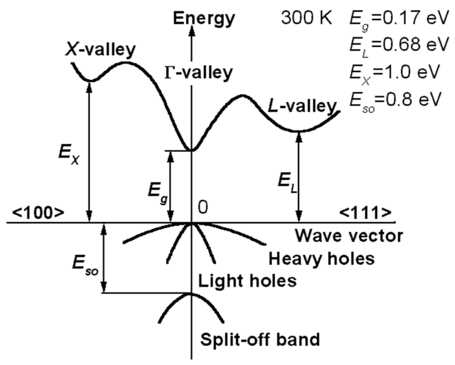
An indium antimonide crystal belongs to the O⁷_h symmetry group, which includes such “classical” semiconductors as Ge, Si, having a diamond-type lattice. This lattice is a face-centered cubic Г^f_c. It contains two identical atoms on the outside [30]. An indium antimonide crystal has p-type semiconductor holes, which are carriers of the current. In the valence band, Г8 (Г8 +) is formed —the zone of light and heavy holes (see Figure 1) and the Г₆ zone, which is split off from them due to the spin–orbit interaction, lies much lower and is completely filled [30,31].

Uniaxial deformation shifts the zone of heavy holes down. The wave functions of heavy holes in the lowest approximation in k (the first order of perturbation theory) are ${\psi }_{lk}=e^{i\overrightarrow{k}\overrightarrow{x}}{\displaystyle \sum _{m\text{'}=\pm 3/2,\pm 1/2}{c}_{m\text{'}}^l}(\overrightarrow{k}){\psi }_{m\text{'}}^{3/2}$, where the functions ${\psi }_{m\text{'}}^{3/2}$ are defined in the Luttinger–Kohn basis [30] in terms of Bloch functions for k = 0. The wave functions are written in the form of a spinor formally corresponding to the state of a particle with spin 3/2:

$${\psi }_{lk}=e^{i\overrightarrow{k}\overrightarrow{x}}\Vert \begin{array}{l}{c}_{3/2}^l(\overrightarrow{k})\\ c_{1/2}^l(\overrightarrow{k})\\ c_{-1/2}^l(\overrightarrow{k})\\ c_{-3/2}^l(\overrightarrow{k})\end{array}\Vert \equiv e^{i\overrightarrow{k}\overrightarrow{x}}{\Re }_{ik}$$

The matrix c is determined from the solution of the Schrödinger equation, which simultaneously determines the band spectrum. The transition to the diamagnetic state in a uniaxial deformed crystal was interpreted in [27,32] as an increase in the exchange interaction of holes at acceptors due to the splitting of the valence band in the presence of uniaxial compression. It was an assumption that for any values of the compression parameter, the ground state of the holes would be the level at which the spin vectors will be “antiparallel”, and with this, the energy gap between the impurity and valence bands will increase. In this case, the magnetic field induced a metallic state because the paramagnetic splitting of holes energy at acceptors becomes comparable with the width of the impurity band. However, we showed that the ground state of heavy holes in manganese-doped indium antimonide was not a simple “antiparallel”, but it was degenerate in the acceptor’s couple spin, which can have two values S = 0 and S = 2. Finally, the degeneracy was removed by the applied strong magnetic field, which in this case, induced a transition to a magnetic state with J = 2 and simultaneously a transition to a conducting state.

The spin Hamiltonian (54), which describes a system of particles with spins 3/2, contains nonlinear contributions from the square of the pair spin, the negative constant A of the exchange interaction of heavy holes, for the case of compression strain increases modulo. Thus, the gap between symmetric and antisymmetric states is growing, and equal to J = 2 | A | in the split zone of heavy holes, and the zone with heavy holes lowers, thereby increasing the width of the gap between the impurity levels and the states of heavy holes. The energy of the holes’ couple has the form (55). For evaluation, we assumed that the spin value of a pair was a continuously changing quantity, then we can establish some regularities in the behavior of the exchange contribution from the pair interaction of particles. Denote by x the value of the scalar product of two particle spins, where s = 3/2 and a “continual” total spin S as σ:

$$x=\frac{1}{2}\left(S(S+1)-2s(s+1)\right)=\frac{\left(2\sigma (\sigma +1)-15\right)}{4}.$$

The exchange contribution from pair interaction, measured in units of A as a function of a continuously changing variable x in the interval [−15/4, 9/4], is

$$y_{\frac{3}{2},\frac{3}{2}}=-\frac{2}{9}{x}^3-\frac{11}{18}{x}^2+\frac{9}{8}x+\frac{67}{32}$$

(63)

The dependence of the energy (63), measured in terms of the exchange interaction constant taking into account its sign, on the total spin σ is shown in Figure 2.

The energy correction of the holes couple E = K + A (see (55)) takes place at two values of the total spin σ = 0 and σ = 2 (both are the antisymmetric spin states). Thus, the exchange interaction removes the degeneracy in symmetry but does not completely remove the degeneracy in the total spin. In this case, the symmetric states of heavy holes displaced into the depth of the valence band, and the antisymmetric ones rose up, compensating for the influence of the deformation potential. The final removal of the degeneracy of the antisymmetric states, which determines the conductivity of heavy holes, occurred in a magnetic field. The Hamiltonian of the system in the magnetic field has the form:

$${\widehat{H}}_{\mathrm{int}}=K+A\left\{-\frac{2}{9}{\left(\frac{1}{2}\left({\widehat{S}}^2-2{\widehat{s}}^2\right)\right)}^3-\frac{11}{18}{\left(\frac{1}{2}\left({\widehat{S}}^2-2{\widehat{s}}^2\right)\right)}^2+\frac{9}{8}\left(\frac{1}{2}\left({\widehat{S}}^2-2{\widehat{s}}^2\right)\right)+\frac{67}{32}\right\}-B_{z}g{\widehat{S}}_z,$$

(64)

Here, B_z is the magnetic field directed along the compression axis of the sample, g is the gyromagnetic factor of the acceptor. Then the eigenenergy of the system in the magnetic field is

$$E=K+A\{-\frac{2}{9}{\left(\frac{1}{2}\left(\sigma (\sigma +1)-\frac{15}{2}\right)\right)}^3-\frac{11}{18}{\left(\frac{1}{2}\left(\sigma (\sigma +1)-\frac{15}{2}\right)\right)}^2+\frac{9}{8}\left(\frac{1}{2}\left(\sigma (\sigma +1)-\frac{15}{2}\right)\right)+\frac{67}{32}\}-B_{z}gM.$$

where $M$ is the total spin projection on the compression axis.

Thus, the antisymmetric states are split by the magnetic field into five sublevels with M = 2, 1, 0, −1, −2, where the state with M = 0 remains twice degenerate over the full spin with σ = 2 and σ = 0. Symmetric states are also split into seven sublevels, M = 3, 2, 1, 0, −1, −2, −3, where states with M = 1, 0, −1 remain twice degenerate over the full spin with σ = 1 and σ = 3.

5. Results and Discussions

When the magnetic field is switched on due to splitting, the sublevel with σ = 2 rises to impurity levels and changes the character of conductivity to metallic. The conductivity coefficient of a semiconductor due to scattering by impurities is determined by the expression:

$${\sigma }_{im}=\frac{e^2}{m{v}_{T}n\text{'}Q}{n}_0{e}^{-\frac{\Delta }{T}},$$

(65)

where $v_T=\sqrt{T/m}$ is the thermal velocity of the electron, l_ik = 1/n’Q is an electron mean free path taking into account scattering by impurities whose concentration is n’, and the cross-section is Q. The band gap Δ in pure indium antimonide is 0.2 eV, the band gap Δ’ between the impurity and valence band is an undeformed crystal ~ 0.04 eV. Upon compression, this gap increases due to an increase in both the absolute value of the exchange interaction and direct Coulomb repulsion: $\Delta {\text{'}}_{\chi }=\Delta \text{'}+K_{\chi }\pm \left|A_{\chi }\right|$, where the correction +|A| corresponds to the symmetric states σ = 1, 3, and the antisymmetric states σ = 0, 2 have the correction −|A|, both of which according to (65) reduce the conductivity. The splitting of impurity levels in a strong magnetic field leads to the fact that the down (symmetric) sublevel move into the valence band: $\Delta {\text{'}}_{\chi B}=\Delta \text{'}+K_{\chi }+\left|A_{\chi }\right|+MgB$, M = 3, 2, 1, 0, −1, −2, −3. For the antisymmetric sublevels, the gap is $\Delta {\text{'}}_{\chi B}=\Delta \text{'}+K_{\chi }-\left|A_{\chi }\right|+MgB$, where M = 2, 1, 0, −1, −2, the upper sublevels move into the conductive band since the gap between the impurity sublevel and the conductive band is almost leveled by the magnetic field: $\Delta {\text{'}}_{\chi B}=\Delta \text{'}+K_{\chi }-\left|A_{\chi }\right|-2gB\approx 0$. Thus, hole conductivity at the temperature of ~10 K increases by a factor of $\left|e^{\frac{\Delta {\text{'}}_{\chi }}{T}}\right|\approx 1\times e^7=1096$ which corresponds to the experimental results obtained in [33,34,35].

Indium antimonide crystals doped with manganese at impurity concentration around Ncr due to their exceptional physical properties can be used for advanced cryogenic devices operated in the millikelvin range of temperatures. The advantage of p-InSb(Mn) as athermosensitive material is that it is not restricted by the limitations of hopping processes at low and super-low temperatures, a quality which noticeably differs from the conventional Ge and Si semiconductors. In contrast to the conventional thermoresistors, p-InSb(Mn) resistance thermometers show exponential resistivity–temperature dependence described by Equation (65), where Δ varies between 0.007 and 1 meV. This unique property of p-InSb(Mn) crystals allows high thermosensitive materials with low specific resistivity in the millikelvin range of temperature to be obtained, thus reducing Pc. It was shown in [36,37] that the sensitivity of InSb(Mn) resistance at 10 mK reached aa value of ~1000 K⁻¹. Note that at T below 20 mK, Germanium thermoresistors practically lose their sensitivity as a result of the Variable range hopping (VRH) conductivity type.

We considered as the example of the high-spin system, the system of heavy holes, possessed by spin 3/2 and described its magnetic properties. Such consideration is actually also for the other high-spin systems. Theoretically, magnetic properties of the magnetic behaviors of the spin-1 nanostructures have been investigated successfully by using various techniques, such as MFT, EFT with correlations, MC simulations in the Ising model [38]. The equilibrium properties of nanostructures for the high spin system, such as 3/2, 5/2, and 2, are also the object of intensive studies. Such theoretical studies are useful for the analysis of the magnetic properties of nanoparticles, lyotropic liquid crystals, and the effects of spin ordering in liquid crystals and sensory systems. The scientific and practical significance of traditional liquid crystals built from organic molecules (mesogens) is well known. These molecules spontaneously, under the influence of dispersion forces and repulsive forces, combine into supramolecular ensembles, forming a liquid and, at the same time, ordered liquid crystal phase (mesophase) ordered by molecular orientations. Minimal external influence causes a change in the physical macroscopic properties of liquid crystals. It is the sensitivity of the liquid crystals to external factors that serves as the basis for their widespread use as a liquid but anisotropic medium in scientific research, in various devices for displaying and processing information (displays of computers and televisions, indicators, optical converters, etc.). At present, many laboratories in almost all developed countries are engaged in the synthesis and study of metallomesogens [39,40,41,42,43]. The first high-spin (S = 5/2) thermotropic liquid crystal was obtained—a mesogenic complex with a Fe(III) atom [44]. Synthesized polynuclear (homo- and heteronuclear) mesogenic complexes with a metal-containing ligand (derivative of ferrocene), including nematics with six iron atoms in their composition, have been obtained. The problem of creating mesogenic complexes of 3d elements with variable spin properties (high–low-spin transitions), i.e., search synthesis of systems combining liquid crystal and spin-crossover properties, is very important for the chemical sensors technology. Thus, mesogenic complexes of a number of lanthanides of the composition L3LnX3 with ligands from the class of azamethine compounds (Schiff base) and a wide range of counter-ionic ions were synthesized. Magnetic mesophases based on lanthanide complexes can be used to visualize magnetic fields of various surfaces, i.e., for magnetic flaw detection purposes. Of particular importance is the synthesis of a complex combining liquid crystal properties with the property to change the spin state depending on temperature. The study of such systems will allow, due to the sensitivity of the spin state to intermolecular interactions, the mechanisms of cooperative spin transitions to be detailed. Further efforts may lead to the use of such systems as chemical sensors.

Another application is ferrofluids. Ferrofluids are known as colloidal suspensions of ferromagnetic nanoparticles in aqueous or organic solvents. Dispersed particles are randomly oriented, but their moments are aligned when a magnetic field is applied, creating a variety of exotic and useful magneto-mechanical effects. Shuai et al. [45,46] reported that a liquid suspension of magnetic nanoplates spontaneously ordered into an equilibrium nematic liquid crystal phase, which is macroscopically ferromagnetic in this case. The barium hexaferrite (BF) nanoplates used in this experiment are suspended in isotropic n-butanol and surfactant-stabilized to produce a system of functionalized nanoplates with weak electrostatic repulsion, strong and anisotropic steric repulsion, and magnetic interaction. The magnetization in a zero field creates the characteristic magnetic effects of self-action, including the liquid crystal textures of the domains of liquid blocks located in closed loops of magnetic flux, which makes this phase highly sensitive, so much so that it changes shape sharply even in the Earth’s magnetic field. Such phases are possible because, in such hybrid suspensions, not only the energy of the magnetic dipole–dipole interaction between the supermolecular magnetic moments of neighboring particles but also the electric dipole–dipole exchange interaction, depending on the total spin of the particles, can be many times higher than the thermal energy at room temperature [47,48]. This BF nematic is distinctly ferromagnetic, with a magnetization density of two orders of magnitude larger than that reported in the previously found thermotropic nematic LC host (4-cyano-40-pentylbiphenyl, 5CB) fluid system [49]. The single-ion anisotropy for the system of ions with spin equals to 3/2 is relevant in accounting for the magnetic properties of a number of compounds: CsNiCl3 _weak axial anisotropy NENP [Ni(C₂H₈N₂₎₂NO₂(ClO₄)]weak axial anisotropy [8], CsFeBr₃, NENC [Ni(C₂H₈N₂)₂Ni(CN)₄], and DTN [NiCl₂−4SC(NH₂)₂]strong planar anisotropy [13]. Another exotic state—the spin nematic—has been discovered in the one-dimensional LiCuVO₄ [50,51,52]. The 3/2 Ising system was introduced to explain magnetic and crystallographic phase transitions in some compounds, such as DyVO₄, and then extended to describe tricritical properties in ternary fluids mixtures (ethanol–water–carbon dioxide) [53]. They presented a lattice-gas model of ternary fluid mixtures. Within the mean-field approximation, a nonsymmetric tricritical point is studied in this model. These theoretical results were compared to the experimental observations on the system ethanol–water–carbon dioxide.

The parameter of the exchange interaction is very important for considering spin statistics and spin dynamics in spin representation using the spin Hamiltonian. The exchange interaction, which determines the spin configuration, is the result of the Coulomb interaction of charges redistributed in real space in accordance with the state’s interference defined in the coordinate space and should be computed very carefully for the two particle’s interaction, while it represents a coupling constant for the consideration in the spin representation. Due to the unambiguous correspondence of the permutation relations for the coordinate and spin parts of the wave function, based on the fundamental principle of parity, a spin configuration is established that uniquely corresponds to the sign with which the Coulomb exchange interaction enters into the energy correction. In this sense, the main parameter determining the magnetic ordering in systems of identical particles is the exchange integral. The sign in front of the exchange integral in the expression of the total energy is determined by the parity of the permutation of the spatial part of the total wave function. Due to the unique connection with the parity of the spin part, this sign can be replaced by the operator in the spin representation, which contains “large degrees” of scalar products of spin operators’—biquadratic, bicubic, etc., сontributions with corresponding coefficients. Thus, the exchange interaction parameter determined by the integral exchange calculated in the coordinate representation is included in the resulting spin Hamiltonian as a common factor. The coefficients before the bilinear, biquadratic, bicubic, etc., terms are uniquely determined from the corresponding parity condition. Thus, the concept of a separate consideration of biquadratic or bicubic exchange interactions as various contributions, often used in theoretical papers devoted to the analysis of statistics of high-spin systems, becomes meaningless, since all the above contributions are determined by a unique, single parameter, namely, the exchange interaction integral calculated in the coordinate space. Depending on the real electronic configuration of the interacting atoms or molecules, this integral can be positive or negative or even change its sign depending on the change in the distances between the interacting particles. In this article, we have shown how, based on the first principles, based on the fundamental properties of the symmetry of angular momenta, we can obtain the exact shape of the spin Hamiltonian, which describes identical particles with a spin other than 1/2.