Article

Explaining Aggregated Recovery Rates

1
Assenagon Asset Management S.A., Zweigniederlassung München, Prannerstraße 8, 80333 München, Germany
2
Chair of Mathematical Finance, Technical University of Munich, Parkring 11, 85748 Garching, Germany
3
Rothesay, The Post Building, 100 Museum Street, London WC1A 1PB, UK
*
Author to whom correspondence should be addressed.
Risks 2022, 10(1), 18; https://doi.org/10.3390/risks10010018
Submission received: 10 September 2021 / Revised: 5 December 2021 / Accepted: 21 December 2021 / Published: 11 January 2022
(This article belongs to the Special Issue Quantitative Risk Measurement and Management)

Abstract

:
This study on explaining aggregated recovery rates (ARR) is based on the largest existing loss and recovery database for commercial loans provided by Global Credit Data, which includes defaults from 5 continents and over 120 countries. The dependence of monthly ARR from bank loans on various macroeconomic factors is examined and sources of their variability are stated. For the first time, an influence of stochastically estimated monthly growth of GDP USA and Europe is quantified. To extract monthly signals of GDP USA and Europe, dynamic factor models for panel data of different frequency information are employed. Then, the behavior of the ARR is investigated using several regression models with unshifted and shifted explanatory variables in time to improve their forecasting power by taking into account the economic situation after the default. An application of a Markov switching model shows that the distribution of the ARR differs between crisis and prosperity times. The best fit among the compared models is reached by the Markov switching model. Moreover, a significant influence of the estimated monthly growth of GDP in Europe is observed for both crises and prosperity times.

1. Introduction

The global financial crisis 2007–2009, which severely affected the world economies, showed the great importance of the appropriate calculation of credit risk in pricing financial contracts. The most important determinants of credit risk are default probability (PD) and recovery rate (RR) or Loss Given Default (LGD), i.e., 1 − RR. There are a couple of important reasons why those parameters should be taken into consideration. Firstly, they could be used to estimate the expected financial loss. Secondly, the estimations of PD and RR could help to determine an individual risk policy, e.g., if the values of the parameters are exceptionally high, more effort could be committed in order to mitigate the loss. Moreover, the financial risk of a portfolio, which is calculated using default probabilities and recovery rates, is essential for fulfilling the capital requirements of Basel accords.
The appearance of contingent claims on recoveries e.g., CDS (Credit Default Swap) as well as the variability and severity of the defaults during the financial crisis have shown the necessity to predict the recovery rates more precisely. We intuitively expect the recovery rate to be dependent on various factors: endogenous (characteristics of the lender and the conditions of the contract, e.g., rating, transaction amount, collateral) and exogenous (macroeconomic conditions, e.g., GDP (gross domestic product), unemployment or inflation rate). The modelling of recovery rates taking into consideration endogenous variables essentially started with Asarnow and Edwards (1995) and Altman and Kishore (1996). The first authors analyze US C&I (Commercial and Industrial) corporate loans and US structured loans and observe that structured loans have much higher RR than C&I loans. The latter examines the impact of collateralization, seniority and industry affiliation on individual recovery rates. Eales and Bosworth (1998) report that the size of the loan positively influences recovery rates for loan data in Australia. Carrizosa and Ryan (2013) and Donovan et al. (2015) find that creditors of firms with more conservative accounting prior to default have significantly higher recovery rates and Amiram and Owens (2021) show that accounting measures available to lenders at the contracting date are informative about future loss given default.
The influence of exogenous variables is examined e.g., by Altman et al. (2001), who find secondary effects of macroeconomic variables on annual recovery rates. Hu and Perraudin (2002) determine a negative correlation between the quarterly default rates and recovery rates. Jankowitsch et al. (2014) reach a more clear conclusion, which is also consistent with the result of Hu and Perraudin (2002). By examining US corporate bonds, they find that high default rates imply lower recoveries. Further, Bellotti and Crook (2012) shows that higher interest rates (measured by selected UK retail banks’ base interest rates) and higher unemployment at the time of default lead to lower recovery rates, but a higher earnings growth leads to increased RR. Surprisingly, Ingermann et al. (2016) claims that unemployment and inflation lead to an increase in recovery rates. Krüger and Rösch (2017) consider a quantile regression with endogenous as well as exogenous variables and show that this regression model outperforms the classical regression as well as its modification with a transformed response, beta regression, mixture regression with two components, and regression trees.
Most researchers agree that during economic downturns recovery rates are lower. Frye (2000) shows that during crisis times, RR might decline 20–25% with respect to prosperity times. Brumma et al. (2014) states that the economic situation at the date of the cash-flow weighted median of recovery payments has the highest impact on the recovery rate. Wang et al. (2020) also report that loan characteristics influence different recovery rates during good and bad times. Min et al. (2020) combine endogenous and exogenous variables together with crisis prediction during the average resolution time of 18 months to model individual recovery rates. They compare regression models as well as their combination with decision trees, neural networks, and mixture models. They found that the mixture regression model with regressed means of the components as well as with regressed probabilities provides the best fit among all considered models. This shows that the potential of regression models including crisis prediction as a regressor is not exhausted yet and that those models could serve as attractive competitors to modern machine learning methods. We refer to Qi and Zhao (2011) and Bellotti et al. (2021) for a comparison of machine learning techniques with regression methods.
Felsovalyi and Hurt (1998) consider 1149 defaults from 27 countries in Latin America over a time horizon of 27 years from 1970 to 1996. According to their empirical study, the recovery rates are higher for larger loans which are in contrast to Bastos (2010). Surprisingly, the authors claim that neither the economic fluctuations (measured by annual GDP growth of Latin America) nor the sovereign events affect RR. In contrast, Covitz and Han (2004) report a positive correlation between GDP and annually aggregated RR. Khieu et al. (2012) examine the determinants of bank loans recoveries using the “Ultimate Recovery Database”, a broad database supplied by Moody’s covering various debt instruments from the US defaulted companies. These authors report a positive impact of annual GDP growth on RR. From the more recent studies, Calabrese (2014) examines the impact of default rate, unemployment, and GGDP (annual growth of GDP from previous years) using data from the Bank of Italy’s Survey. Only the default rate turns out to be statistically significant, but the value of its coefficient is close to zero. Gambetti et al. (2019) consider a general class of beta regression models for bond recovery rates and investigate the impact of regressors on the shape of an underlying beta distribution. They also consider GDP for the US and linearly interpolate it for monthly observations. Depending on a considered model, they observe either a negative nonsignificant influence of GDP or a positive statistically significant one at a 1 % level.
Recently, several works propose interesting frameworks for modeling recovery rates. Sopitpongstorn et al. (2021) use nonparametric logit regressions with regression parameters depending on covariate values. A remarkable feature of this approach is its robustness with respect to distributional assumptions on the response variable, bimodality, and asymmetry. Candian and Dmitriev (2020) consider a dynamic stochastic general equilibrium (DSGE) model to explain fluctuation of recovery rates. Ye and Bellotti (2019) employ a beta mixture model combined with a logistic regression model. This is a two-stage model, which first fits a logistic regression to predict full recovery and then fits a beta mixture regression for recovery rates in an open unit interval. Fermanian (2020) models the joint distribution of default times and recovery rates using a Gaussian copula. In this way, he is able to quantify the influence of default probabilities on recovery rates in different scenarios of structural models.
In this article, we explain the behavior of monthly aggregated recovery rates (ARR) from the Global Credit Data (GCD) database using monthly and quarterly macroeconomic variables in a regression framework. The individual recovery rate of a specific loan is an important input variable for internal rating models but very hard to predict. In contrast, the ARR can be forecasted more significantly and may serve as a good proxy for an individual recovery rate. The database of GCD includes the default cases from 5 continents and over 120 countries. GCD was formed in December 2004 as a credit risk data-pooling initiative primarily designed to assist member-banks in enhancing their internal credit risk models, completing the Basel II preparations in pursuit of the International Ratings Based Advanced Status, and improving their risk assessment for risk and credit portfolio management purposes. Since then, GCD has enjoyed remarkable success, both in terms of growing its membership and establishing its international reputation through the creation of the largest existing loss and recovery dataset for commercial loans worldwide.
Previous studies are restricted to quarterly or annual GDP growth. We first model monthly ARR using monthly signals extracted from quarterly GDP derived from other monthly macroeconomic variables. For this, we consider a dynamic factor model for mixed-frequency panel data and estimate them as described in Banbura and Modugno (2014). Keijsers et al. (2018) also consider a similar factor model to couple individual recovery rates, three macroeconomic variables including GDP, and individual characteristics of loan and borrower. They are able to explain the cyclicality in recovery rates and default rates driven by latent factors for all observed variables. In contrast, we consider the ARR and do not mix it with macroeconomic variables. Further, we consider 19 (34) macroeconomic variables for Europe (US) to estimate monthly GDP growth rates from quarterly GDP growth rates. Using the estimated factors, we are especially able to quantify an undisturbed influence of GDP on monthly ARR. In order to improve the regression fit, shifts of covariates in time are considered. A Markov switching model with two states is applied to show that the distribution of the ARR and their dependence on explanatory variables may vary between different states.
The structure of the article is as follows. In Section 2, the derivation of monthly estimates of GDP growth using a dynamic factor model for mixed-frequency data is presented. A description of the general idea of dynamic factor models and panel data is given in Appendix A. In Section 3, the explanatory variables for the regression models are introduced. Section 4 presents several regression models for the ARR. Here, we apply time shifts to explanatory variables and combine a linear regression with a Markov switching model. Section 5 summarizes and concludes the paper.

2. Estimating Monthly GGDP

We model monthly aggregated recovery rates using monthly and quarterly observed data. In particular, the GDP in Europe and in the US is released only on a quarterly basis. A rather naive approach to derive monthly estimates out of quarterly data is a linear interpolation. In this paper, we will apply a dynamic factor model to estimate the monthly growth of the GDP (GGDP). The monthly GGDP is observed at a particular month if this month is the last month of a quarter. It is then computed as a log-return of the GDP assigned to the quarter of the considered month and the GDP of the previous quarter. For the first and second months of a quarter, the GGDP is missing. A detailed description of the model can be found e.g., in Banbura and Modugno (2014).
As input data in our factor model, we use a data set containing quarterly GDP as well as many other monthly and quarterly observed economic variables describing the macroeconomic environment, interest-rate movements, and stock-markets behavior. The list of variables can be found in Appendix A. The GCD data, which was available to us, covers the period from January 2000 until January 2014. For quarterly variables like GDP, only every third observation is available and other values are missing. Out of this mixed frequency data, we derive the factors which will be used for modeling the ARR.
Similar to Banbura and Modugno (2014), we use transformations of the variables instead of the original data. We take the difference of consecutive observations or the difference of the logarithms of consecutive observations to make the observed time series stationary. In the case of the European GDP and the US GDP, we transform the variables by taking the difference of logarithms, which results in quarterly log returns. Our goal is to reconstruct monthly time series from the quarterly growth of GDP for Europe and the US using dynamic factor models. The considered mixed frequency panel data sets are similar to those in Schumacher and Breitung (2008), who were estimating the GDP of Germany.
In the case of Europe, the quarterly GDP data and most of the other observable variables used for the estimation are average values of 19 European countries. The derived GGDP will also be the estimation of the average GGDP of those countries. For the European GGDP estimation, 29 variables are used and the data is almost entirely taken from the website of the European central bank (http://sdw.ecb.europa.eu/, accessed on 31 March 2017). Only the VSTOXX volatility index observations are taken from a different source. Those are available at https://www.investing.com/indices (accessed on 5 April 2017). The data used for estimating the US GGDP consists of 34 variables and is available on the webpage of the Research Division of the Federal Reserve Bank of St. Louis (https://fred.stlouisfed.org/ accessed on 27 March 2017).

2.1. Estimation with Dynamic Factor Models

The main idea of a factor model is to derive a few unobserved (latent) factors, which describe the behavior of high-dimensional data. The model consists of two equations. The first is the observation equation, which explains the relation between observation vector y t R n and the latent factors f t R q for t { 1 , 2 , , T } . It has the following form:
y t = W f t + e t for t = 1 , 2 , , T ,
where W R n × q , e t R n is a normally distributed error term with e t N ( 0 n , D ) , and D R n × n is a diagonal matrix.
The second equation is called state or transition equation. It describes the dynamics of the unknown factors f t over time. We assume that f t follows a vector autoregressive model of order p:
f t = A 1 f t 1 + + A p f t p + u t = A f ¯ t 1 + u t ,
where f ¯ t 1 : = [ f t 1 , f t 2 , , f t p ] R p q , A : = [ A 1 , , A p ] R q × p q is a parameter matrix, u t is a normally distributed and independent white noise error term with u t N ( 0 q , Q ) for t { 1 , 2 , , T } , Q R q × q . The whole available data is centralized, i.e., the mean of the time series was subtracted. We define Y : = ( y 1 , y 2 , , y T ) R n × T and F : = ( f 1 , f 2 , , f T ) R q × T .
For the European and the US GGDP, we obtain monthly estimates by treating quarterly growths as monthly data with missing values. In the observation vector y t , the missing values are denoted by NA. To deal with the incomplete data, Banbura and Modugno (2014) suggested introducing a diagonal matrix M t with 0 on the diagonal if the corresponding observation is missing and 1 if the observation is available. Using the matrix M t , we can split the observation vector y t into two parts, one corresponding to observed values and one corresponding to missing values:
y t = M t y t + ( I n M t ) y t ,
where I n denotes the identity matrix of dimension n. Hence, the vector M t y t does not contain any missing values denoted by NA any more. Due to the diagonal structure of D, the log-likelihood function of the dynamic factor model (1)–(2) can be integrated with respect to f t and e t and depends on the matrix M t . For details, we refer to Banbura and Modugno (2014).
The parameters θ : = ( A , W , D , Q ) are unknown and need to be estimated. As in Defend et al. (2021), we choose A ( 0 ) = 0 q × p q for an initial estimate of A and for an initial estimate of Q we choose Q ( 0 ) = I q . The initial values D ( 0 ) and W ( 0 ) are calculated according to a probabilistic principal component analysis (see Tipping and Bishop (1999)). Having the initial estimates, we proceed with the estimation using the expectation-maximization algorithm (see Dempster et al. (1977)). The main idea of the algorithm is to write the log-likelihood as if the data ( Y , F ) was complete and to iterate between the expectation and maximization steps. In the expectation step, we take the expectation of the log-likelihood function L ( θ | Y , F ) , which is dependent on the unknown model parameters θ given the data ( Y , F ) , under the current j estimate θ ( j ) of the parameters given Ω T , the observations available up to time T. As in our situation, some observations are missing, Ω T does not contain every value from Y. In the maximization step, we compute the maximum of the just calculated expected log-likelihood function to derive the maximum likelihood estimates of θ under the current estimates of θ ( j ) . The steps of the algorithm are as follows:
  • Expectation step (E-step):
    Θ ( θ | θ ( j ) ) = E θ ( j ) [ L ( θ | Y , F ) | Ω T ] ,
  • Maximization step (M-step):
    θ ( j + 1 ) = arg max θ Θ ( θ | θ ( j ) ) .
As derived in Banbura and Modugno (2014), the parameter estimates after the ( j + 1 ) th iteration have the following form:
A ( j + 1 ) = t = 1 T E θ ( j ) [ f ¯ t f ¯ t 1 | Ω T ] t = 1 T E θ ( j ) [ f ¯ t 1 f ¯ t 1 | Ω T ] 1 ,
v e c ( W ( j + 1 ) ) = t = 1 T E θ ( j ) [ f ¯ t f ¯ t | Ω T ] M t 1 v e c t = 1 T M t y t E θ ( j ) [ f ¯ t | Ω T ] ,
D ( j + 1 ) = d i a g ( 1 T t = 1 T ( ( I n M t ) D ( j ) ( I n M t ) + M t y t y t M t M t y t E θ ( j ) [ f ¯ t | Ω T ] W ( j + 1 ) M t M t W ( j + 1 ) E θ ( j ) [ f ¯ t | Ω T ] y t M t + M t W ( j + 1 ) E θ ( j ) [ f ¯ t f ¯ t | Ω T ] W ( j + 1 ) M t ) ) ,
Q ( j + 1 ) = 1 T t = 1 T E θ ( j ) [ f ¯ t f ¯ t | Ω T ] A ( j + 1 ) E θ ( j ) [ f ¯ t 1 f ¯ t | Ω T ] .
In Equation (3), ⊗ denotes the tensor product. The above estimators depend on the conditional moments E θ ( j ) [ f ¯ t | Ω T ] , E θ ( j ) [ f ¯ t 1 f ¯ t | Ω T ] , E θ ( j ) [ f ¯ t f ¯ t | Ω T ] and E θ ( j ) [ f ¯ t 1 f ¯ t 1 | Ω T ] . To estimate them, we use the Kalman filter and Kalman smoother (see, e.g., Nakata and Tonetti (2010). The estimators of the latent factors f t are then given by
f ^ t | T = [ I q 0 q × ( p 1 ) q ] f ¯ t | T s = ( f ¯ t | T s ) [ 1 : q ] ,
where f ¯ t | T s is an estimator of f ¯ t using the Kalman smoother based on the whole available information Ω T . The termination criterion ζ is defined after Doz et al. (2011) and stops the iteration procedure if
ζ = L ( θ ( j ) | Y , F ) L ( θ ( j 1 ) | Y , F ) ( L ( θ ( j ) | Y , F ) + L ( θ ( j 1 ) | Y , F ) ) / 2 < 0.001 .
Since factor dimension q and autoregressive order p are not known, we estimate the model (1) and (2) for different combinations of q and p. We considered the five following combinations of parameters ( q = 1 , p = 1 ), ( q = 2 , p = 1 ), ( q = 3 , p = 1 ), ( q = 2 , p = 2 ), ( q = 3 , p = 2 ) and decided to choose the model, whose estimates provide the best fit in a linear regression for aggregated recovery rates (see Section 4). According to this criterion, in case of the European GGDP the dynamic factor model with parameters ( q = 2 , p = 2 ) is the best and for the US GGDP the one with ( q = 2 , p = 1 ).

Estimators of Missing Data

In the dynamic factor model, we derive the latent factors using the observed data. In order to derive the monthly estimators of missing data, we perform the opposite operation. Thus, we calculate the estimator Y ^ = ( y ^ 1 , y ^ 2 , , y ^ T ) of data Y using f ^ t | T and an estimator W ^ of W by
y ^ t = W ^ f ^ t | T .
The above equation is the observation equation with the neglected error term. The fitted data has no missing values and we get the estimator of the GGDP from the appropriate column of matrix Y ^ . In Figure 1 and Figure 2, we present the original quarterly data and the estimated monthly values of the GGDP for Europe and the US, respectively.
From Figure 1 and Figure 2, we clearly see that the estimators of the GGDP are different compared to the estimators obtained by linear interpolation. In contrast to the linear interpolation, where only the GDP values observed every quarter matter and other monthly fluctuations in the economy within those 3-months periods are completely neglected, our estimates reflect the information about changes in the economy contained in the broad data set used for estimation of the dynamic factor model. In the linear interpolation, we need to know the first and last observation of the considered period to estimate the values in between and thus this is a forward-looking estimation. In contrast to the linear interpolations, we do not use the observed, quarterly values, but the corresponding fitted monthly values. Especially, we expect that the estimated GGDP will let us predict the behavior of the aggregated recovery rates better. This statement is examined in the next section.
In the literature, a special case of factor models, called static factor models, is also used. In a static framework latent factors are assumed to be independent, State Equation (2) is omitted and the model is given by Equation (1) only. We have also estimated the European GGDP and US GGDP using the static factor model (for q = 1 , 2 , 3 ). However, the corresponding estimators of the GGDP have less explanatory power for aggregated recovery rates than the ones resulting from the dynamic model, which are presented in Figure 1 and Figure 2.

3. Data for Regression Models

The recovery rates are taken from the Loss Given Default (LGD) database of GCD (formerly known as Pan-European Credit Data Consortium or PECDC). Global Data Consortium was founded by 13 European banks to provide a collection of historical loss data, analysis, and research resources to contribute to a better understanding of credit risk. The database contains over 110,000 individual facility default records from over 50,000 obligors over a period from 1990 to date. The data is collected on the basis of 11 distinct asset classes (all except retail), which mirror those defined in the Capital Requirements Directive. The more than 50 member-banks are from Europe, Africa, Asia, Australia, and North America. This is also reflected in the geographical coverage of the database which, originally limited to Europe, has been extended to include global exposures and the records from over 120 countries.
The database available to us includes the loss data from the period 1990–2014. The defaults from the years 2012–2014 are partially unresolved and the banking regulations before 2002 were significantly different. Therefore, we analyze the data from 2002 till the end of 2011 in our study. This period covers more than one full economic cycle as postulated in §472 of the Basel Committee on Banking Supervision (2004).
The other variables used in the regression models, 1-month Euro Interbank Offered Rate (EURIBOR: 1M), 3-months Euro Interbank Offered Rate (EURIBOR: 3M), industrial production of European countries (Production), 5-year Euro area Government Benchmark Bond yield (GY), average inflation of European countries (Inflation) and average unemployment of European countries (Unemployment) are taken from the website of the European central bank (http://sdw.ecb.europa.eu/, accessed on 31 March 2017). The VSTOXX volatility index, Dow Jones Euro STOXX 50 (STOXX 50), and S&P500 are available at https://www.investing.com/indices, accessed on 5 April 2017. In the case of Production, Inflation, and Unemployment the data concerns 19 European countries.

3.1. Recovery Rates

The recovery rate is usually defined as the fraction of the exposure at default (EAD) that is recovered from a defaulted entity. The recovery rate could be also defined as 1 − Loss Given Default (LGD). More information on the definition of default and estimation of LGD can be found in the guidelines EBA/GL/2016/07 (2016) and EBA/GL/2017/16 (2017) of the European Banking Authority. According to the EBA/GL/2017/16 (2017), the workout LGD, i.e., losses computed using discounted cash-flows during a workout process, based on the institution’s experience in terms of recovery processes and losses is considered to be the main, superior methodology that should be used by institutions. Therefore, in this paper, we use the workout method to calculate the LGD as provided by the GCD.
Since we are only interested in real losses, all facilities for which the default amount is 0 were excluded from our database. Furthermore, in order to exclude all cases with unreasonable cash flows and the cases which are not fully resolved, we exclude all entities for which the total sum of reported cash flows (including chargeoffs and waivers which are not present in the calculation of economic recovery rates) divided by the outstanding amount at default is smaller than 90% or greater than 105% of the outstanding amount at default. In order to exclude exceptionally low or high recoveries, we remove observations with recovery rates outside the interval [ 0 , 1 ] . Those situations are possible because of costs and fees associated with recovery rates. Note that this sample selection is in line with Krüger and Rösch (2017) and Keijsers et al. (2018).
Table 1 presents some basic statistics of the recovery rates. In the column “Weighted”, the statistics are computed by using the default amount as weight. “Simple” statistics are, in contrast, equally weighted. The figures in both cases are similar.
Therefore, we decided to use equally-weighted recovery rates. Figure 3 shows the distribution of the resulting recovery rates. Thus, we can conclude that the distribution is bimodal.
The same observation has been made by Asarnow and Edwards (1995); Schuermann (2004); Bastos (2010); Calabrese (2012) or Ingermann et al. (2016). For defaulted bonds, Carty and Lieberman (1996); Carty et al. (1999); Hu and Perraudin (2002) or Jankowitsch et al. (2014) have observed unimodal or at least less skewed distributions.

3.2. Explanatory Variables

To model the monthly aggregated recovery rates, we use the European GGDP (GGDP Europe), the GGDP of United States (GGDP USA), average inflation of European countries (Inflation), average unemployment of European countries (Unemployment), industrial production of European countries (Production), 1-month Euro Interbank Offered Rate (EURIBOR: 1M), 3-months Euro Interbank Offered Rate (EURIBOR: 3M), 5-year Euro area Government Benchmark Bond yield (GY), S&P500, Dow Jones Euro STOXX 50 (STOXX 50) and VSTOXX volatility index (VSTOXX). The first five variables describe the macroeconomic environment, the following three refer to interest-rate movements and the last two are proxies for stock market behavior. The 1-month and 3-months European interbank offered rates (EURIBOR) serve as proxies for the short-term interest rates in the Eurozone, GY is calculated as the weighted mean of bond yields with maturities between 4.5 and 5.5 years, with default amount as weight, the Dow Jones STOXX 50 and S&P500 are proxies for equity markets and eventually, VSTOXX is a volatility index calculated from the implied volatilities of STOXX 50.
The impact of all those variables on the recovery rates is rather small when we consider every default individually. Figure 4 shows the average recovery rate computed for every percentile of the considered explanatory variables. None of the variables shows any significant correlation with recovery rates. Our observations are consistent with Grunert and Weber (2005); Dermine and Neto De Carvalho (2006) or Calabrese (2014) who did not find any dependencies between exogenous variables and RR on the unaggregated level. The exogenous explanatory variables become much more important when we consider monthly aggregated recovery rates, i.e., equally-weighted monthly averages of recovery rates based on the default date. We will examine the monthly aggregated recovery rates in the next section.

4. Aggregated Model

4.1. Linear Regression

We start with linear regression. The response variable is the monthly aggregated, equally-weighted average of the recovery rates based on the default date:
A R R ( t i ) = 1 n i j = 1 n R R j · 𝟙 ( D D j t i ) ,
where R R j denotes the recovery rate, D D j the default date of the jth entity, j = 1 , , n , t i the i-th month of our data set and n i is the number of the defaults in the i-th month. We choose the monthly averages in order to reduce random noise, which is present in smaller time frames like daily data and to assure that the sample is sufficiently large at the same time.
We assume a linear relationship between the logarithm of the aggregated recovery rates and the explanatory variables:
ln ( ARR ( t ) ) = β 0 + β 1 GGDP Europe ( t ) + β 2 GGDP USA ( t ) + β 3 Inflation ( t ) + β 4 Unemployment ( t ) + β 5 Production ( t ) + β 6 EURIBOR : 1 M ( t ) + β 7 EURIBOR : 3 M ( t ) + β 8 S & P 500 ( t ) + β 9 STOXX 50 ( t ) + β 10 VSTOXX ( t ) + β 11 GY ( t ) + ϵ ( t ) .
The estimated model is presented in Table 2. Its coefficient of determination R 2 and adjusted coefficient of determination R a d j 2 are 52.8 % and 47.9 % , respectively. EURIBOR: 1M, EURIBOR: 3M, Inflation rate, GY, Production, and GGDP USA are significant at the 5 % level.
In order to avoid the impact of possible multi-collinearity and to find the most important explanatory variables, we apply the backward-forward model selection procedure with AIC as a selection criterion (see, e.g., Draper and Smith (1998)). In the resulting estimated model (see Table 2), all previously mentioned variables are still significant at the 5 % level and the others are discarded from the model by the model selection procedure. The explanatory power of the model does not change significantly, R 2 and R a d j 2 remain at a similar level as for the initial model. As expected, GGDP USA, Production, and GY have a positive influence while Inflation has a negative influence on the aggregated recovery rate. Euribor:3M and Euribor:1M have an opposite influence on the aggregated recovery rates. This might be an indication that, the more convex the term structure, the lower the aggregated recovery rates.
For comparison, we have examined the model with the GGDP estimated using a linear interpolation instead of a dynamic factor model. Before backward-forward selection, this model yields R 2 = 50.93 % and R a d j 2 = 45.93 % . After the selection procedure, neither GGDP Europe nor GGDP USA is part of the reduced model. Further, its R 2 = 47.55 % and R a d j 2 = 44.76 % indicate that our reduced model still describes the behavior of the ARR better.

4.2. Model with Time Shifted Covariables

The success of a restructuring effort or the liquidation of collaterals does not realize immediately at the default of a borrower, but somewhere in the time span between default and resolution (usually about two years on average). Thus, the economic situation at some point after the default may be more significant for the recovery rates than the situation at the time of default. Therefore, we will examine how a modification of the explanatory variables with some form of time-shift affects the model fit. The topic of time shifts was also discussed in the literature. Carey and Gordy (2004) stated that the conditions one year after default matter more than the conditions just after default. Brumma et al. (2014) used the median of the cash-flow weighted time to resolution as time shift. Cash-flow weighted time can be different for different borrowers as it is related to the time point when all recovery cash flows are realized. According to Brumma et al. (2014), it is 12–18 months after default on average.
Figure 5 and Figure 6 display some explanatory variables against the aggregated recovery rates in order to examine their mutual dependence with the ARR. For the majority of variables except for VSTOXX and unemployment, we observe a strong positive correlation. We also find that time shifts can lead to even higher levels of correlation for most of the variables.

4.2.1. Optimal Time Shifts

We find an individual optimal time shift for every explanatory variable in such a way that it yields the highest absolute correlation between the considered variable and the recovery rate. For this, we consider all possible full-month time shifts from the interval [ 0 , 24 ] and for every explanatory variable we are looking for the solution to the following problem:
arg max | cor A R R ( t ) , v a r i a b l e ( t + i ) | for i { 0 , 1 , , 23 , 24 } .
In Table 3, the optimal time shifts in months for all variables and corresponding correlations are presented.
We observe rather large time shifts for the interest-rate proxies: EURIBOR: 1M, EURIBOR: 3M, and GY. Those variables are strongly correlated with interest rates set up by central banks, e.g., FED. Central banks usually do not change their rates more often than once in a quarter and the changes are very rarely higher than 0.5 percentage points. Therefore, the interest rates 18 months or 12 months after the default could reflect the economic situation related to the default much better. As terminating employees’ contracts is a long process, another very slowly changing variable is Unemployment (18 months). A large, 12-months time shift seems to be appropriate for Inflation since price changes are in most cases very slow. It is also easy to interpret the large time shift for Production (10 months). The production processes are usually planned in advance in order to assure an appropriate supply of necessary materials, intermediate products, and labor supply as well as to meet the orders of merchants. Thus, the delay in responding to a changing economic situation is significant. The reaction of stock markets is usually believed to be fast, but S&P500 and STOXX 50 comprise stocks of very different companies, which also react differently to the changes on the market and therefore a 6-months shift in the case of both indexes seems to be appropriate. GDP is released quarterly and usually reflects very quickly the condition of the economy. Therefore, 2 and 0 month shifts for the European and US GGDP, respectively, is not surprising. Finally, the volatility in the market is changing very dynamically, and not applying any time shift for this explanatory variable is economically reasonable. The relation between the optimally-shifted covariables and the aggregated recovery rates is presented in Figure 7 and Figure 8.
To model the ARR with covariates shifted in time, we assume a linear relationship between the logarithm of aggregated recovery rates and the explanatory variables in the following model
ln ( ARR ( t ) ) = β 0 + β 1 GGDP Europe ( t + 2 m o n t h s ) + β 2 GGDP USA ( t ) + β 3 Inflation ( t + 12 m o n t h s ) + β 4 Unemployment ( t + 18 m o n t h s ) + β 5 Production ( t + 10 m o n t h s ) + β 6 EURIBOR : 1 M ( t + 18 m o n t h s ) + β 7 EURIBOR : 3 M ( t + 18 m o n t h s ) + β 8 S & P 500 ( t + 6 m o n t h s ) + β 9 STOXX 50 ( t + 6 m o n t h s ) + β 10 VSTOXX ( t ) + β 11 GY ( t + 12 m o n t h s ) + ϵ ( t ) .
The model with shifted variables leads to a much higher coefficient of determination and adjusted coefficient of determination than the model without shifts (see R 2 = 71.1 % and R a d j 2 = 68.2 % given in Table 4). S&P500, STOXX 50, and GGDP Europe are significant at the 5% level. Some coefficient signs are not consistent with the correlations from Table 3 due to multicollinearity. In order to determine the most important explanatory variables, we perform a backward-forward model selection procedure using AIC as the selection criterion. This leads to the following model:
ln ( ARR ( t ) ) = β 0 + β 1 GGDP Europe ( t + 2 m o n t h s ) + β 2 Unemployment ( t + 18 m o n t h s ) + β 3 S & P 500 ( t + 6 m o n t h s ) + β 4 STOXX 50 ( t + 6 m o n t h s ) + ϵ ( t ) .
The results of the linear regression before and after the backward-forward model selection procedure are presented in Table 4.
The reduced model (6) has similar values of R 2 and R a d j 2 as model (5). All explanatory variables in this model are significant at the 5% level. The coefficients of S&P500 and GGDP Europe are positive and the coefficient of the Unemployment rate is negative. This indicates that the higher the value of S&P500 or GGDP Europe the higher the recovery rate and the higher the unemployment rate the lower the aggregated recovery rates. The negative sign of the coefficient of STOXX 50 is somehow surprising. However, if this variable is considered together with S&P500 (both are the indicators of stock markets), their joint effect on aggregated recovery rates is positive.
We measure this joint influence over time by mutually increasing their values by 1%. The corresponding sensitivity (change/difference) of the logarithmized RR is presented in Figure 9. We see that the joint effect on aggregated recovery rates is always positive. Another interesting finding is that the influence of the stock markets is relatively higher in prosperity times and lower in crisis times.
Similar to the model with unshifted explanatory variables, the above two models based on the stochastically estimated GGDP Europe and GGDP USA outperform the corresponding ones with linearly interpolated GGDP Europe and GGDP USA in terms of R 2 and adjusted R a d j 2 . The estimation accuracy of Model (6) is presented in Figure 10, where the fitted values are plotted together with the observed values. Model (6) seems to fit the ARR very well since the estimated and observed ARR are very close to each other.
Besides the linear model with logarithmized response variable, different regression models were utilized to find a model with the best fit. Thus, we considered linear regressions with a beta, logit, and probit transform as well as beta regression. None of the models gives better results than the linear regression (5), but the four models lead to similar conclusions. We observe positive correlations for EURIBOR: 3M, S&P500, GY, and GGDP USA with the aggregated recovery rates and negative correlation for EURIBOR: 1M. After the backward-forward selection, the regression model (6) still outperforms the above four linear regressions.

4.2.2. Applying the Same Time Shifts for All Variables

Now, we will examine the models with the same time shifts applied to all explanatory variables. In Table 5, the adjusted R a d j 2 is reported for the models without shifts, with 6 and 12-months shifts as well as with the individual optimal shifts, as discussed in the previous subsection for comparison.
In Figure 11, we also present the prediction errors for each of the models with different time shifts.
The models with 6-months and 12-months time shifts for all explanatory variables have higher R a d j 2 and lower standard deviation than the unshifted model, but still lower R a d j 2 and higher standard deviation than the model with optimal shifts. Therefore, in the upcoming three subsections, we will use the optimally time-shifted variables.
We should keep in mind that it is not possible to obtain such a high precision of prediction at the time of default as in the models with shifted variables. The required data is not available in time. For example, in our model with optimal shifts, we need information up to 18 months into the future. Therefore, it is essential to introduce an approach, which allows us to get predictions at the time of default. We present here an approach, which uses the empirical distribution of the explanatory variables.

4.2.3. Approach Using the Empirical Distribution

As basis for the empirical distribution, we use the 120 last observations. First, we calculate for any point in time k the vectors containing the differences for the 4 explanatory variables from Model (6):
δ i j = x i j x i ( j o p t ( i ) ) ,
where x i j is the jth observation of variable i with i { 1 , 2 , 3 , 4 } , j { k 120 , k 119 , , k 1 } , and o p t ( i ) is the optimal shift for variable i. Then, for any point in time k, we estimate 120 recovery rates by inserting the vectors x 1 , k + δ 1 , j , , x 4 , k + δ 4 , j in Model (6) and compute the 99 % prediction interval for those estimates.
The calculated prediction interval together with the mean of the predictions and the observations are presented in Figure 12. Only 3 observations out of 144 fall out of the interval (2.08%), which indicates good precision.
The above method could also be used when we calculate the predictions of the recovery rate not only right after default, but at later points in time. In this situation, we take advantage of the fact that more information might be already available at later points and use exact values instead of distributions where the covariates are already known. We expect that the empirical distribution of the differences in the covariates has lower variance and therefore we expect the prediction interval to become tighter.
We extend our approach by computing the prediction intervals for the time points 3, 6, 9, and 12 months after default. The idea of the method stays the same. The results are presented in Figure 13 and Figure 14.
As expected, the prediction intervals become tighter and tighter if more time has passed since default. However, the coverage of the predictions intervals becomes less accurate for larger shifts in time. Thus, there is a trade-off between tightness and precision of the prediction intervals for longer time after default.

4.3. Linear Model with Interactions

In this subsection, we try to improve the prediction power of Model (6) by introducing interactions. The model with the original four factors and all their possible two-factor interactions consists of 10 variables and leads to a coefficient of determination R 2 = 73.4 % and an adjusted coefficient of determination R a d j 2 = 70.9 % . As before, we apply the backward-forward model selection procedure in order to select important interactions. The obtained model has the following form:
ln ( ARR ( t ) ) = β 0 + β 1 Unemployment ( t + 18 m o n t h s ) + β 2 S & P 500 ( t + 6 m o n t h s ) + β 3 STOXX 50 ( t + 6 m o n t h s ) + β 4 GGDP Europe ( t + 2 m o n t h s ) + β 5 Unemployment ( t + 18 m o n t h s ) * S & P 500 ( t + 6 m o n t h s ) + β 6 Unemployment ( t + 18 m o n t h s ) * STOXX 50 ( t + 6 m o n t h s ) + β 7 S & P 500 ( t + 6 m o n t h s ) * GGDP Europe ( t + 2 m o n t h s ) + β 8 STOXX 50 ( t + 6 m o n t h s ) * GGDP Europe ( t + 2 m o n t h s ) + ϵ ( t ) .
The estimation results for the models before and after the selection are presented in Table 6. Note that the reduced model has similar R 2 and R a d j 2 .
Incorporating interactions allows to explain the behavior of aggregated recovery rates better, but even more interesting than this gain in degree of explanation is the possibility to have a closer look at the interdependence between the explanatory variables. In the estimated reduced model from Table 6, the coefficients of S&P500 and STOXX 50 have opposite signs as compared to Model (6). Further, the impact of the factors on the aggregated recovery rates depends now on other factors as well and the interpretation of the estimated coefficients is not straightforward anymore.
Similarly, as in the case of Model (6), we assume growth of 1 % of the considered variable, use monthly values of the remaining variables, and investigate the sensitivity of the logarithmized recovery rates over time. The results are presented in Figure 15 and Figure 16.
The impact of S&P500 on recovery rates depends on Unemployment and GGDP Europe, but it is still clear and intuitive. An increase in S&P500 in all possible economic conditions leads to an increase in recovery rates. The interpretation is also clear for Unemployment. The growth of this variable has a negative effect on the aggregated recovery rates in all possible economic conditions. The impact of STOXX 50 on logarithmized ARR is less intuitive. Except for two short time periods at the beginning of 2006 and at the end of 2008, an increase in STOXX50 leads to lower aggregated recovery rates. However, if the impact of STOXX50 is considered together with the impact of S&P500, the joint effect of those two variables has a positive impact on ARR in all economic conditions. This effect is shown in Figure 17.
From Figure 15 and Figure 16, we can also see that the impact of the explanatory variables changes over time. The influence of GGDP Europe is low in crisis times and gets higher in prosperity times. The opposite behavior could be observed for Unemployment. The impact of this variable is bigger in crisis times. To investigate this changing influence of the variables, we consider a Markov switching model in the next section and examine the data separately in crisis and prosperity times.
Using the empirical distribution approach, we calculate the prediction intervals for the reduced model from Table 6 as it was done for Model (6). The results are presented in Figure 18. The obtained prediction intervals are tighter than ones for Model (6). Only 1 observation out of 144 (0.69%) falls out of them, which indicates a higher precision.

4.4. Markov Switching Model

In this subsection, we consider two stochastic processes in discrete time. The first one, ( S t ) t N 0 , is an unobservable Markov chain with several states, i.e., its state space is Ω = { 1 , 2 , , r } . The second stochastic process, ( Y t ) t N 0 , is observable and we assume its distribution to be normal. In our analysis, the observable process is represented by the logarithmized aggregated recovery rates ln ( A R R ( t ) ) .
The distribution of ( Y t ) t N 0 depends on the unobservable state of the Markov chain. We denote the transition matrix of the Markov chain by Π = ( π j l ) j , l = 1 , , r , where π j l = P ( S t = l | S t 1 = j ) and the initial distribution by δ , with δ = δ ( s ) = P ( S 0 = s ) for s = 1 , , r . The probability density of ( Y t ) t N 0 given the particular state of ( S t ) t N 0 we denote by:
p ( s , y ) = P ( Y t = y | S t = s ) = 1 2 π σ s 2 exp ( y μ s ) 2 2 σ s 2 ,
where μ s and σ s are the state-dependent distribution parameters with s { 1 , 2 , , r } .
First, the initial distribution, transition matrix, and the parameters of the distribution are estimated. A very common approach to do this is the Baum-Welch algorithm (Baum et al. (1970)). Second, we need to determine the number of states r. Since the estimation results for the models with r = 3 and r = 4 are not stable, i.e., heavily dependent on the initial values, we proceed in our analysis using a model with two states and call these states S1 and S2.
The parameters μ and σ in Table 7 correspond to an expected value and standard deviation for the logarithm of the aggregated recovery rates in states S1 and S2. We can see that the standard deviation σ in both states is similar, but the expected value μ is higher in State S1. We apply the Viterbi algorithm (see Viterbi (1967)) to estimate the “most likely” state sequence. The results are presented in Figure 19. We see that the Markov chain starts in State S2 and after about one year it changes to State S1 and stays there for about 4 years until 2007, when it returns to State S2. In 2010, it changes for the last time back to State S1. We can associate State S2 with crisis times. During the year 2002, the world economy was in depression after the Dot-com crash and between 2007 and 2010 it was affected by the global financial crisis. In opposite to State S2, State S1 can be associated with times of prosperity. As expected, aggregated recovery rates in State S1 are on average higher than in State S2 and this can also be seen in Figure 19.
The idea of the Markov switching model is based on the assumption that the distribution of the observable variable depends on the state of the hidden Markov chain. Therefore, we assume that the influence of explanatory variables on the recovery rate is state-dependent. In the linear model, we can present this impact by an additional explanatory variable S 1 ( t ) . Thus, the corresponding model is given by
ln ( ARR ( t ) ) = S 1 ( t ) ( β 0 S 1 + β 1 S 1 GGDP Europe ( t + 2 m o n t h s ) + β 2 S 1 GGDP USA ( t ) + β 3 S 1 Inflation ( t + 12 m o n t h s ) + β 4 S 1 Unemployment ( t + 18 m o n t h s ) + β 5 S 1 Production ( t + 10 m o n t h s ) + β 6 S 1 EURIBOR : 1 M ( t + 18 m o n t h s ) + β 7 S 1 EURIBOR : 3 M ( t + 18 m o n t h s ) + β 8 S 1 S & P 500 ( t + 6 m o n t h s ) + β 9 S 1 STOXX 50 ( t + 6 m o n t h s ) + β 10 S 1 VSTOXX ( t ) + β 11 S 1 GY ( t + 12 m o n t h s ) + σ S 1 ϵ ( t ) ) + S 2 ( t ) ( β 0 S 2 + β 1 S 2 GGDP Europe ( t + 2 m o n t h s ) + β 2 S 2 GGDP USA ( t ) + β 3 S 2 Inflation ( t + 12 m o n t h s ) + β 4 S 2 Unemployment ( t + 18 m o n t h s ) + β 5 S 2 Production ( t + 10 m o n t h s ) + β 6 S 2 EURIBOR : 1 M ( t + 18 m o n t h s ) + β 7 S 2 EURIBOR : 3 M ( t + 18 m o n t h s ) + β 8 S 2 S & P 500 ( t + 6 m o n t h s ) + β 9 S 2 STOXX 50 ( t + 6 m o n t h s ) + β 10 S 2 VSTOXX ( t ) + β 11 S 2 GY ( t + 12 m o n t h s ) + σ S 2 ϵ ( t ) ) ,
where S 2 ( t ) = 1 S 1 ( t ) , ϵ ( t ) are i.i.d with ϵ ( t ) N ( 0 , 1 ) , σ S 1 and σ S 2 are positive. The regression parameters should be estimated separately for State S1 and State S2. We assume that S 1 ( t ) = 1 when the Markov Chain is in State 1 and 0 otherwise.
The estimation of Model (8) is presented in Table 8. The estimated coefficients are quite different, but there is only one variable that is significant at a 5 % level. As before, we apply the backward-forward model selection procedure based on AIC. The estimated models are presented in Table 9. This estimated Markov switching model has the highest (Adj.) R 2 among all considered models. Further, after the selection procedure, more variables are significant at the 5% level and we consider this model for the rest of this subsection. In State S1, which we associate with prosperity times, the coefficient of unemployment is positive. At the end of a crisis, e.g., companies release people to increase efficiency while the ARR increases with the coming economic upswing. Therefore, ARR could increase with unemployment. This result is consistent with Ingermann et al. (2016) and Grunert (2010). The latter obtains a positive impact of Unemployment in the model with very high ARR (bigger than 77.46 % ). In our model, in State S1, only 3 observations are lower than this value and thus, the results are comparable. On the other side, the impact of Unemployment is negative in crisis times. This could explain why Calabrese (2014) does not observe a significant impact of Unemployment on individual recovery rates. A positive impact in State S1 and a negative one in State S2 of Unemployment can offset each other if the crisis and prosperity times are not considered.
As could be expected, an increase of GGDP Europe leads to an increase in recovery rates. This was also observed by Altman et al. (2001) and Covitz and Han (2004). We observe a positive statistically significant (at 5 % level) coefficient of GGDP Europe similar to Gambetti et al. (2019). In contrast, Calabrese (2014) report nonsignificant negative influence of a GDP growth rate. Further, a higher EURIBOR: 3M should intuitively result in a higher recovery rate. However, Bellotti and Crook (2012) observe an opposite picture for UK retail credit cards. Our explanation for these controversial empirical findings is the different nature of defaulted entities. Defaulted holders of retail credit cards are not influenced by a positive market sentiment in the same manner as defaulted entities from the GCD database. A positive nonsignificant impact of stock returns on weighted average bond recovery rates was already noted by Altman et al. (2001). We can confirm this observation for prosperity times and this effect is even statistically significant at a 1% level. In crises times, we observe a nonsignificant negative impact of STOXX 50. In State S2 (crisis times), an increase in production, which could be considered as an indicator for the upcoming recovery of the economy, leads to higher aggregated recovery rates. This is expressed by its positive influence, which is however not significant. Similarly, a negative nonsignificant influence of Production in times of prosperity (State S1) could implicitly indicate the importance of the economic situation after the time of default and not at the time of default.
As before, we calculate the prediction intervals using the empirical distribution approach for the reduced Markov switching model. This time we do it separately for States S1 and S2 assuming that they are known at the time of calculation. The prediction intervals together with the means of the predictions are presented in Figure 20. We observe again very high precision of the estimation, i.e., only one observation is outside the prediction interval (0.69%).

4.5. Out-of-Sample Performance

The presented empirical results are done in-sample. To compare the out-of-sample performance of the considered models, we split the time series of the aggregated recovery rates into two sub-samples. The first sub-sample consists of 96 monthly aggregated recovery rates and covers the time period from 2002 to 2009. It serves as in-sample data to select and to fit the models in the framework of the previous analysis. First, we predict the aggregated recovery rate for the first month of the second sub-sample. For the Markov switching model, the Viterbi algorithm provides the estimated state sequence and we use the last estimated state as our state prediction for the first month of the second sub-sample. In this manner, we iterate our prediction framework for each month of the second sub-sample. The second sub-sample serves as out-of-sample data and consists of the remaining 24 monthly aggregated recovery rates covering the time period from 2010 to 2011. Note that the models are selected only once using in-sample data. The selected models are fitted each time using the aggregated recovery rates from the in-sample data and the available aggregated recovery rates from the out-of-sample data. Therefore, this approach is static with respect to selected models.
Using the root mean squared error (RMSE), we compare a prediction performance of the linear model with shifted variables, the resulting linear model with intersections, and the Markov switching model. The RMSE of the Markov switching model is 0.0291 and the smallest one among all others since the RMSEs of the linear model and the linear model with intersections is equal to 0.0358 and 0.0362, respectively. The out-of-sample prediction results are presented in the left plot of Figure 21. We observe that the Markov switching model better predicts due to an acceptable prediction of crisis and prosperity times. Nevertheless, we also observe that there is sometimes a prediction lag of one month, which is caused by our simple prediction framework. Surprisingly, the linear model performs slightly better than the one with intersections. We think that this is a consequence of the static model and variable interactions chosen at the beginning becoming a burden for static models. Therefore, we perform the second comparison by selecting the best model at each prediction step.
In the second method for out-of-sample prediction, we perform model selection at each prediction step. This approach is dynamic with respect to the selected models. Now, the RMSE of the Markov switching model is no longer the smallest among all models and equals 0.0289. The RMSEs of the linear model and the linear model with intersections are equal to 0.0306 and 0.0283, respectively. As expected, the linear model with intersections predicts better than the one without intersections and it is even slightly better than the Markov switching model. However, there is still room for improvement in the Markov switching model by incorporating more sophisticated frameworks for state prediction. In particular, we still observe a possible prediction lag of one month in the right plot of Figure 21 due to the naive framework for the state prediction.

5. Summary and Conclusions

In this paper, we examine the relation between monthly aggregated recovery rates and different exogenous factors describing the macroeconomic environment, interest-rate movements, and stock markets. For this, we consider the Global Credit Data, which is the biggest loan loss and recovery data set worldwide containing over 110,000 individual facility default records from all over the world. Furthermore, we use the quarterly released GDP of the US and Europe and derive monthly estimates of their growth using a dynamic factor model for mixed frequency data. To our best knowledge, stochastic monthly estimated GGDP is introduced to models for the ARR for the first time and this assures better fitting than a naive linear interpolation.
It is also shown that models for the ARR with time-shifted explanatory variables outperform the ones with unshifted explanatory variables. Thus, our finding suggests that modeling with forecasted explanatory variables can improve the prediction power of statistical models for recovery rates. In particular, we apply optimal time shifts separately for every single variable. As the restructuring effort and the liquidation of collaterals do not realize immediately, the behavior of explanatory variables after a default significantly influences the monthly ARR. Since relevant values of explanatory variables are not available at the time of default, we empirically sample their monthly changes from the corresponding last 120 ones to construct prediction intervals.
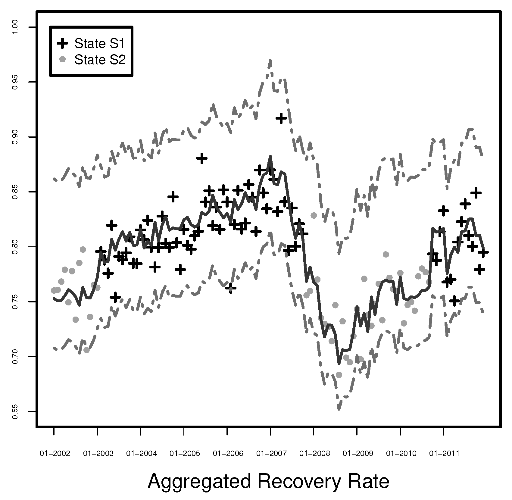
We have also considered beta, logit, probit, and log transformation of the ARR in the framework of linear regression as well as beta regression for the ARR. The linear regression model with a logarithmized response variable fits the ARR best and is extended in two directions. The first extension is built by adding interactions to the linear regression model. The second extension is a combination of the linear regression and a Markov switching model with two states, which can be interpreted as crisis and prosperity times. The reduced Markov switching model explains over 75 % of the variability of the aggregated recovery rates and outperforms the model with interactions. In prosperity times, the variables EURIBOR:3M, Unemployment, STOXX 50, and GGDP Europe are significant (at 5% or 1% level) drivers of the aggregated recovery rate at least while PRODUCTION (at level 10%) and GGDP (at 5% level) are significant indicators in crises times. Our out-of-sample comparison of the considered models shows the superiority of the Markov switching model in general and a good potential of the linear model with intersections.
Overall, the final model we propose uses a dynamic factor model with mixed frequency data to forecast the monthly GGDP, an optimal time shift in the variables, and a Markov switching model. The forecasted ARR could be used as an explanatory variable to model individual recovery rates. We expect that the modeling framework of Min et al. (2020); Sopitpongstorn et al. (2021) as well as Ye and Bellotti (2019) could gain more prediction power by considering the predicted ARR as an additional explanatory variable. The limitation of the proposed methodology is that the state of the Markov switching model is not known. For applications, this state should be predicted similarly to Hauptmann et al. (2014). Much empirical research on individual recovery rates using GDP or its interpolation, see, e.g., Calabrese (2014) and Gambetti et al. (2019), could be reconsidered by employing monthly extracted signals from GDP. Finally, the approach of Fermanian (2020) shows a great potential of copulas for describing the dependence structure of recovery rates and macroeconomic variables. This all is a topic of future research.

Author Contributions

Conceptualization, all authors; software, S.H., A.M., J.W.; validation, A.M., J.W.; formal analysis, all authors; investigation, all authors; resources, all authors; writing—original draft preparation, all authors; writing—all authors; visualization, A.M., J.W.; supervision, R.Z.; project administration, R.Z. All authors have read and agreed to the published version of the manuscript.

Funding

This research received no external funding.

Institutional Review Board Statement

Not applicable.

Informed Consent Statement

Not applicable.

Data Availability Statement

Aggregated recovery rate is not publicly available since it is computed using the database of Global Credit Data. Panel data is publicly available. The respective sources are stated in Appendix A in detail.

Acknowledgments

The authors would like to thank Global Credit Data for granting access to their database. They would also like to thank Nina Brumma for her helpful comments. Finally, the authors are grateful to the unknown referees for their constructive and helpful comments. This work was supported by the German Research Foundation (DFG) and the Technical University of Munich within the TUM Open Access Publishing Fund.

Conflicts of Interest

The authors declare no conflict of interest.

Appendix A. Data for GGDP Estimation

In this appendix, all variables for estimation of GGDP in Europe and GGDP in the USA are listed.

Appendix A.1. Data for European GGDP Estimation

Most of the variables are average values of 19 European countries: Austria, Belgium, Cyprus, Estonia, Finland, France, Germany, Greece, Ireland, Italy, Latvia, Lithuania, Luxembourg, Malta, Netherlands, Portugal, Slovakia, Slovenia, and Spain. The data is almost entirely taken from the website of the European central bank (http://sdw.ecb.europa.eu/ accessed on 31 March 2017 ). Only the VSTOXX volatility index observations are taken from a different source (https://www.investing.com/indices accessed on 5 April 2017).
Variable  Log   Diff   Monthly   Quarterly 
Industrial production total manufacturingxxx
Industrial production excluding constructionxxx
Industrial production intermediate goodsxxx
Industrial production capital goodsxxx
Industrial production energyxxx
Industrial production durable goodsxxx
Industrial production non-durable goodsxxx
Industrial production constructionxxx
New orders from domestic economyxxx
New orders—capital goodsxxx
New orders—manufacturingxxx
Inflation xx
EURIBOR—1-month rate xx
EURIBOR—3-months rate xx
10 years governmental bond yield xx
5 years governmental bond yield xx
Dow Jones Euro STOXX 50xxx
VSTOXX volatility indexxxx
exchange rate USD/Euro xx
GDPxx x
Private consumptionxx x
Gross Fixed Capital Formationxx x
Exportxx x
Importxx x
Gross value added x x
Gross value added—trade, transport, accomodation, food services x x
Property incomexx x
Entrepreneurial income—non-financial corporationsxx x
Entrepreneurial income—financial corporations GDPxx x

Appendix A.2. Data for US GGDP Estimation

The entire data used for derivation of US GGDP consists of 34 variables and is available at the webpage of the Research Division of the Federal Reserve Bank of St. Louis (https://fred.stlouisfed.org/ accessed on 27 March 2017).
Variable  Log   Diff   Monthly   Quarterly 
10-Years Aaa Corporate Bond Yieldxxx
10-Years Baa Corporate Bond Yieldxxx
New Orders: Consumer Nondurable Goods Industriesxxx
New Orders: All Manufacturing Industries Excluding Defensexxx
New Orders: Nondefense Capital Goods Industriesxxx
New Orders for Capital Goods Industriesxxx
New Orders: Durable Goodsxxx
Exchange rate USD/Euro xx
1-Year Treasury Constant Maturity Rate xx
10-Year Treasury Constant Maturity Rate xx
2-Year Treasury Constant Maturity Rate xx
3-Year Treasury Constant Maturity Rate xx
Industrial Production Index xx
Industrial Production: Consumer energy products xx
Industrial Production: Non-energy materials xx
Industrial Production: Construction supplies xx
Industrial Production: Consumer Goods xx
Industrial Production: Durable Consumer Goods xx
Industrial Production: Manufacturing (NAICS) xx
Industrial Production: Manufacturing (SIC) xx
Industrial Production: Nondurable Consumer Goods xx
3-Month Rates: Certificates of Deposit xx
Interbank Rate for the United States xx
Personal Consumption Expendituresxxx
Total Share Prices for All Shares for the United States xx
GDPxx x
Gross value added (IMA)xx x
Real Exports of Goods and Servicesxx x
Real Government Consumption Expenditures and Gross Investmentxx x
Real imports of goods and servicesxx x
Employed full time: Median usual weekly real earningsxx x
Nonfinancial noncorporate business; gross value added, Flowxx x
Gross Fixed Capital Formation in United Statesxx x

References

  1. Altman, Edward, and Vellore M. Kishore. 1996. Almost everything you wanted to know about recoveries on defaulted bonds. Financial Analysts Journal 52: 57–64. [Google Scholar] [CrossRef] [Green Version]
  2. Altman, Edward, Andrea Resti, and Andrea Sironi. 2001. Analyzing and Explaining Default Recovery Rates. ISDA Report. New York: ISDA. [Google Scholar]
  3. Amiram, Dan, and Edward L. Owens. 2021. Accounting-based expected loss given default and debt contract design. SSRN eLibrary. Available online: https://papers.ssrn.com/sol3/papers.cfm?abstract_id=1903721 (accessed on 9 August 2021).
  4. Asarnow, Elliot, and David Edwards. 1995. Measuring loss on defaulted bank loans: A 24-year study. The Journal of Commercial Lending 77: 11–23. [Google Scholar]
  5. Banbura, Marta, and Michele Modugno. 2014. Maximum likelihood estimation of factor models on data sets with arbitrary pattern of missing data. Journal of Applied Econometrics 29: 133–60. [Google Scholar] [CrossRef] [Green Version]
  6. Basel Committee on Banking Supervision. 2004. International Convergence of Capital Measurement and Capital Standards. Technical Report. Basel: Bank for International Settlement. [Google Scholar]
  7. Bastos, Joao A. 2010. Predicting Bank Loan Recovery Rates with Neural Networks. CEMAPRE Working Papers. Lisboa: CEMAPRE. [Google Scholar]
  8. Baum, Leonard E., Ted Petrie, George Soules, and Norman Weiss. 1970. A maximization technique occurring in the statistical analysis of probabilistic functions of Markov chains. The Annals of Mathematical Statistics 41: 164–71. [Google Scholar] [CrossRef]
  9. Bellotti, Anthony, Damiano Brigo, Paolo Gambetti, and Frédéric Vrins. 2021. Forecasting recovery rates on non-performing loans with machine learning. International Journal of Forecasting 37: 428–44. [Google Scholar] [CrossRef]
  10. Bellotti, Tony, and Jonathan Crook. 2012. Loss given default models incorporating macroeconomic variables for credit cards. International Journal of Forecasting 28: 171–82. [Google Scholar] [CrossRef] [Green Version]
  11. Brumma, Nina, Konrad Urlichs, and Wolfgang M. Schmidt. 2014. Modeling downturn LGD in a Basel framework. SSRN eLibrary. Available online: https://papers.ssrn.com/sol3/papers.cfm?abstract_id=2393351 (accessed on 10 October 2020).
  12. Calabrese, Raffaella. 2012. Estimating Bank Loans Loss Given Default by Generalized Additive Models. UCD Geary Institute Discussion Paper Series WP2012; Dublin: UCD Geary Institute. [Google Scholar]
  13. Calabrese, Raffaella. 2014. Predicting bank loan recovery rates with a mixed continuous-discrete model. Applied Stochastic Models in Business and Industry 30: 99–114. [Google Scholar] [CrossRef] [Green Version]
  14. Candian, Giacomo, and Mikhail Dmitriev. 2020. Default recovery rates and aggregate fluctuations. Journal of Economic Dynamics and Control 121: 104011. [Google Scholar] [CrossRef]
  15. Carey, Mark, and Michael Gordy. 2004. Measuring Systematic Risk in Recoveries on Defaulted Debt I: Firm-Level Ultimate LGDs; Cfr conference papers, Federal Deposit Insurance Corporation—Center for Financial Research. Washington, DC: Federal Reserve Board.
  16. Carrizosa, Richard, and Stephen G. Ryan. 2013. Conservatism, covenants, and recovery rates. SSRN eLibrary. Available online: https://papers.ssrn.com/sol3/papers.cfm?abstract_id=2197513 (accessed on 10 October 2020).
  17. Carty, Lea V., David T. Hamilton, and Adam Moss. 1999. Bankrupt bank loan recoveries. The Journal of Lending & Credit Risk Management 82: 20–26. [Google Scholar]
  18. Carty, Lea V., and Dana Lieberman. 1996. Corporate Bond Defaults and Default Rates 1938–1995. New York: Moody’s Investors Service Global Credit Research. [Google Scholar]
  19. Covitz, Daniel, and Song Han. 2004. An Empirical Analysis of Bond Recovery Rates: Exploring a Structural View of Default; Washington, DC: Board of Governors of the Federal Reserve System (U.S.).
  20. Defend, Monika, Alesey Min, Lorenzo Portelli, Franz Ramsauer, Francesco Sandrini, and Rudi Zagst. 2021. Quantifying drivers of forecasted returns using approximate dynamic factor models for mixed-frequency panel data. Forecasting 3: 56–90. [Google Scholar] [CrossRef]
  21. Dempster, Arthur P., Nan M. Laird, and Donald B. Rubin. 1977. Maximum likelihood from incomplete data via the EM algorithm. Journal of the Royal Statistical Society. Series B (Methological) 39: 1–38. [Google Scholar]
  22. Dermine, Jean, and C. Neto De Carvalho. 2006. Bank loan losses-given-default: A case study. Journal of Banking & Finance 30: 1219–43. [Google Scholar]
  23. Donovan, John, Richard M. Frankel, and Martin Xiumin. 2015. Accounting conservatism and creditor recovery rate. The Accounting Review 90: 2267–303. [Google Scholar] [CrossRef]
  24. Doz, Catherine, Domenico Giannone, and Lucrezia Reichlin. 2011. A two-step estimator for large approximate dynamic factor models based on Kalman filtering. Journal of Econometrics 164: 188–205. [Google Scholar] [CrossRef] [Green Version]
  25. Draper, Norman R., and Harry Smith. 1998. Applied Regression Analysis, 3rd ed. Wiley Series in Probability and Statistics; Hoboken: Wiley. [Google Scholar]
  26. Eales, Robert, and Edmund Bosworth. 1998. Severity of loss in the event of default in small business and larger consumer loans. Journal of Lending and Credit Risk Management 80: 58–65. [Google Scholar]
  27. EBA/GL/2016/07. 2016. Guidelines on the Application of the Definition of Default under Article 178 of Regulation (EU) No 575/2013. Available online: https://www.eba.europa.eu/documents/10180/1597103/Final+Report+on+Guidelines+on+default+definition+%28EBA-GL-2016-07%29.pdf/004d3356-a9dc-49d1-aab1-3591f4d42cbb (accessed on 15 March 2018).
  28. EBA/GL/2017/16. 2017. Guidelines on PD Estimation, LGD Estimation and the Treatment of Defaulted Exposures. Available online: https://www.eba.europa.eu/documents/10180/2033363/Guidelines+on+PD+and+LGD+estimation+%28EBA-GL-2017-16%29.pdf/6b062012-45d6-4655-af04-801d26493ed0 (accessed on 15 March 2018).
  29. Felsovalyi, Akos, and Lew Hurt. 1998. Measuring loss on Latin American defaulted bank loans: A 27-year study of 27 countries. Journal of Lending & Credit Risk Management 81: 41–46. [Google Scholar]
  30. Fermanian, Jean-David. 2020. On the dependence between default risk and recovery rates in structural models. Annals of Economics and Statistics, 45–82. [Google Scholar] [CrossRef]
  31. Frye, Jon. 2000. Depressing recoveries. Risk-London-Risk Magazine Limited 13: 106–11. [Google Scholar]
  32. Gambetti, Paolo, Geneviève Gauthier, and Frédéric Vrins. 2019. Recovery rates: Uncertainty certainly matters. Journal of Banking & Finance 106: 371–83. [Google Scholar]
  33. Grunert, Jens. 2010. Verwertungserlöse von Kreditsicherheiten: Eine empirische Analyse notleidender Unternehmenskredite. Zeitschrift für Betriebswirtschaft 80: 1305–23. [Google Scholar] [CrossRef]
  34. Grunert, Jens, and Martin Weber. 2005. Recovery Rates of Bank Loans: Empirical Evidence for Germany. Available online: http://ub-madoc.bib.uni-mannheim.de/1073 (accessed on 10 October 2020).
  35. Hauptmann, Johannes, Anja Hoppenkamps, Aleksey Min, and Rudi Zagst. 2014. Forecasting market turbulence using regime-switching models. Financial Markets and Portfolio Management 28: 139–64. [Google Scholar] [CrossRef]
  36. Hu, Yen-Ting, and William Perraudin. 2002. The Dependence of Recovery Rates and Defaults. Working paper. London: Birkbeck College. [Google Scholar]
  37. Ingermann, Peter-Hendrik, Frederik Hesse, Christian Belogrey, and Andreas Pfingsten. 2016. The recovery rate for retail and commercial customers in Germany: A look at collateral and its adjusted market values. Business Research 9: 179–228. [Google Scholar] [CrossRef] [Green Version]
  38. Jankowitsch, Rainer, Florian Nagler, and Marti G. Subrahmanyam. 2014. The determinants of recovery rates in the US corporate bond market. Journal of Financial Economics 114: 155–77. [Google Scholar] [CrossRef] [Green Version]
  39. Keijsers, Bart, Bart Diris, and Erik Kole. 2018. Cyclicality in losses on bank loans. Journal of Applied Econometrics 33: 533–52. [Google Scholar] [CrossRef] [Green Version]
  40. Khieu, Hinh D., Donald J. Mullineaux, and Ha-Chin Yi. 2012. The determinants of bank loan recovery rates. Journal of Banking & Finance 36: 923–33. [Google Scholar]
  41. Krüger, Steffen, and Daniel Rösch. 2017. Downturn LGD modeling using quantile regression. Journal of Banking & Finance 79: 42–56. [Google Scholar]
  42. Min, Aleksey, Matthias Scherer, Amelie Schischke, and Rudi Zagst. 2020. Modeling recovery rates of small- and medium-sized entities in the US. Mathematics 8: 1856. [Google Scholar] [CrossRef]
  43. Nakata, Taisuke, and Christopher Tonetti. 2010. Kalman Filter and Kalman Smoother. Working Paper. Available online: https://christophertonetti.com/miscellany.html (accessed on 10 October 2020).
  44. Qi, Min, and Xinlei Zhao. 2011. Comparison of modeling methods for loss given default. Journal of Banking & Finance 35: 2842–55. [Google Scholar]
  45. Schuermann, Til. 2004. What do we know about loss given default? SSRN eLibrary. Available online: https://papers.ssrn.com/sol3/papers.cfm?abstract_id=525702 (accessed on 10 October 2020).
  46. Schumacher, Christian, and Breitung Jorg. 2008. Real-time forecasting of German GDP based on a large factor model with monthly and quarterly data. International Journal of Forecasting 24: 386–98. [Google Scholar] [CrossRef]
  47. Sopitpongstorn, Nithi, Param Silvapulle, Jiti Gao, and Jean-Pierre Fenech. 2021. Local logit regression for loan recovery rate. Journal of Banking & Finance 126: 106093. [Google Scholar]
  48. Tipping, Michael E., and Christopher M. Bishop. 1999. Probabilistic principal component analysis. Journal of the Royal Statistical Society: Series B (Statistical Methodology) 61: 611–22. [Google Scholar] [CrossRef]
  49. Viterbi, Andrew. 1967. Error bounds for convolutional codes and an asymptotically optimum decoding algorithm. IEEE Transactions on Information Theory 13: 260–69. [Google Scholar] [CrossRef] [Green Version]
  50. Wang, Hong, Catherine S. Forbes, Jean-Pierre Fenech, and John Vaz. 2020. The determinants of bank loan recovery rates in good times and bad–new evidence. Journal of Economic Behavior & Organization 177: 875–97. [Google Scholar]
  51. Ye, Hui, and Anthony Bellotti. 2019. Modelling recovery rates for non-performing loans. Risks 7: 19. [Google Scholar] [CrossRef] [Green Version]
Figure 1. Observed quarterly (grey pluses)and estimated monthly (black dotes) European GDDP.
Risks 10 00018 g001
Figure 2. Observed quarterly (grey pluses) and estimated monthly (black dotes) US GDDP.
Risks 10 00018 g002
Figure 3. Frequencies of recovery rates.
Risks 10 00018 g003
Figure 4. Average recovery rates computed for every percentile of S&P500 (top left), STOXX 50 (top right), GY (bottom left) and VSTOXX (bottom right).
Risks 10 00018 g004
Figure 5. S&P500 (top left) and STOXX 50 (top right) vs. aggregated recovery rates (bottom).
Risks 10 00018 g005
Figure 6. European GGDP (top left) and Unemployment (top right) vs. aggregated recovery rates (bottom).
Risks 10 00018 g006
Figure 7. Shifted S&P500 (top left) and STOXX 50 (top right) vs. recovery rate (bottom).
Risks 10 00018 g007
Figure 8. Shifted European GGDP (top left) and Unemployment (top right) vs. recovery rate (bottom).
Risks 10 00018 g008
Figure 9. Sensitivity of the logarithmized ARR on S&P500 and STOXX50.
Risks 10 00018 g009
Figure 10. Observed and predicted aggregated recovery rates.
Risks 10 00018 g010
Figure 11. Prediction error distribution with 5% and 95% quantiles (grey vertical lines) for the models with no time shifts (top left), 6.month time shift (top right), 12-month time shift (bottom left) and optimal time shifts (bottom right).
Risks 10 00018 g011
Figure 12. Monthly aggregated recovery rates with 99% prediction interval (grey dot-dash line) and the mean of the predictions (grey solid line) at the time of default for Model (6).
Risks 10 00018 g012
Figure 13. Monthly aggregated recovery rates with 99% prediction interval (grey dot-dash line) and the mean of the predictions (grey solid line) 3 and 6-months after default for Model (6).
Risks 10 00018 g013
Figure 14. Monthly aggregated recovery rates with 99% prediction interval (grey dot-dash line) and the mean of the predictions (grey solid line) 9 and 12 months after default using empirical distributions for Model (6).
Risks 10 00018 g014
Figure 15. Sensitivity of the logarithmized ARR on S&P500 (left) and STOXX50 (right).
Risks 10 00018 g015
Figure 16. Sensitivity of the logarithmized ARR on Unemployment (left) and GGDP Europe (right).
Risks 10 00018 g016
Figure 17. Sensitivity of the logarithmized ARR on a joint movement of S&P500 and STOXX50.
Risks 10 00018 g017
Figure 18. Monthly aggregated recovery rates with 99% prediction interval (grey dot-dash line) and the mean of the predictions (grey solid line) at the time of default for the reduced model with intersections.
Risks 10 00018 g018
Figure 19. States sequence of the Markov chain.
Risks 10 00018 g019
Figure 20. Monthly aggregated recovery rates with 99% prediction interval (grey dot-dash line) and the mean of the predictions (grey solid line) at the time of default for the reduced Markov switching model.
Risks 10 00018 g020
Figure 21. Out-of-sample prediction of the linear model (LM), the linear model with intersecations (LMwI) and the Markov switsching model (MSM) for static models (left) and the dynamic models (right). The observed ARR is displayed in the solid line.
Risks 10 00018 g021
Table 1. Basic statistics of recovery rates.
SimpleWeighted
Mean0.7860.746
St.dev0.2960.281
Median0.9510.878
25%–Quantile0.6640.556
75%–Quantile0.9890.978
Table 2. Fitted linear regression (4) with unshifted variables before and after model selection.
Full ModelAIC Model
VariableCoefficient (Standard Error)Coefficient (Standard Error)
(Intercept) 1.195 ** ( 0.386 ) 1.04 *** ( 0.126 )
EURIBOR:1M 0.101 *** ( 0.029 ) 0.088 *** ( 0.026 )
EURIBOR:3M 0.064 * ( 0.032 ) 0.061 ** ( 0.021 )
Inflation 0.023 * ( 0.009 ) 0.025 *** ( 0.007 )
Unemployment 0.005 ( 0.028 )
S&P500 1.140 · 10 4 ( 1.001 · 10 4 )
STOXX 50 2.110 · 10 5 ( 2.435 · 10 5 )
GY 0.031 ** ( 0.010 ) 0.020 * ( 0.008 )
VSTOXX 0.001 ( 0.001 )
Production 0.010 *** ( 0.003 ) 0.008 *** ( 0.001 )
GGDP Europe 0.662 ( 0.526 )
GGDP USA 7.185 * ( 3.221 ) 10.216 *** ( 2.256 )
R 2 0.5280.497
Adj. R 2 0.4790.470
Num. obs.120120
RMSE0.0400.040
*** p < 0.001, ** p < 0.01, * p < 0.05.
Table 3. Correlations between the ARR and explanatory variables before and after optimal time shifts.
Correlation Pre-ShiftShift in MonthsCorrelation Post-Shift
VSTOXX 0.522 0 0.522
GY 0.013 12 0.316
GGDP USA 0.515 0 0.515
GGDP Europe 0.357 2 0.471
Production 0.324 10 0.747
EURIBOR: 1M 0.043 18 0.604
EURIBOR: 3M 0.039 18 0.619
Inflation 0.018 12 0.564
Unemployment 0.015 18 0.456
SP 500 0.470 6 0.712
STOXX 50 0.367 6 0.635
Table 4. Fitted linear regression models (5) and (6) with shifted variables.
Full ModelAIC Model
VariableCoefficient (Standard Error)Coefficient (Standard Error)
(Intercept) 0.239 ( 0.216 ) 0.085 ( 0.057 )
EURIBOR: 1M 0.028 ( 0.020 )
EURIBOR: 3M 0.038 ( 0.022 )
Inflation 0.010 ( 0.007 )
Unemployment 0.017 ( 0.013 ) 0.034 *** ( 0.005 )
S&P500 2.505 · 10 4 *** ( 5.749 · 10 5 ) 3.337 · 10 4 *** ( 3.570 · 10 5 )
STOXX 50 5.977 · 10 5 ** ( 2.167 · 10 5 ) 7.542 · 10 5 *** ( 1.449 · 10 5 )
GY 0.004 ( 0.005 )
VSTOXX 3.969 · 10 4 ( 4.089 · 10 4 )
Production 2.985 · 10 4 ( 0.002 )
GGDP Europe 0.863 * ( 0.386 ) 0.924 ** ( 0.339 )
GGDP USA 2.006 ( 2.694 )
R 2 0.7110.688
Adj. R 2 0.6820.677
Num. obs.120120
RMSE0.0310.032
*** p < 0.001, ** p < 0.01, * p < 0.05.
Table 5. R a d j 2 for linear models with different time shifts.
Adjusted R adj 2
0-Shift 0.479
6 m-Shift 0.630
12 m-Shift 0.599
Optimal Shift 0.682
Table 6. Fitted linear regression model (7) with interactions before and after model selection.
Full ModelAIC Model
VariableCoefficient (Standard Error)Coefficient (Standard Error)
(Intercept) 1.040 ** ( 0.394 ) 0.503 ( 0.257 )
Unemployment 0.126 *** ( 0.033 ) 0.094 *** ( 0.028 )
S&P500 0.001 ** ( 3.639 · 10 4 ) 0.001 * ( 3.169 · 10 4 )
STOXX 50 3.257 · 10 5 ( 1.020 · 10 4 ) 1.578 · 10 4 * ( 7.088 · 10 5 )
GGDP Europe 0.633 ( 7.773 ) 0.317 ( 1.662 )
Unemployment x S&P500 1.202 · 10 4 *** ( 3.124 · 10 5 ) 1.030 · 10 4 *** ( 3.018 · 10 5 )
Unemployment x STOXX 50 1.793 · 10 5 * ( 6.871 · 10 6 ) 2.121 · 10 5 ** ( 6.471 · 10 6 )
Unemployment x GGDP Europe 0.096 ( 0.64 )
S&P500 x STOXX 50 7.157 · 10 8 ( 3.923 · 10 8 )
S&P500 x GGDP Europe 0.005 ( 0.003 ) 0.006 * ( 0.003 )
STOXX 50 x GGDP Europe 0.002 ( 0.002 ) 0.002 * ( 0.001 )
R 2 0.7340.724
Adj. R 2 0.7090.704
Num. obs.120120
RMSE0.0300.030
*** p < 0.001, ** p < 0.01, * p < 0.05.
Table 7. Estimated parameters of the Markov switching model.
State S1State S2
δ 01
π · 1 0.9840.016
π · 2 0.0450.955
μ −0.206−0.287
σ 0.0380.039
Table 8. Fitted regression model (8) with 2 Markov states before stepwise model selection.
State S1State S2
VariableCoefficient (Standard Error)Coefficient (Standard Error)
(Intercept) 2.692 · 10 4 ( 0.388 ) 0.1023 ( 0.503 )
EURIBOR: 1M 0.009 ( 0.029 ) 0.074 ( 0.074 )
EURIBOR: 3M 0.027 ( 0.033 ) 0.020 ( 0.085 )
Inflation 0.001 ( 0.010 ) 0.010 ( 0.018 )
Unemployment 0.022 ( 0.024 ) 0.034 ( 0.039 )
S&P 500 3.646 · 10 5 ( 1.362 · 10 4 ) 1.867 · 10 4 ( 1.286 · 10 4 )
STOXX 50 6.912 · 10 5 ( 4.771 · 10 5 ) 8.218 · 10 5 ( 4.798 · 10 5 )
GY 0.007 ( 0.006 ) 0.030 ( 0.025 )
VSTOXX 1.428 · 10 4 ( 0.001 ) 1.018 · 10 4 ( 0.001 )
Production 0.006 ( 0.004 ) 0.004 ( 0.003 )
GGDP Europe 1.174 ( 0.594 ) 1.183 * ( 0.579 )
GGDP USA 2.776 ( 7.230 ) 5.520 ( 5.614 )
R 2 0.7708
Adj. R 2 0.7159
Num. obs.120
*** p < 0.001, ** p < 0.01, * p < 0.05.
Table 9. Fitted regression models (8) with 2 Markov states after stepwise model selection.
State S1State S2
VariableCoefficient (Standard Error)Coefficient (Standard Error)
(Intercept) 0.124 ( 0.247 ) 0.433 ( 0.251 )
EURIBOR:3M 0.021 * ( 0.009 )
Unemployment 0.027 ** ( 0.008 ) 0.020 ( 0.014 )
S&P500 1.446 · 10 4 ( 9.477 · 10 5 )
STOXX 50 7.359 · 10 5 ** ( 2.670 · 10 5 ) 6.048 · 10 5 ( 3.127 · 10 5 )
GY 0.008 ( 0.005 ) 0.019 ( 0.014 )
Production 5.568 · 10 3 ( 3.223 · 10 3 ) 4.223 · 10 3 ( 2.177 · 10 3 )
GGDP Europe 1.116 * ( 0.530 ) 1.3 * ( 0.487 )
R 2 0.759
Adj. R 2 0.737
Num. obs.120
*** p < 0.001, ** p < 0.01, * p < 0.05.
Publisher’s Note: MDPI stays neutral with regard to jurisdictional claims in published maps and institutional affiliations.

