
Spatial-Temporal Evolution and Risk Assessment of Land Finance: Evidence from China

1
Department of Land Resources Management, China Institute of Land and Urban Governance, Zhejiang Gongshang University, 18 Xuezheng St., Xiasha University Town, Hangzhou 310018, China
2
Department of Transportation, Logistics and Finance, North Dakota State University, Fargo, ND 58108, USA
3
Department of Agricultural and Biosystems Engineering, North Dakota State University, Fargo, ND 58108, USA
4
College of Land Science and Technology, China Agricultural University, Beijing 100193, China
*
Author to whom correspondence should be addressed.
Risks 2022, 10(10), 196; https://doi.org/10.3390/risks10100196
Submission received: 19 August 2022
/
Revised: 27 September 2022
/
Accepted: 6 October 2022
/
Published: 12 October 2022
Abstract
:Land finance is a special land financing mode in China under the nationalization of urban land since 1954. The policy authorizes local governments to collect fiscal revenue from land grant premiums and land taxes. As China is experiencing the social and economic transformation, heavily replying on land finance starts causing financial sustainable problems. Based on the spatial panel data of 30 provinces in China in the last two decades, we analyzed the spatial-temporal evolution of land finance. We found that the spatial variation of land finance declined during the period of study and decreased from east to west. The results revealed that land finance had significant positive spatial autocorrelation and robust spatial clustering characteristics. In addition, the spatial distribution of land finance was consistent with the population-based Hu Line. We also assessed land finance risks via a four-dimensional risk matrix through spatial panel regression (SPR). The spatial spillover effects suggested that there is inter-provincial imitation and collaboration but no competition. Our forecast indicates that most provinces will be at a relatively low risk level in the next decade except some southwest provinces. Based on the findings, we highlight the policy implications to mitigate risks and maintain sustainable land finance.
1. Introduction
Since China’s economic reform in 1978, especially after the 1990s, the lack of finance revenue and high cost of urban construction have led local governments to rely more on the strategy of “land for capital” to develop the economy (Ye and Wang 2013; Huang and Chan 2018; Xu 2019; Ma and Mu 2020). As a unique economic phenomenon in China, land finance has become an important way for local governments to obtain extra revenue to fill budget deficits in the past 40 years (Liu and Lin 2014; Tang et al. 2019). Land finance in China has played a significant role in promoting local social and economic development and urbanization (Geng et al. 2018), enhancing the disposable capacity of local revenue (Fu and Lin 2013), and arousing the enthusiasm of local governments to participate in resource reallocations (Gao et al. 2014).
However, land finance has been proved as a double-edged sword. On one hand, land finance creates huge financial revenue for local governments, provides financial support to urban construction and development, and accelerates the local urbanization development (Geng et al. 2018; Tang et al. 2019; Zhong et al. 2019). On the other hand, land finance is not a sustainable financial system (Chen and Hu 2015). It may distort the optimal allocation of economic resources and break the social equality of income distribution. As China is experiencing the social and economic transformation, heavily replying on land finance has been causing financial sustainable problems.
Land finance in China has received considerable attention in academic studies. Existing studies mainly focused on examining driving factors of land finance (Ye and Wang 2013; Wang and Ye 2016; Lu et al. 2019), investigating the relationship between land finance and some political, social, and economic characteristics (China’s economic fluctuation—Tao et al. 2010; urbanization development—He et al. 2016; real estate prices—Pan et al. 2015; land use policy violation—Wang and Scott 2013; local government debt—Tsui 2011; land expropriation and compensation—Hui et al. 2013), and assessing social welfare effect of land finance (Han et al. 2019). However, most of the studies aim at certain types of districts or areas. The literature lacks studies that explore land finance at national-provincial level and depict a country-wide situation of land finance that central and local governments can refer to when adjusting land policies. In our study, we proposed a measure of land finance that considers the tax revenue, the non-tax revenue, and the revenue from the mortgage and financing of land. Based on the most recent data, we conducted an analysis to jointly inspect the spatial and temporal evolution of land finance in China over the last two decades and provide updates on provincial variations and trends of land finance. In addition, our paper discusses the key risk factors for land finance across provinces based on sub-zone and sub-stage models through spatial panel regression (SPR). The model also incorporates spatial factors to capture the spatial spillover effects on land finance. We found that land finance across provinces possess learning and collaborative relationships.
China is now experiencing a crucial period of economic and social transformation. With the advancement of the new-type urbanization strategy and rapid population growth (Yang 2013), the conflicts between limited land resources and unlimited urbanization will remain or even grow in severity in the future (He et al. 2006; Mullan et al. 2011; Lian and Lejano 2014; Cai et al. 2020). Risks associated with land finance have led to unsustainable developments of the social economy. Moreover, heavily relying on land finance may lead to more hidden risks. Land finance risks have gradually attracted social attention and become an important research field recently. However, most studies in this area either involve only qualitative discussions or focus only on regional issues. Based on Zhang et al. (2020), we propose a composite four-dimensional land finance risk assessment matrix that considers economic risk, social risk, legal risk, and ecological risk. Furthermore, we use a grey forecasting model GM(1,1) to detect potential high land finance risks and send early warnings to the policyholders at the first opportunity.
In sum, based on the panel data from 30 provinces of China in the last two decades, we contribute to the literature by (1) exploring spatial-temporal evolution and pattern of land finance, (2) constructing an index system to assess land finance risks and make early warnings, (3) identifying the key risk factors of land finance, (4) investigating the spatial spillover effects of land finance, (5) predicting the land finance risk in the next decade, and (6) presenting political implications of mitigating land finance risks to policymakers and local governments.
The rest of the paper is organized as follows: Section 2 provides an overview of land finance in China. Section 3 introduces the methodologies and data. We first define a comprehensive measure of land finance. Then, we explain our research tools, including the average growth index (AGI), the Moran’s I, the Getis-Ord G, the four-dimensional land finance risk matrix, and the grey forecasting model. The data and software are described in Section 3.7. We present our findings from the spatial-temporal empirical analyses in Section 4. Section 5 offers a discussion of policy implications. We conclude the paper in Section 6.
2. An Overview of Land Finance in China
In 1994, China carried out a financial decentralization reform (Jia et al. 2014). The added-value tax was changed to a shared tax between the central government and local governments. Local governments were required to pay the central government 75 percent of the added-value tax (Wang and Ye 2016). The central government remained part of financial rights and obtained better tax sources (Fu 2015). Since the reform increased the central government’s revenue and capacity to pay (Figure 1a), the central government was able to support the socio-economic development of poor and undeveloped areas through transferred payments (Pan et al. 2017). This strengthened the central government’s ability to control local development.
However, local governments still need to bear huge costs and fees of urban construction, including constructive fund, administrative expenditures, project supporting fund, non-public welfare expenditures, social security expenditures, and enterprise subsidies (Guo 2009; Wang et al. 2011; Wu et al. 2015; Hu and Qian 2017). As the expenditure responsibility of local governments kept increasing in the last four decades (Figure 1b), the lack of stable financial revenue for local governments after the transfer of financial power broke the balance of revenue and expenditures. Under this background, land transfer and land transactions have become an important channel for local governments to raise capital to resume the balance between local revenue and expenditures. Although some scholars questioned the widely accepted conventional theory of tax-sharing reform (Xu 2019), most studies agreed that the tax-sharing system was the main reason for land finance.
The China official performance evaluation system also promotes land finance. On one hand, the GDP-based official performance evaluation system has indirectly accelerated the development of land finance policies (Meng et al. 2019). Local officials need to keep raising GDP and handing over revenue to the central government in order to show their personal achievements and gain rapid career advancement (Shi et al. 2018). As local officials struggle to find new sources of revenue, land finance is a major source of revenue. By attracting investments and enlarging the scale of land development, local governments can not only promote economic development but also show their administrative achievements (Smith 2013; Li et al. 2016). On the other hand, the current tenure system of local officials in China has encouraged officials to make local development decisions based on personal promotion, whereas adverse consequences will be borne by their successors (Chen et al. 2017). To obtain land transfer fees, officials may sacrifice farmers’ interests to lower the land price, leading to the abuse of public power for private gains.
Traditional urbanization and socio-economic development are also important contributors to land finance in China. To speed up urbanization and expand the investment scale, a large amount of capital is needed to invest in infrastructure construction (Huang et al. 2015). In recent years, urban expansion and increased investment have led to a boom in land markets. The increased tax revenue significantly contributed to the local economy (Zhang 2000). Specifically, the real estate tax and construction tax accounted for around one-third of the whole local tax revenue in the developed regions of China (Han and Kung 2015). The fees and taxes from land transfer had brought financial benefits to local governments. However, under the current people-oriented new-type urbanization strategy, the development model of traditional land-oriented urbanization (land for capital) no longer conforms to the future development of China.
After China’s 2015 supply-side structural reform, the social and economic development is facing a series of new issues. The slowdown of economic growth, the sharp decline of fixed asset investment (e.g., real estate investment), the changes of land use structure, the downward trend of land price, the shrinking land area for sale, and the lack of land market demand, have led to an apparent decline in national land transaction revenue. These changes have forced the central government to reconsider land finance supervision. It is urgent to mitigate the negative impacts of land finance through proper regulation and risk management (Tao et al. 2010; Ye and Wang 2013; Jia et al. 2014).
3. Methods and Data
3.1. Measurement of Land Finance
Land finance refers to a strategy that relies on land grant premiums and land taxes as the major fiscal revenue for local governments (Wu et al. 2015; Wang and Ye 2016). Some cities adopted the unsaturated land supply and sold such land at prices as high as possible (Du and Peiser 2014; Qin et al. 2016). In recent years, land finance has evolved from a simple land trading phenomenon into a systematic land financing pattern (Li and Peng 2018).
There is not a common definition of land finance in China. Most scholars agree that land finance satisfies the following two basic characteristics: (1) the financial revenue of local governments relies heavily on land-related revenue (Jia et al. 2014; Pan et al. 2017; Tang et al. 2019); and (2) the land transfer fees account for a great proportion of the financial revenue of land.
Different from Wang and Ye (2016)’s study that limits the discussion of land finance to the local non-tax revenue, our measure of land finance considers most sources of revenue generated from land finance, which consists of three parts: (i) non-tax revenue of land, (ii) tax revenue of land, and (iii) mortgage and financing revenue of land. Specifically, land finance is computed as follows:
Land finance (LF) = land transfer fee + urban land use tax
+ land value added tax + farmland occupation tax + deed tax
+ real estate related tax.
+ land value added tax + farmland occupation tax + deed tax
+ real estate related tax.
Figure 2 demonstrates the composition of land finance, where the bold components are included in the calculation of land finance (see Equation (1)). The non-tax revenue of land includes land rent, land transfer fee, and other land-related fee income. The land transfer fee refers to the transaction fees collected from the land management departments of all levels of government when the land-use right is transferred to the land user. The transfer fee also includes renewal fees since when a land use period expires, the land user needs to renew the land-use right and pay the renewal land transfer price to the land management department. The tax revenue of land includes both direct and indirect tax revenue. The direct land revenue includes urban land use tax, housing property tax, land value-added tax, farmland land occupation tax, and deed tax. The urban land use tax refers to a tax levied by the state on the units and individuals who use land within the cities, counties, towns, and industrial and mining areas. Here, the land value-added tax is a tax levied on the value-added obtained from transferring state-owned land-use rights of above-ground buildings and their attachments. The farmland land occupation tax is a tax levied on units and individuals who occupy cultivated land to build houses or engage in other non-agricultural construction. And the deed tax is a one-time tax levied on the new owner (the property right heir) as a certain percentage of the production price when the property right of the real estate (land, house) changes. The indirect tax revenue refers to tax income indirectly related to land, including real estate-related tax and construction industry-related tax. The amount of such indirect tax is determined based on the taxable residual of the house or the rental income. Furthermore, land finance includes the mortgage and financing revenue of land.
3.2. Average Growth Index
In this study, following Jin and Lu (2009), we use the average growth index (AGI) to measure the change tendency of land finance during the investigated period, which can be expressed as follows:
where and are the values of land finance in years and , respectively.
3.3. Global Moran’s I and Getis-Ord G
Global Moran’s I and Getis-Ord G are two common tools to depict spatial characteristics of variables. Mainly used to explore the overall spatial autocorrelation of variables, Moran’s I is defined as (Anselin 1995):
where and are the values of land finance at the spatial unit and , respectively; ; is the total number of assessment units, and is the average value of . Here, is the spatial weight defined by the adjacency of the eight nearest units (Queen’s contiguity). When and are adjacent, otherwise . The value of Moran’s I is between −1 (indicating perfect dispersion) and 1 (indicating perfect aggregation). The Z-score for Moran’s I, , is computed as:
where
and
A positive means data are spatially clustered, while a negative indicates that data are clustered in a competitive way. Statistically, when is large enough and the corresponding p-value is lower than the desired significance level, we reject the null hypothesis and claim that “there is spatial clustering of the values associated with the geographic features”.
Getis-Ord G is primarily used to reveal the clustering characteristics of land finance and the local spatial aggregation. The G values range from 0 to 1, and is defined as (Getis and Ord 1992):
The Z-score for G is computed as:
where
and
When , the spatial pattern is a high-high cluster or low-low cluster; when , the spatial pattern is a high-low or low-high cluster; when , the spatial pattern is perfectly randomly distributed with no association.
3.4. Composite Risk Index Model of Land Finance Risk
Our composite risk assessment process follows the four steps described below.
- Step 1. Constructing the assessment index system of land finance risk
Based on risk sources and effects, we assessed land finance risks with a diversified assessment index system. Specifically, we proposed a four-dimensional matrix that jointly consider economic risk, social risk, legal risk, and ecological risk to assess land finance risks (Figure 3). First, economic risk associated with the abuse of land finance and the real estate bubbles in the overheated markets. Second, social risk caused by the increase in housing prices and the deterioration of equality in the land market. Third, legal risk due to the crimes caused by interest conflicts in land expropriation. Fourth, ecological risk arose with the destruction of ecological land and the decrease of cultivated land during the adjustment of land uses.
Following the existing literature (Zheng et al. 2014; Zhou et al. 2019; Zhang et al. 2020), we developed a set of land finance assessment indicators based on the proposed risk assessment framework. We considered 15 risk variables in our four-dimensional framework, based on the objectiveness, scientific soundness, dynamics, practicability, maneuverability, and availability of the data. As existent literature reveals, social risk of land finance is related to the social anxiety caused by the ever-growing urban commercial housing price and the enlarging income gap between urban and rural populations. The social contradictions due to competitive needs between construction and cultivated land may also contribute to social risk. As such, we consider six relevant indicators, which are the urbanization rate, increase of developed land, average housing price growth rate, the income disparity between urban and rural residents, degree of development of land markets, and cultivated land per capita. To assess economic risk, we considered a few tax and deficit/revenue related indicators that include the deficit ratio, macro tax burden, and the asset-liability ratio of real estate enterprises. In addition, we added the proportion of land finance scaled by local revenue to measure the dependence of the local government on land finance. The major legal risk results from land-associated illegal acts by local governments, therefore we included three related risk indicators, which are the number of land violation cases, the number of illegal land occupation cases, and the percentage of cultivated land in illegal occupation cases. Furthermore, we used two indicators, i.e., the percentage of cultivated land area and the cultivated land decrease rate to evaluate the ecological risk posed by land finance to the environment. In Table 1, we listed these variables and provide the variable descriptions. In the last column of Table 1, we presented our expected influences (positive vs. negative) of these factors on land finance.
- Step 2. Normalize the original data
Since the variables Z in Table 1 have different units and distributions, following Su et al. (2011), we normalized them to values between 0.1 and 0.9 (variables X) to facilitate arithmetic operation and comparative analyses1:
where is the normalized value of ; is the original value of the risk variable ( in unit ( in year t (; and and are the maximum value and minimum value of , respectively.
- Step 3. Calculate the weight of each risk factor
We then determined the weight of each risk factor following the analytic hierarchy process (AHP) (Saaty 1994) and the method of entropy (Shannon and Weaver 1949; Zhou et al. 2015). To figure out the AHP weights for the risk factors, we first constructed a pairwise comparison matrix based on the relative importance of the criterion versus ( as follows:
where and are the normalized weights of variables and , satisfying and . Please refer to the online Supplementary Materials I Table S1 for the pairwise comparison matrix of the fifteen ( proposed risk factors. Obviously and . We further assumed satisfies an eigenvalue equation:
where is the maximal eigenvalue of matrix . That means, the AHP weights are the components of the eigenvector by solving Equation (14).
To calculate the entropy weight, we first calculated the entropy value of the k-th risk factor as follows:
where and are the number of spatial units and years. Then the entropy weight of risk factor , , equals:
Therefore, the combined weight of risk factor , , is calculated as:
where is the weight of factor by AHP and is the entropy weight of factor .
- Step 4. Calculate the composite risk index
Once the risk factors and their weights are determined, the composite risk index (CRI) of land finance by centesimal system scoring can be calculated via a weighted linear model as follows:
where is the composite risk index in year for unit , is the normalized value of risk factor in unit in year and is the weight of risk factor .
3.5. Grey Forecasting Model GM(1,1)
The grey system theory proposed by Deng (1982) has been widely applied in risk assessment in multiple research areas, such as soil salinization (Zhou et al. 2013), meteorological disaster management (Gong and Forrest 2014), energy consumption (Yuan et al. 2016), and output prediction (Javed and Liu 2018). In this study, we used the grey forecasting GM(1,1) model to detect the early warnings of land finance risks at the provincial level. Furthermore, the predicted values of CRI are divided into 5 levels: non-warning (<20), light warning (20–40), moderate warning (40–60), severe warning (60–80), and very severe warning (>80).
In a basic GM(1,1) model (Deng 1982), we define , , and , where and . Then we have . The parameters and are the development coefficient and grey action quantity, respectively. The time responded functions of the GM(1,1) model are as follows:
where is the simulative value of and is the simulative value of .
The goodness of fit of the GM(1,1) model is judged based on the criteria presented in Table 2. More details for the extended form of the GM(1,1) model can be found in Deng (1982) and Zhou and He (2013).
3.6. The SPR Model
On one hand, there may be a two-way interaction between land finance and its risk factors in Table 1; on the other hand, risk factors may be correlated. Therefore, when there is a significant spatial autocorrelation among risk factors, we employed the spatial panel regression (SPR) model to assess the key risk factors for land finance. The advantages of the spatial panel regression model are three folds.
First, classical econometric models do not incorporate spatial weights, i.e., neighbor relations (Anselin 1995). Spatial panel regression models, instead, allow shocks on explanatory variables to be transmitted to all other “neighbors” within the spatial network (Foglia and Angelini 2019). If variables have spatial autocorrelation, the parameter setting and estimation of traditional regression models (e.g., the linear regression model based on ordinary least squares) may be biased, whereas the spatial panel regression model that considers both spatial effect and temporal effect can better reflect the influence of risk factors (explanatory variables) on land finance (dependent variable). Second, the spatial panel data contain a mass of information (Wang et al. 2016), which can better construct and test the close and complex linkages across different provinces. Third, the panel data can also increase the model’s degree of freedom, reduce the degree of multicollinearity between explanatory variables, and improve the estimation efficiency (Ye and Wang 2013).
According to Elhorst (2010) and Anselin et al. (2008), when both spatial effect and temporal effect are considered, the scalar equations of the spatial panel regression model can be expressed as follows:
where is the spatial autoregressive coefficient and is the spatial weight between units and . Here, indicates the spatial spillover effects (i.e., there is competition relationship of land finance between adjacent regions); means the spatial agglomeration effects (i.e., there is a cooperative relationship between adjacent regions). Since there are risk factors, the independent variable is a row vector of observations in spatial unit ( at time (. Additionally, is the regression coefficient vector, is the spatial autocorrelation error term, represents the spatial specific effect, and represents a temporal specific effect. Furthermore, if or is related to , the model considers fixed effect to address the spatial effect or the time effect; otherwise, the model is a random effect model. In Equation (22), is the spatial autocorrelation coefficient and is the random disturbance term.
3.7. Data and Software
We collected the panel data of 30 provinces2 in mainland China for the last two decades. Our data were collected from multiple China’s statistical yearbooks, including the China Land and Resources Statistical Yearbook, the China City Statistical Yearbook, the China Population and Employment Statistics Yearbook, and the China Real Estate Statistics Yearbook. The digital administrative boundary data were collected from the National Geomatics Center of China3. The principal sources of the China Land and Resources Statistical Yearbook were administered by the Ministry of Land and Resources before 2017; after that, the yearbook has been instead managed by the Ministry of Natural Resources4. Due to this institutional change, a few key variables of our study (e.g., land finances fees; risk factors , , and in Table 1) were no longer reported in the China Land and Resources Statistical Yearbook after 2017. In addition, there is a structural disconnection between the 2001–2016 and the post-2016 data. Therefore, we consider only the data for the period 2001–2016 in our spatial-temporal empirical analyses. Furthermore, the risk assessment and key risk factors analysis were conducted only for the period 2009–2016 due to data limitation.
Spatial analysis was conducted in ArcMap 10.5 and Geoda 1.14. Spatial panel regression analysis and risk early warning were conducted in Stata. All spatial distribution maps were produced with ArcMap 10.5 and PhotoShop CS6.
4. Empirical Results
4.1. The General Tend of Land Finance
Figure 4 displays the general evolutionary trend of land finance in China from 2001 to 2016 at the national level. It is evident that annual land finance has mainly increased from 2001 to 2016. During the investigated 15 years, the development of land finance can be divided into three stages: slow growth stage (2001–2008), rapid growth stage (2009–2012), and fluctuation decline stage (2013–2016). The change in growth rate was related to the socio-economic legislation and policies in land finance. It mainly includes the following three aspects.
First, the Notice of 20075 suggested that the revenue and expenditure of land transfer should be absorbed by local governments. Specifically, all revenue from land finances should be turned into the local treasury through a special account, while all expenditures should be budgeted by local funds. This Notice promoted more standardized and effective management of land finance, which not only improved the economical and intensive use of land, but also boosted the sustainable development of the economy and society (Tang et al. 2019).
Second, since 2012, China has entered the 12th Five-Year Plan Period (2011–2015). On one hand, China began to focus more on the quality of urbanization and the effectiveness of land use, whereas the need for construction land in the new-type urbanization period was not as urgent as in the stage of traditional urbanization (Yang 2013). On the other hand, due to the decrease of cultivated land caused by rapid urbanization, the Ministry of Land and Resources of China (now the Ministry of Natural Resources of China) issued the Notice of 20126, which mandated a conservation policy to consider the quantity, quality, and ecology of cultivated land. The Notice made it more difficult to transform cultivated land into construction land.
Third, the real estate industry encountered a bottleneck after 2013 due to real estate oversupplies (Wu 2014). As developers were more cautious about developing new real estate projects, the opportunities for local governments to rely on “land for capital” have gradually diminished.
Figure 5 demonstrates the spatial pattern of average growth index (AGI) for the three stages (i.e., 2001–2008, 2009–2012, and 2013–2016) at the provincial level. The spatial distributions of AGI over time show that the land finance growth areas moved gradually from central north to the southeast and northwest of China. Figure 6 further depicts the relative differences of AGI in the three stages. Notice that the AGI declined significantly from the first stage to the third stage, with about two-third of the investigated provinces beginning to show negative growth in Stage Three (Figure 5c and Figure 6). These differences may be attributed to changes of China’s macroeconomic policies and land use policies on regional land finance.
4.2. Spatial and Temporal Variation of Land Finance
In Figure 7a, we illustrate the spatial and temporal characteristics of land finance at provincial level in China during 2001–2016. Land finance in most provinces showed a continuous growth trend. Spatially, land finance was higher in the eastern region, especially in Jiangsu, Zhejiang, Shanghai, Guangdong, and their surrounding areas in which urbanization rate and population density were higher. Whereas land finance was lower in the western region where the socio-economic development was behind.
Land finance in the eastern and western areas had obvious spatial difference. Intriguingly, the spatial pattern displayed in Figure 7a was consistent with the population-based Hu Line (Qi et al. 2016). Hu Line7, also known as Heihe-Tengchong line, is an imaginary line that divides the area of China into two parts with contrasting population densities, human activities, and natural environment. The line stretches from Heihe City (Heilongjiang Province) in the northeast to Tengchong City (Yunnan Province) in the southwest, diagonally across China. The regions to the west of Hu Line occupy 64 percent of the land area accompanied with only 4 percent of the population of China, whereas the regions to the east of the line have 36 percent of the land area and 96 percent of the population. Studies showed that the geographic distribution of precipitation, cultivated land resources, water resources, and GDP in China also follow the rules of Hu Line (Li et al. 2015; Wang et al. 2018). As land finance is closely related to the conditions of the natural environment, population, and industry, it displays spatial heterogeneity and aggregation. Some eastern provinces in China have higher population, less land, higher degree of social and economic development, and higher ratio of land-use value to price. Land resources have become a scarce resource that thwarts sustainable development of eastern China (Liu et al. 2008).
To better understand the general pattern and variation characteristics of land finance at the spatial and temporal scales, we further present the average value (mean), standard deviation (Std.), and coefficient of variation (CVs) of land finance in Figure 7b. Specifically, Figure 7(b-1) shows the statistics of land finance from 2001 to 2016. Figure 7(b-2) shows the statistics of land finance across the thirty provinces in different zones. Using the k-means clustering method, we divided the spatial pattern of land finance into three subzones (Figure 7(b-2)), namely, Zone 1 (the western areas), Zone 2 (the central areas), and Zone 3 (the eastern coastal areas). Please refer to Table S2 in Supplementary Materials I for the provinces in these three zones.
The coefficient of variation (CVs), the ratio of the standard deviation to the mean, is used to assess the relative spatial and temporal variation of land finance. In Figure 7(b-1), the CVs of land finance declined with fluctuation from 123.29 percent in 2001 to 97.59 percent in 2016. In our study, we consider a variation is strong, moderate, or weak if the CVs is greater than 100 percent, between 10 percent to 100 percent, or below 10 percent, respectively. Figure 7(b-2) shows that the CVs of the thirty provinces ranged between 63.48 percent (moderate variation) of Zhejiang and 109.22 percent (strong variation) of Guizhou. Moreover, although the land finance volatility (standard deviation) increased from west (Zone 1) to east (Zone 3), the CVs of land finance among the three zones were close to each other. The results indicate that although the values of land finance in the west region were lower, its relative values (measured by CVs) were still high. In other words, the west region was less efficient in controlling land finance.
4.3. Spatial Clustering Characteristic of Land Finance
Table 3 shows the results of Moran’s I and Getis-Ord G of land finance for the period 2001–2016. The Moran’s I value ranged from 0.2324 to 0.4436 with slight increases, suggesting that land finance has significant positive spatial autocorrelation. The results of -scores show that the spatial pattern of land finance was clustered in similar areas. Furthermore, the results of -scores indicate that land finance has evident spatial clustering characteristics that changed from the low-value level in 2001 to the high-value level in 2016.
4.4. Risk Assessment of Land Finance
Figure 8 demonstrates the spatial and temporal trend of the composite risk index (CRI) from 2009 to 20168. During the past 10 years, land finance risks increased and then decreased in most provinces. In particular, land finance risks fluctuated greatly in the developed coastal provinces. In terms of spatial distribution, land finance risks were high in the eastern areas and low in the western areas. These apparent differences were mainly due to the large gap in the economic development of different zones. Specifically, the economy of western China was relatively underdeveloped, so the demand for construction land was relatively low. The general revenue budget of local governments can meet the capital demand for public facility construction and urban development, so land finance risks were relatively low in these areas. On the contrary, the relationship between people and land was relatively tense in eastern China. A large demand for land exploitation and utilization resulted in hot land markets and high land finance risks in the eastern coastal areas.
Figure 9 further demonstrates the spatial and temporal evolution of the four types of risks (i.e., economic risk, social risk, legal risk, and ecological risk) during the period 2009–2016. The relevant data are reported in Table S4 in the Supplementary Materials I. The four types of risks show significant spatiotemporal differences. The economic risk and social risk were higher than legal risk and ecological risk in the past ten years. The ecological risk was relatively stable, while the economic risk, social risk, and legal risk were more volatile. Compared with the western provinces, the eastern provinces have relatively higher economic risk and legal risk. The southern provinces have relatively higher social risk than the northern regions. The western and northern provinces have higher ecological risk.
4.5. The Key Risk Factors for Land Finance
In this section, we assessed the key risk factors of land finance through spatial panel regression. We first determined the format of our spatial panel regression model. In Table 4, we report the results of the Lagrange Multiplier (LM) test, the robust LM test, and the Hausman test. Both the LM and robust LM tests rejected the null hypothesis of no spatial error effect but accepted the null hypothesis of no spatial lag effect, indicating that spatial autocorrelation in disturbance term must be considered in the spatial regressions. The Hausman test yields a negative statistics, signaling that our data failed to meet the asymptotic assumptions of the Hausman test (i.e., idiosyncratic errors). Therefore, we failed to reject the null hypothesis of a random-effects model.
In Table 5, we report the results of spatial panel regression at national level assuming the fixed9 or random effects10. The of the random-effects model (0.461) is higher than that of the fixed-effects model (0.151). This indicates that the random-effects model is more appropriate in assessing the key risk factors of land finance, which is consistent to the Hausman test in Table 4. In addition, we report the spatial weight coefficient () in Table 5. In fixed-effect and random-effect models, the spatial weights () are statistically significant at 1 percent level with a value of 0.23 and 0.3211, respectively. This means that land finance has strong spatial spillover effects at national level, indicating a province’s land finance grew along with the growth of its surrounding provinces.
Table 5 shows that six risk factors (i.e., (urbanization rate), (increase of developed land), (degree of land market development), (degree of land transfer dependence), (macro tax burden), and (number of illegal land occupation cases)) have significant effects on land finance in both fixed-effects and random-effects models. The risk factors (income disparity between urban and rural residents) is significant only in the fixed-effects model. The results for indicate that rent-seeking corruption from abusing land still existed among local officials under such a strict land supervision system. The remaining eight indicators have insignificant effects on land finance with -value greater than 5 percent.
A positive regression coefficient () in the regression model means the corresponding factor contributes to land finance, whereas a negative indicates the factor negatively affect land finance (Zhang et al. 2011). Three risk factors, i.e., (asset-liability ratio of real estate enterprises), (percentage of cultivated land area), and (cultivated land decrease rate), have opposite signs in the fixed-effects and random-effects models, significant at 10% level. This indicates that there may be a relatively weak interaction between land finance and these risk factors. For example, typically high house price growth rate () increases the operating costs of real estate enterprises, which in turn promotes land finance. Pan et al. (2015) report that land finance has a significantly positive impact on real estate markets in the low fiscal difficulty regime with low deficit ratio (), but this impact becomes statistically insignificant in both the fixed-effects and random-effects models in our study. The relationship between land finance and some risk factors are complex.
As only six risk factors are statistically significant at 1 or 5 percent level, we repeated the random-effects model including only these significant explanatory variables (specification [3]). The results are reported in the last column of Table 5. The estimated coefficients in specification [3] are very close to the corresponding estimates obtained from the full model that considers all 15 risk factors (specification [2]), except that the model has slightly lower adjusted . In other words, keeping these insignificant explanatory variables does not create bias in our spatial panel regression model. In spatial econometrics, even if the remaining eight risk factors are either only significant at 10 percent level or insignificant, they may still pose indirect spatial influences on land finance. Therefore, we choose to keep all the risk indicators in our later analyses.
Next, we examined if there exists spatial spillover. If local governments are rational and risk averse, a province’s land transfer activities will depend on and affect its neighboring provinces’ government actions. We decomposed the effects of the risk indicators on land finance into direct and indirect effects. The direct effects on land finance result from changes in risk factors from the same province, whereas the indirect effects present the spatial spillovers, i.e., the influences of risk factors on land finance from some other provinces (majorly the neighboring provinces). The results are reported in Table 6. The risk factors , , , , and have statistically significant positive direct, indirect, and total effects on land finance, while these three effects are significantly negative for . Interestingly, the signs of direct and indirect effects for all the risk factors are consistent, indicating that the risk factors place the same direction of influence on the inner-provincial and inter-provincial land finance. In other words, the spatial spillover effects of land finance suggest that there exists inter-provincial imitation and collaboration but no competition. Due to the central government’s supervisions and manipulations, land users do not switch to the nearby province because of a price advantage as expected. Land finance across provinces exhibits learning and collaborative (not competitive) relationships.
Since in Table 5 the spatial weights , the indirect effects are global spillover effects. It means that a change in land finance in a particular province potentially impacts the land transaction in all provinces, including provinces that are geographically unconnected. For example, the indirect effects of urbanization rate () coeffect is 0.212. This shows that a 1 percent increase in the proportion of the population living in urban areas in neighboring provinces will increase land finance of the province by 0.212 percent. The total negative effects of (degree of development of land markets) is −0.1361, indicating that a 1 percent increase of the proportion of the total amount of land transferred through bidding, auction, and sale will result in an averaged 0.1361 percent reduction in overall land finance.
Furthermore, we applied a 3-subzone model to remove the interferences of environmental conditions and a 2-substage model11 to evaluate the periodical characteristics of risk factors. Table 7 shows the results of the 3-subzone and 2-substage models. The results in columns 2–4 of Table 7 indicate that the effects of risk factors on land finance were different across subzones. In addition, the results of three subzones are significantly different from the national model (Table 5) that pools data from all three subzones, implying that subzone models could add more spatial information. Among the fifteen risk factors considered, only (Degree of land market development), (degree of land transfer dependence), and (Macro tax burden) are statistically significant in all three subzone models, indicating they are common risk factors in all three zones. Some risk factors were aggravators or alleviators to land finance in only one to two subzones. For example, urbanization rate () has a significant influence on land finance in the central areas (Zone 2) and the eastern coastal areas (Zone 3), whereas it has a weak impact on land finance in western areas (Zone 1). The main reason for this is that high urbanization bolstered land finance in central and eastern areas, where there are more people and less land (Chen et al. 2017). The average house price growth rate () is insignificant in both the national (Table 5) and the sub-zone models. A possible reason for this might be that the high housing price mainly depends on the rigid demand for houses and the higher level of social and economic development instead of land finance. Wen and Tao (2015) report that constrained by land resources, the influences of housing prices on the role of land finance have gradually weakened.
Similar to the 3-zone model, results in the 2-satge model (the last two columns of Table 7) yield more temporal information than those in the one-stage model presented in Table 4. Both Stage 2 and Stage 3 models have higher (0.659 and 0.561) than the one-stage model (Table 5) and fewer risk factors in Stage 3 model have significant effects on land finance. In addition, the spatial weight () in Stage 3 becomes statistically insignificant from its statistically positive level of 0.2562 in Stage 2, indicating that the early significant competitive relationship among regions has been gradually eased as land finance has evolved into more cooperative modes in recent years.
4.6. Forecast of Land Finance Risks and Early Warnings
The posterior error ratio () (see Table 2) of the GM(1,1) model shows that all provinces have a higher fitting degree (c < 0.35), while the small probability of error () for all the provinces is greater than 0.95, indicating that the GM(1,1) model is appropriate.
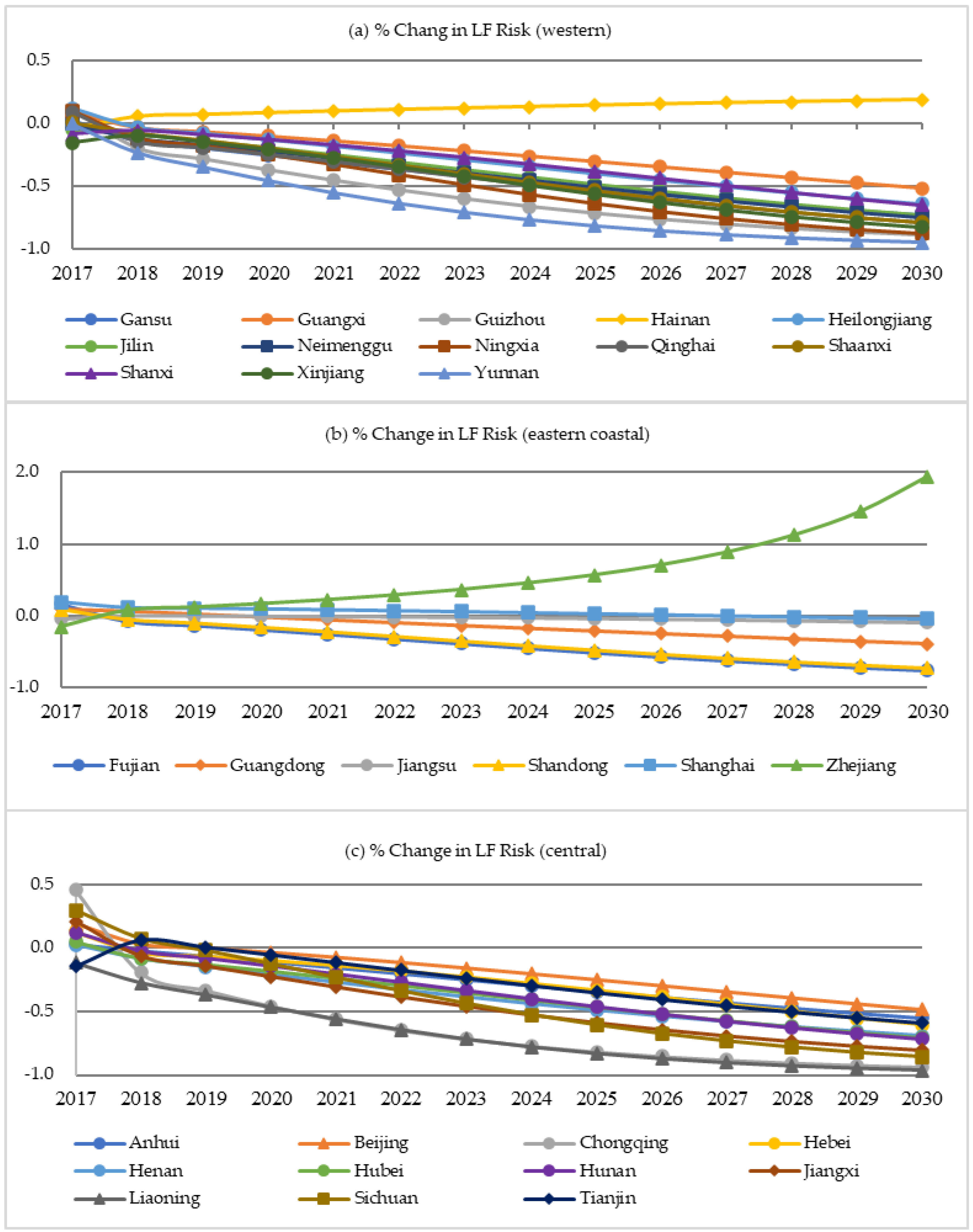
Using a grey forecasting GM(1,1) model, we predict the severity of land finance risks in the next decade. Figure 10 depicts the risk early warnings for the year 2030. It predicts that most provinces will be at low risk levels in 2030, whereas a few provinces such as Beijing, Guangdong, Guangxi, Hunan, Sichuan, Henan, and Anhui will still be at a moderate or severe risk level. Individual provinces such as Guangdong and Guangxi in South China will continue facing an increasing land finance risk in 2030 due to the dense population, lower-end industry, and/or the shortage of developable land. We further show the annual changes in land finance risk for the three sub-zone from 2017 to 2030 in Figure 11. The results indicate that the declining rate of land finance risks is quicker in the central areas than in the western and eastern coastal areas. Hainan’s change in risk will be flattened, while the change in risk in Zhejiang province will even accelerate in the next decade. The results imply that during the social and economic transition, most local governments are beginning to reduce their reliance on land finance. A province is able to reduce its land finance risk if it can timely adjust the policies of land use and find alternative revenue.
5. Policy Implications
Land finance risk management is a complex issue since risk factors may correlate with each other. Recognizing the shortcomings of land finance and its key risk factors, our study provides valuable references to policymakers and government officials. In this section, we discuss the policy implications of our findings and provide suggestions on land finance risk management based on the Chinese background.
From the perspective of social and economic risks, local governments should actively seek more effective land management models. First, the role of local government in social and economic development should be transferred from “city operators” to “public managers”. Local finance revenue should mainly be obtained through taxes and used in the areas of education, social security, public health, and safety, etc. Second, the tax structure of local governments should be adjusted to enhance the stability of local finance revenue and improve the quality of economic growth. The proportion of direct land tax revenue in government revenue should be reduced to avoid local governments’ excessive dependence on land finance. Third, the structure of the land market and the fairness of land trading should be more strictly supervised.
From the perspective of legal risk, more attention should be paid to the delinquencies related to land use and management. First, the administrative performance evaluation standards for local officials should be connected not only to the GDP growth and profits, but also to the quality of economy growth and people’s welfare. Second, more attention should be paid to the improvement of the land use laws and regulations.
From the perspective of ecological risk, it is essential to reduce ecological destruction and its corresponding negative effects. Regional differences should be considered when supplying land resources. Additionally, more attention should be paid to the scientific spatial planning based on quantity indicators of construction land, especially in eastern coastal areas, where construction land resources are inadequate due to rapid urban expansion.
Our spatial spillover effects analysis reveals that there exists inter-provincial imitation and collaboration but no competition. Land users do not switch to the nearby province because of a price advantage as expected. In other words, the land finance market in China is a tightly government-supervised market. A market that lacks free competition may lead to overpricing, but it can also improve stability if the market is manipulated properly.
6. Conclusions
In this study, we developed a framework to explore the spatial-temporal evolution of land finance and assess key land finance risk factors. We defined a measure of land finance that considers both tax and non-tax revenue and revenue from mortgage and financing of land. Based on the provincial-level panel data in the last two decades, we investigated the spatial and temporal variation of land finance across thirty provinces in China. We proposed a four-dimensional risk matrix and assessed land finance risks through spatial panel regression. In addition, using a grey forecasting GM(1,1) model, we predicted the severity of land finance risks in the next decade. We provided suggestions on land finance risk management based on our findings.
In the temporal analysis, we divided the whole period into three stages for land finance: slow growth stage (2001–2008), rapid growth stage (2009–2012), and the fluctuation decline stage (2013–2016). During the period of study, the variation of land finance showed a declining trend with fluctuation. In the spatial analysis, we observed that the spatial variation of land finance decreased from east to west. The results of the spatial analysis showed that land finance had significant positive spatial autocorrelation and obvious spatial clustering characteristics. In addition, the spatial distribution of land finance was consistent with the population-based Hu Line.
Our risk assessment based on four-dimensional risk matrix (i.e., economic risk, social risk, legal risk, and ecological risk) found that the key risk factors presented significant spatial and temporal differences. Our results through spatial panel regressions showed that land finance risks increased and then decreased in most provinces during the study period. Land finance risks fluctuated greatly in the developed coastal provinces, whereas these risks were mainly declining in the underdeveloped western provinces. Furthermore, we examined if there exist spatial spillover effects. Our direct and indirect effects results indicate that there exist spillover effects among adjacent provinces due to the imitation and collaboration. The subzone models revealed more information than the national model by recognizing the spatial differences among the three subzones. The results from substage models also show temporal differences between the two substages, indicating that there were significant structural changes during these two substages.
Using GM(1,1) model, our land finance risk forecast indicates that in the next decade, most provinces will be at a low risk level except some southwest provinces including Guangdong, Beijing, Sichuan, Hainan, and Anhui. In the future, mitigating land finance risks should focus more on developing innovative land management modes, improving performance evaluation standards for local government officials, strengthening dynamic monitoring of cultivated land, and adjusting the supply structure of construction land.
The future study can be extended in many ways. First, classifying land finance risk factors into economic risk, social risk, legal risk, and ecological risk is subjective and worth revisiting. Second, although the GM(1,1) model has advantages for small samples and short time series datasets, it fails to consider the interaction between land finance and its risk factors. Therefore, more risk assessment models (e.g., neural networks and Markov chain models) can be examined in the future to check if they could better fit land finance analysis.
Supplementary Materials
The following supporting information can be downloaded at: https://www.mdpi.com/article/10.3390/risks10100196/s1, Supplementary Materials I: Table S1: Pairwise comparison matrix of the land finance factors; Table S2: Three subzones of land finance by the k-means clustering method; Table S3: Land finance risks during 2009–2016; Table S4: Four types of land finance risks during 2009–2016; Table S5 Fixed-effect and random-effect models with year dummy variables; Table S6 Comparison of the results using normalize vs. unnormalized data. Supplementary Materials II: Figure S1 Scatter Plots between land finance and significant risk factors in years 2009–2016.
Author Contributions
D.Z.—Conceptualization, methodology, software, data collection, data management, investigation, original draft, and paper revision; R.T.—Conceptualization, methodology, investigation, data analysis, writing—original draft preparation, and paper revision; Z.L.—Writing—original draft preparation and paper revision; L.L.—Conceptualization and methodology; J.W.—Software and data analysis, S.F.—Data collection and data curation. All authors have read and agreed to the published version of the manuscript.
Funding
This work is supported by the National Social Science Fund of China (19BGL283).
Data Availability Statement
The data presented in this study are available upon request from the corresponding author.
Conflicts of Interest
The authors declare no conflict of interest.
| 1 | Generally, to scale variable into interval , we apply the formula where is the normalized value of (Basheera and Hajmeerb 2000). We normalize the original data into the interval to ensure the calculation of in the entropy method (Equation (15)) meaningful. |
| 2 | The province Xizang was excluded due to data availability. |
| 3 | http://www.ngcc.cn (accessd on 10 December 2021) |
| 4 | In March 2018, the Ministry of Natural Resources was established in accordance with the Institutional Reform Plan of the State Council approved at the first meeting of the 13th National People’s Congress; the responsibilities of the Ministry of Land and Resources were compiled into the newly established Ministry. The Ministry of Land and Resources was then no longer be retained. |
| 5 | The Notice on Regulating the State-Owned Land Use Rights Transfer Payments Management (The General Office of the State Council of the People’s Republic of China 2007). |
| 6 | The Notice on Improving the Level of Cultivated Land Protection and Comprehensively Strengthening the Construction and Management of Cultivated Land Quality (The Land Improvement Center of Ministry of Land and Resources 2012). |
| 7 | Hu Line was first identified by Dr. Huanyong Hu in 1935 (Hu 1935). |
| 8 | For more details in the three zones, see Table S3 in Supplementary Materials I. |
| 9 | Based on the LM test results reported in Table 4, we include only the spatial-fixed effects, but not the time-fixed effects in the fixed-effect regression. |
| 10 | We also investigate the models that include year dummy variables. The corresponding results from specifications [1]–[3] in Table 5 with year dummies are reported in Table S5 in Supplementary Materials I. Adding these year dummies does not affect the conclusion in risk assessment of land finance, except it slightly increases the of the fixed-effect model and significantly increases the of the random-effect model. |
| 11 | Due to the data availability, we conduct substage regressions based only on data of 2009–2016 (Stages 2 and 3). |
References
- Anselin, Luc. 1995. Local indicators of spatial association—LISA. Geographical Analysis 27: 93–115. [Google Scholar] [CrossRef]
- Anselin, Luc, Julie Le Gallo, and Hubert Jayet. 2008. Spatial panel econometrics. Spatial Panel Econometrics. In Advanced Studies in Theoretical and Applied Econometrics. Edited by László Mátyás and Patrick Sevestre. Berlin: Springe, pp. 625–60. [Google Scholar]
- Basheera, I. A., and M. Hajmeerb. 2000. Artificial neural networks: Fundamentals, computing, design, and application. Journal of Microbiological Methods 43: 3–31. [Google Scholar] [CrossRef]
- Cai, Meina, Pengfei Liu, and Hui Wang. 2020. Political trust, risk preferences, and policy support: A study of land dispossessed villagers in China. World Development 125: 104687. [Google Scholar] [CrossRef]
- Chen, Wendy Y., and Fox Zhi Yong Hu. 2015. Producing nature for public: Land-based urbanization and provision of public green spaces in China. Applied Geography 58: 32–40. [Google Scholar] [CrossRef]
- Chen, Zhigang, Jing Tang, Jiayu Wan, and Yi Chen. 2017. Promotion incentives for local officials and the expansion of urban construction land in china: Using the Yangtze river delta as a case study. Land Use Policy 63: 214–25. [Google Scholar] [CrossRef]
- Deng, Ju-Long. 1982. Control problems of grey systems. Systems & Control Letters 1: 288–94. [Google Scholar] [CrossRef]
- Du, Jinfeng, and Richard B. Peiser. 2014. Land supply, pricing and local governments’ land hoarding in China. Regional Science and Urban Economics 48: 180–89. [Google Scholar] [CrossRef]
- Elhorst, J. Paul. 2010. Spatial Panel Data Models. In Handbook of Applied Spatial Analysis. Edited by Manfred M. Fischer and Arthur Getis. Berlin: Springer, pp. 377–407. [Google Scholar] [CrossRef]
- Foglia, Matteo, and Eliana Angelini. 2019. The Time-Spatial Dimension of Eurozone Banking Systemic Risk. Risks 7: 75. [Google Scholar] [CrossRef] [Green Version]
- Fu, Qiang. 2015. When fiscal recentralization meets urban reforms: Prefectural land finance and its association with access to housing in urban China. Urban Studies 52: 1791–809. [Google Scholar] [CrossRef]
- Fu, Qiang, and Nan Lin. 2013. Local state marketism: An institutional analysis of China’s urban housing and land market. Chinese Sociological Review 46: 3–24. [Google Scholar] [CrossRef]
- Gao, Jinlong, Yehua Dennis Wei, Wen Chen, and Jianglong Chen. 2014. Economic transition and urban land expansion in Provincial China. Habitat International 44: 461–73. [Google Scholar] [CrossRef]
- Geng, Bin, Xiaoling Zhang, Ying Liang, Haijun Bao, and Martin Skitmore. 2018. Sustainable land finance in a new urbanization context: Theoretical connotations, empirical tests and policy recommendations. Resources, Conservation and Recycling 128: 336–44. [Google Scholar] [CrossRef] [Green Version]
- Getis, Arthur, and J. Keith Ord. 1992. The analysis of spatial association by use of distance statistics. Geographical Analysis 24: 189–206. [Google Scholar] [CrossRef]
- Gong, Zaiwu, and Jeffrey Yi-Lin Forrest. 2014. Special issue on meteorological disaster risk analysis and assessment: On basis of grey systems theory. Natural Hazards 71: 995–1000. [Google Scholar] [CrossRef] [Green Version]
- Guo, Gang. 2009. China’s local political budget cycles. American Journal of Political Science 53: 621–32. [Google Scholar] [CrossRef]
- Han, Li, and James Kai-Sing Kung. 2015. Fiscal incentives and policy choices of local governments: Evidence from China. Journal of Development Economics 116: 89–104. [Google Scholar] [CrossRef]
- Han, Wenjing, Xiaoling Zhang, and Zhengfeng Zhang. 2019. The role of land tenure security in promoting rural women’s empowerment: Empirical evidence from rural China. Land Use Policy 86: 280–89. [Google Scholar] [CrossRef]
- He, Canfei, Yi Zhou, and Zhiji Huang. 2016. Fiscal decentralization, political centralization, and land urbanization in China. Urban Geography 37: 436–57. [Google Scholar] [CrossRef]
- He, Chunyang, Norio Okada, Qiaofeng Zhang, Peijun Shi, and Jingshui Zhang. 2006. Modeling urban expansion scenarios by coupling cellular automata model and system dynamic model in Beijing, China. Applied Geography 26: 323–45. [Google Scholar] [CrossRef]
- Hu, Huanyong. 1935. Distribution of China’s population: Accompanying charts and density map. Acta Geographica Sinica 2: 33–74. (In Chinese). [Google Scholar]
- Hu, Fox Z. Y., and Jiwei Qian. 2017. Land-based finance, fiscal autonomy, and land supply for affordable housing in urban China: A prefecture-level analysis. Land Use Policy 69: 454–60. [Google Scholar] [CrossRef]
- Huang, Dingxi, and Roger C. K. Chan. 2018. On ‘Land Finance’ in urban China: Theory and practice. Habitat International 75: 96–104. [Google Scholar] [CrossRef]
- Huang, Zhiji, Yehua Dennis Wei, Canfei He, and Han Li. 2015. Urban land expansion under economic transition in China: A multilevel modeling analysis. Habitat International 47: 69–82. [Google Scholar] [CrossRef]
- Hui, Eddie Chi Man, Hai Jun Bao, and Xiao Ling Zhang. 2013. The policy and praxis of compensation for land expropriations in China: An appraisal from the perspective of social exclusion. Land Use Policy 32: 309–16. [Google Scholar] [CrossRef]
- Javed, Saad Ahmed, and Sifeng Liu. 2018. Predicting the research output/growth of selected countries: Application of Even GM (1,1) and NDGM models. Scientometrics 115: 395–413. [Google Scholar] [CrossRef]
- Jia, Junxue, Qingwang Guo, and Jing Zhang. 2014. Fiscal decentralization and local expenditure policy in China. China Economic Review 28: 107–22. [Google Scholar] [CrossRef]
- Jin, Cheng, and Yuqi Lu. 2009. Evolvement of spatial pattern of economy in Jiangsu province at county level. Acta Geographica Sinica 64: 713–24. [Google Scholar]
- Li, Pei, Yi Lu, and Jin Wang. 2016. Does flattening government improve economic performance? Evidence from China. Journal of Development Economics 123: 18–37. [Google Scholar] [CrossRef]
- Li, Tingting, Hualou Long, Shuangshuang Tu, and Yanfei Wang. 2015. Analysis of income inequality based on income mobility for poverty alleviation in rural China. Sustainability 7: 16362–78. [Google Scholar] [CrossRef] [Green Version]
- Li, Yan, and Chao Peng. 2018. Research on the causes and responsive measures of China’s fiscal expenditure solidification. Journal of World Economic Research 7: 82–91. [Google Scholar] [CrossRef]
- Lian, Hongping, and Raul P. Lejano. 2014. Interpreting Institutional Fit: Urbanization, Development, and China’s “Land-Lost”. World Development 61: 1–10. [Google Scholar] [CrossRef]
- Liu, Tao, and George C. S. Lin. 2014. New geography of land commodification in Chinese cities: Uneven landscape of urban land development under market reforms and globalization. Applied Geography 51: 118–30. [Google Scholar] [CrossRef]
- Liu, Yansui, Lijuan Wang, and Hualou Long. 2008. Spatio-temporal analysis of land-use conversion in the eastern coastal China during 1996–2005. Journal of Geographical Sciences 18: 274–82. [Google Scholar] [CrossRef]
- Lu, Juan, Bin Li, and He Li. 2019. The influence of land finance and public service supply on peri-urbanization: Evidence from the counties in China. Habitat International 92: 102039. [Google Scholar] [CrossRef]
- Ma, Shuang, and Ren Mu. 2020. Forced off the farm? Farmers’ labor allocation response to land requisition in China. World Development 132: 104980. [Google Scholar] [CrossRef]
- Meng, Hao, Xianjin Huang, Hong Yang, Zhigang Chen, Jun Yang, Yan Zhou, and Jianbao Li. 2019. The influence of local officials’ promotion incentives on carbon emission in Yangtze River Delta, China. Journal of Cleaner Production 213: 1337–45. [Google Scholar] [CrossRef]
- Mullan, Katrina, Pauline Grosjean, and Andreas Kontoleon. 2011. Land Tenure Arrangements and Rural–Urban Migration in China. World Development 39: 123–33. [Google Scholar] [CrossRef]
- Pan, Fenghua, Fengmei Zhang, Shengjun Zhu, and Dariusz Wójcik. 2017. Developing by borrowing? Interjurisdictional competition, land finance and local debt accumulation in China. Urban Studies 54: 897–916. [Google Scholar] [CrossRef]
- Pan, Jiun-Nan, Jr-Tsung Huang, and Tsun-Feng Chiang. 2015. Empirical study of the local government deficit, land finance and real estate markets in China. China Economic Review 32: 57–67. [Google Scholar] [CrossRef]
- Qi, Wei, Shenghe Liu, Meifeng Zhao, and Zhen Liu. 2016. China’s different spatial patterns of population growth based on the “Hu Line”. Journal of Geographical Sciences 26: 1611–25. [Google Scholar] [CrossRef]
- Qin, Yu, Hongjia Zhu, and Rong Zhu. 2016. Changes in the distribution of land prices in urban China during 2007–12. Regional Science and Urban Economics 57: 77–90. [Google Scholar] [CrossRef]
- Saaty, Thomas L. 1994. How to make a decision: The analytic hierarchy process. European Journal of Operational Research 24: 19–43. [Google Scholar] [CrossRef]
- Shannon, Claude E., and Warren Weaver. 1949. The mathematical theory of communication. Chicago: University of Illinois Press. [Google Scholar]
- Shi, Yaobo, Chun-Ping Chang, Chyi-Lu Jang, and Yu Hao. 2018. Does economic performance affect officials’ turnover? Evidence from municipal government leaders in China. Quality & Quantity 52: 1873–91. [Google Scholar] [CrossRef]
- Smith, Graeme. 2013. Measurement, promotions and patterns of behavior in Chinese local government. Journal of Peasant Studies 40: 1027–50. [Google Scholar] [CrossRef]
- Su, Shiliang, Dan Li, Xiang Yu, Zhonghao Zhang, Qi Zhang, Rui Xiao, Junjun Zhi, and Jiaping Wu. 2011. Assessing land ecological security in Shanghai (China) based on catastrophe theory. Stochastic Environmental Research & Risk Assessment 25: 737–46. [Google Scholar] [CrossRef]
- Tang, Peng, Xiaoping Shi, Jinlong Gao, Shuyi Feng, and Futian Qu. 2019. Demystifying the key for intoxicating land finance in China: An empirical study through the lens of government expenditure. Land Use Policy 85: 302–9. [Google Scholar] [CrossRef]
- Tao, Ran, Fubing Su, Mingxing Liu, and Guangzhong Cao. 2010. Land leasing and local public finance in China’s regional development: Evidence from prefecture-level cities. Urban Studies 47: 2217–36. [Google Scholar] [CrossRef]
- The General Office of the State Council of the People’s Republic of China. 2007. The Notice on Regulating the State-Owned Land Use Rights Transfer Payments Management. Available online: http://www.gov.cn/zwgk/2006-12/25/content_478251.htm (accessed on 6 June 2020).
- The Land Improvement Center of Ministry of Land and Resources. 2012. Notice on Improving the Level of Cultivated Land Protection and Comprehensively Strengthening the Construction and Management of Cultivated Land Quality. Beijing: The Land Improvement Center of Ministry of Land and Resources. [Google Scholar]
- Tsui, Kai Yuen. 2011. China’s infrastructure investment boom and local debt crisis. Eurasian Geography and Economics 52: 686–711. [Google Scholar] [CrossRef]
- Wang, De, Li Zhang, Zhao Zhang, and Simon Xiaobin Zhao. 2011. Urban infrastructure financing in reform-era China. Urban Studies 48: 2975–98. [Google Scholar] [CrossRef]
- Wang, Hong, Zhiqiu Gao, Jingzheng Ren, Yibo Liu, Lisa Tzu-Chi Chang, Kevin Cheung, Yun Feng, and Yubin Li. 2018. An urban-rural and sex differences in cancer incidence and mortality and the relationship with PM2.5 exposure: An ecological study in the southeastern side of Hu line. Chemosphere 216: 766–73. [Google Scholar] [CrossRef]
- Wang, Shaojian, Chuanglin Fang, and Yang Wang. 2016. Spatiotemporal variations of energy-related CO2 emissions in China and its influencing factors: An empirical analysis based on provincial panel data. Renewable and Sustainable Energy Reviews 55: 505–15. [Google Scholar] [CrossRef]
- Wang, Wen, and Fangzhi Ye. 2016. The political economy of land finance in China. Public Budgeting & Finance 36: 91–110. [Google Scholar] [CrossRef]
- Wang, Yiming, and Steffanie Scott. 2013. Illegal farmland conversion in China’s urban periphery: Local regime and national transitions. Urban Geography 29: 327–47. [Google Scholar] [CrossRef]
- Wen, Haizhen, and Yunlong Tao. 2015. Polycentric urban structure and housing price in the transitional China: Evidence from Hangzhou. Habitat International 46: 138–46. [Google Scholar] [CrossRef]
- Wu, Fulong. 2014. Commodification and housing market cycles in Chinese cities. Journal International Journal of Housing Policy 15: 6–26. [Google Scholar] [CrossRef] [Green Version]
- Wu, Qun, Yongle Li, and Siqi Yan. 2015. The incentives of China’s urban land finance. Land Use Policy 42: 432–42. [Google Scholar] [CrossRef]
- Xu, Nannan. 2019. What gave rise to China’s land finance? Land Use Policy 87: 104015. [Google Scholar] [CrossRef]
- Yang, X. Jin. 2013. China’s Rapid Urbanization. Science 342: 310. [Google Scholar] [CrossRef]
- Ye, Fangzhi, and Wen Wang. 2013. Determinants of land finance in China: A study based on provincial-level panel data. Australian Journal of Public Administration 72: 293–303. [Google Scholar]
- Yuan, Chaoqing, Sifeng Liu, and Zhigeng Fang. 2016. Comparison of China’s primary energy consumption forecasting by using ARIMA (the autoregressive integrated moving average) model and GM(1,1) model. Energy 100: 384–90. [Google Scholar] [CrossRef]
- Zhang, Bangbang, Jiaxiang Li, Wenmiao Tian, Haibin Chen, Xiangbin Kong, Wei Chen, Minjuan Zhao, and Xianli Xia. 2020. Spatio-temporal variances and risk evaluation of land finance in China at the provincial level from 1998 to 2017. Land Use Policy 99: 104804. [Google Scholar] [CrossRef]
- Zhang, Ting-Ting, Sheng-Lan Zeng, Yu Gao, Zu-Tao Ouyang, Bo Li, Chang-Ming Fang, and Bin Zhao. 2011. Assessing impact of land uses on land salinization in the Yellow River Delta, China using an integrated and spatial statistical model. Land Use Policy 28: 857–66. [Google Scholar] [CrossRef]
- Zhang, Tingwei. 2000. Land market forces and government’s role in sprawl—The case of China. Cities 17: 123–35. [Google Scholar] [CrossRef]
- Zheng, Heran, Xin Wang, and Shixiong Cao. 2014. The land finance model jeopardizes China’s sustainable development. Habitat International 44: 130–36. [Google Scholar] [CrossRef]
- Zhong, Taiyang, Xiaoling Zhang, Xianjin Huang, and Fang Liu. 2019. Blessing or curse? Impact of land finance on rural public infrastructure development. Land Use Policy 85: 130–41. [Google Scholar] [CrossRef]
- Zhou, De, Jianchun Xu, Li Wang, and Zhulu Lin. 2015. Assessing urbanization quality using structure and function analyses: A case study of the urban agglomeration around Hangzhou Bay (UAHB), China. Habitat International 49: 165–76. [Google Scholar] [CrossRef]
- Zhou, De, Zhulu Lin, and Siew Hoon Lim. 2019. Spatial characteristics and risk factor identification for land use spatial conflicts in a rapid urbanization region in China. Environmental Monitoring and Assessment 191: 677. [Google Scholar] [CrossRef] [PubMed]
- Zhou, De, Zhulu Lin, Liming Liu, and David Zimmermann. 2013. Assessing secondary soil salinization risk based on the PSR sustainability framework. Journal of Environmental Management 128: 642–54. [Google Scholar] [CrossRef]
- Zhou, Wei, and Jian-Min He. 2013. Generalized GM (1,1) model and its application in forecasting of fuel production. Applied Mathematical Modelling 37: 6234–43. [Google Scholar] [CrossRef]
Figure 1.
The proportions of financial revenue (a) and expenditure (b) between central and local governments.
Figure 1.
The proportions of financial revenue (a) and expenditure (b) between central and local governments.
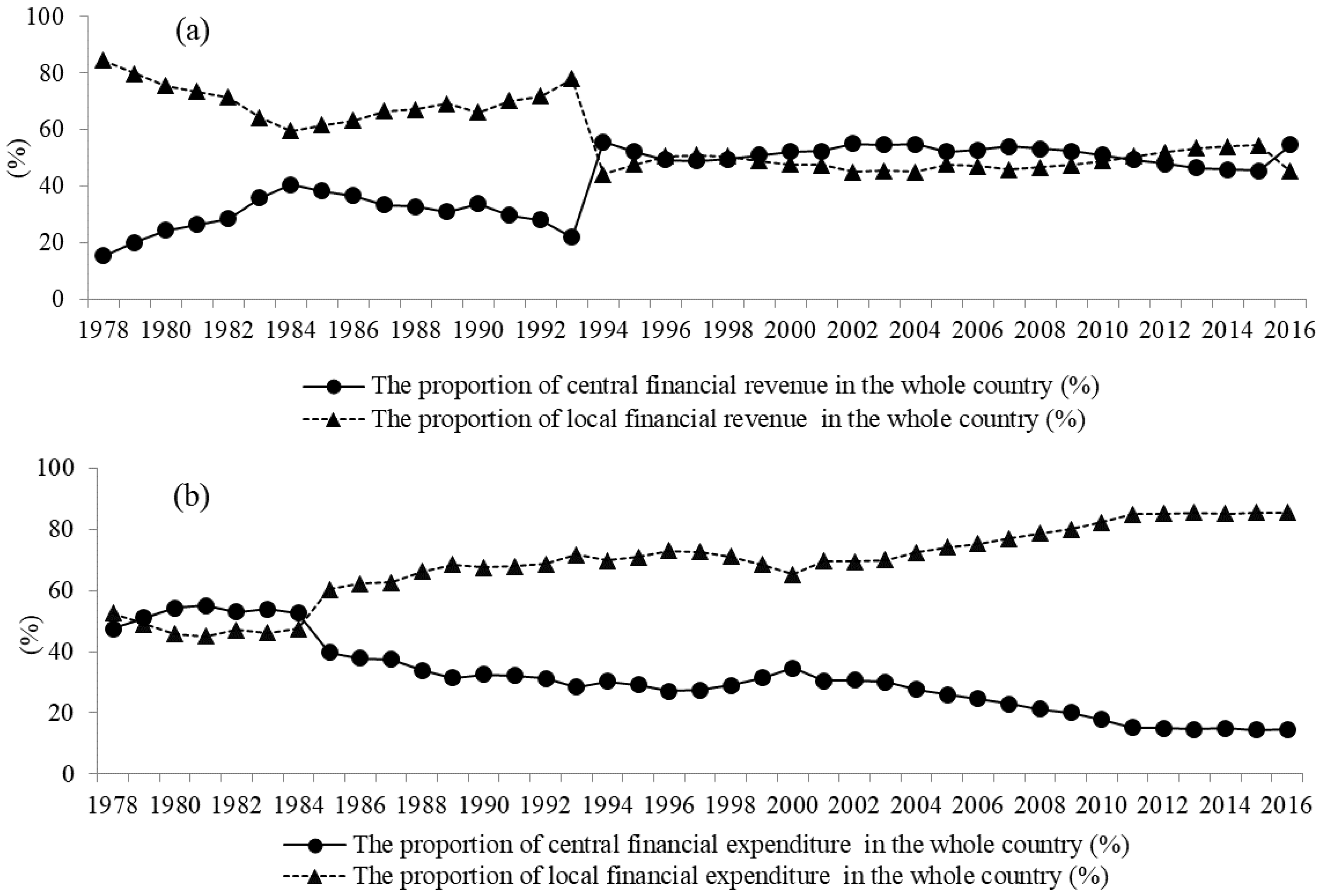
Figure 2.
The composition of the measurement of land finance.

Figure 3.
The four-dimensional risk matrix of land finance.
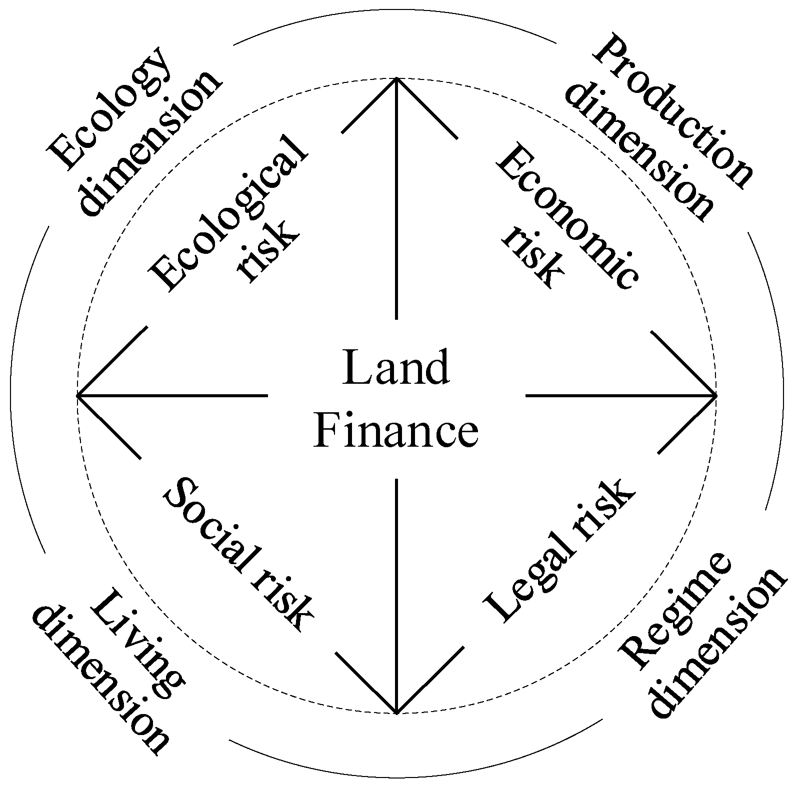
Figure 4.
The trend of annual land finance in Stage 1 (2001–2008), Stage 2 (2009–2012), and Stage 3 (2013–2016), respectively.
Figure 4.
The trend of annual land finance in Stage 1 (2001–2008), Stage 2 (2009–2012), and Stage 3 (2013–2016), respectively.
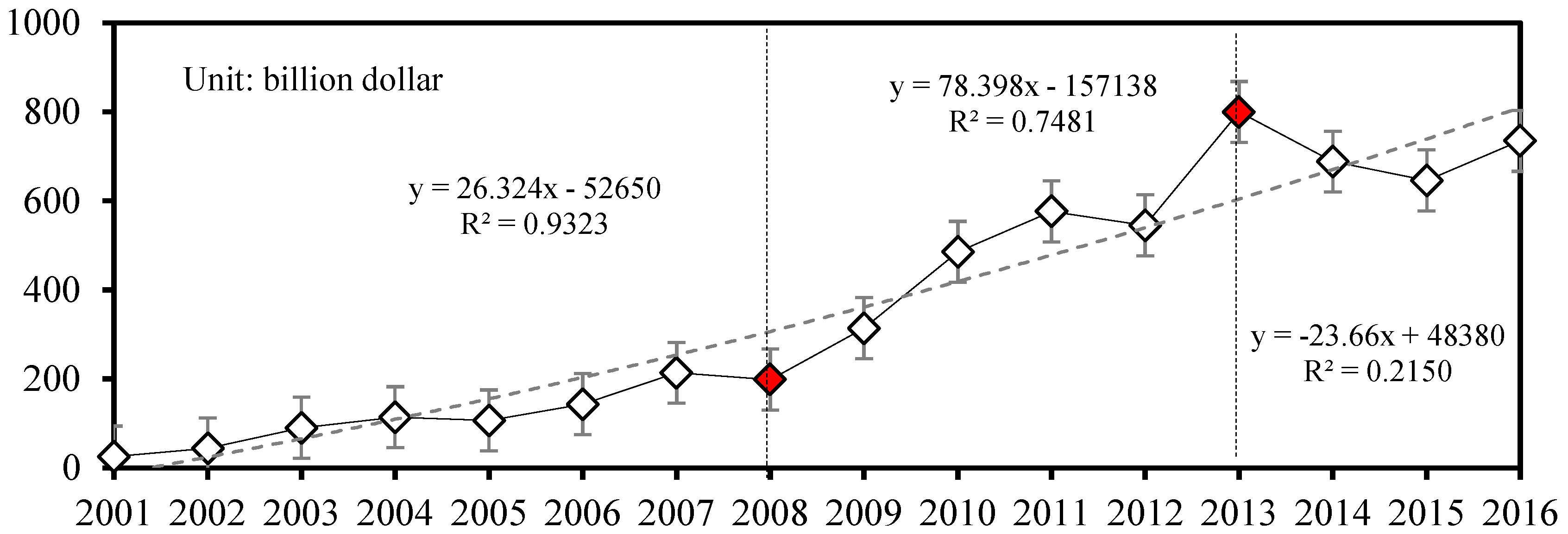
Figure 5.
Spatial pattern of average growth index of land finance of the thirty provinces in stages one, two, and three.
Figure 5.
Spatial pattern of average growth index of land finance of the thirty provinces in stages one, two, and three.
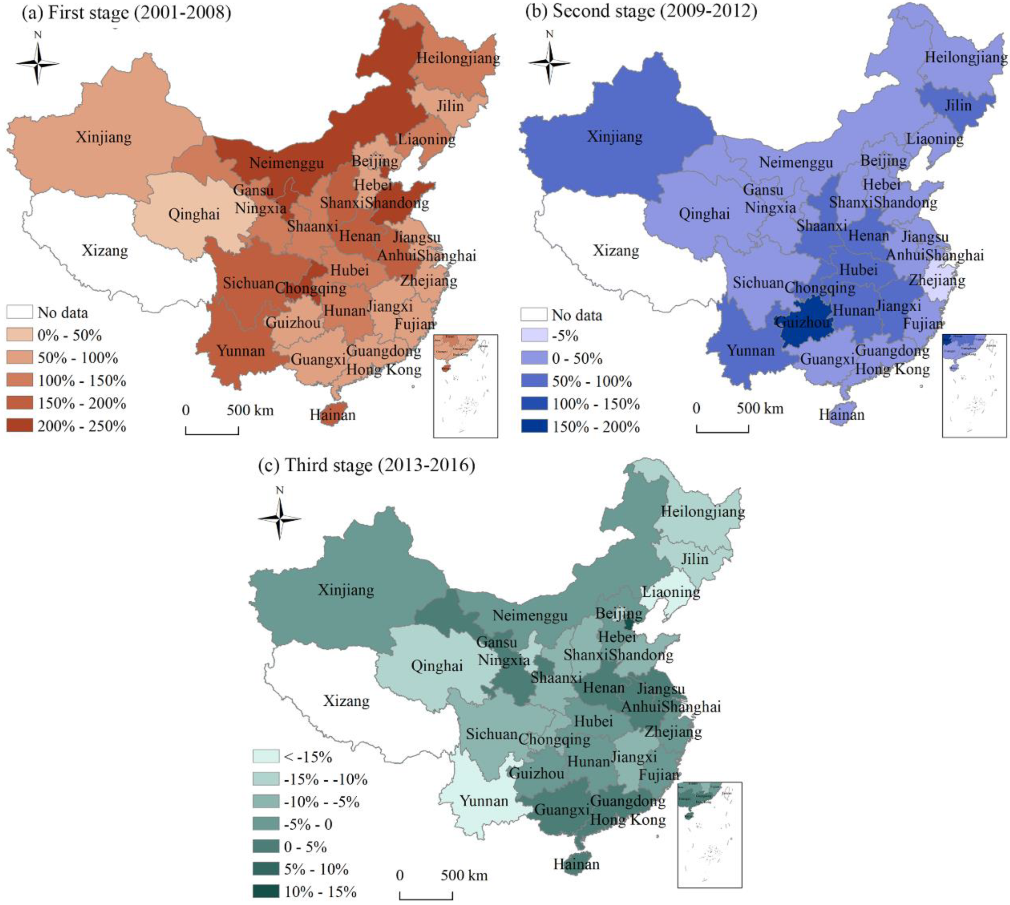
Figure 6.
Average growth index of land finance of the thirty provinces in stage one, two, and three (primary axis (left) for the first stage and second stage, secondary axis (right) for the third stage).
Figure 6.
Average growth index of land finance of the thirty provinces in stage one, two, and three (primary axis (left) for the first stage and second stage, secondary axis (right) for the third stage).

Figure 7.
The spatial and temporal evolution of China’s land finance (Zone 1—Western areas, Zone 2—Central areas, and Zone 3—Eastern coastal areas).
Figure 7.
The spatial and temporal evolution of China’s land finance (Zone 1—Western areas, Zone 2—Central areas, and Zone 3—Eastern coastal areas).
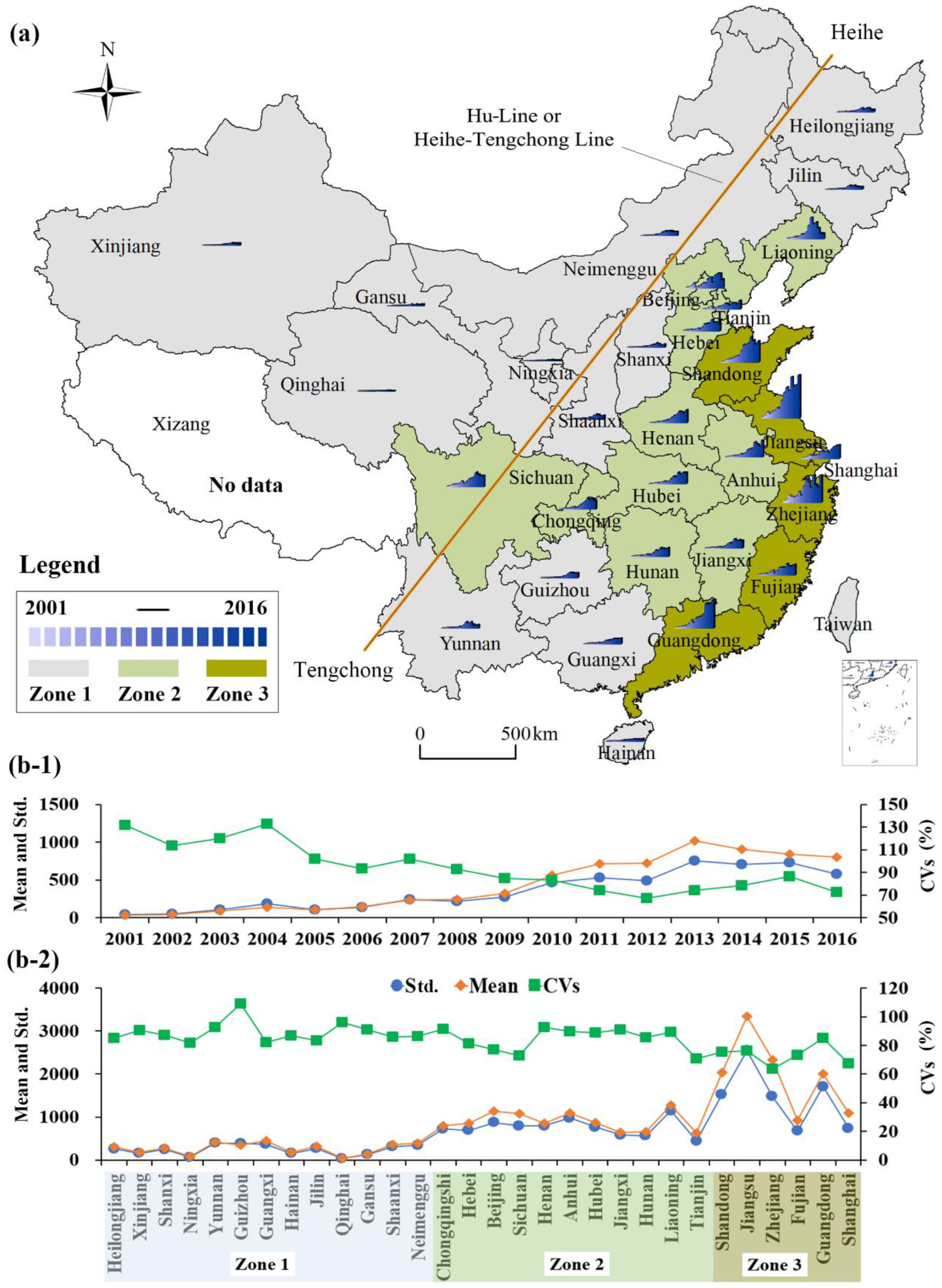
Figure 8.
The spatial pattern and temporal evolution of land finance risks from 2009 to 2016.

Figure 9.
The spatial and temporal evolution of four types of risks.

Figure 10.
Early warning and dynamic changes of land finance risk.

Figure 11.
Annual change in land finance risks from 2017 to 2030.

Table 1.
Selected indicators for land finance risks assessment based on the four-dimensional risk matrix.
Table 1.
Selected indicators for land finance risks assessment based on the four-dimensional risk matrix.
| Type (C) | Risk Variable (X—Normalized Variable) | Variable Description | Expected Sign | |
|---|---|---|---|---|
| Social risks | X1 | Urbanization rate (%) | The proportion of the population living in urban areas. It represents the urbanization level of a country or region. | + |
| X2 | Increase of developed land (hm2) | The amount of agricultural land and unused land converts to developed land per year. | + | |
| X3 | Average housing price growth rate (%) | The growth rate in year t equals the average price of commodity house in year t minus the average price of commodity house in year t − 1 divided by the average price of commodity house in year t − 1. | + | |
| X4 | The income disparity between urban and rural residents (%) | The ratio of the disposable income of urban residents per capita to the net income of rural residents per capita. The ratio represents the risk of income differentiation between urban and rural residents. | + | |
| X5 | Degree of development of land markets (%) | The proportion of the total amount of land transferred through bidding, auction, and sale, representing the degree of development of land markets. | − | |
| X6 | Cultivated land per capita (hm2/capita) | Cultivated land area/total population, representing cultivated area per capita. | − | |
| Economic risks | X7 | Degree of land transfer dependence (%) | The proportion of land finance scaled by local revenue. It represents the dependence of the local government on land finance. | + |
| X8 | Deficit ratio (%) | The proportion of fiscal deficit in GDP, representing the comparison of the annual revenue and expenditure of local governments. | + | |
| X9 | Macro tax burden (%) | The proportion of government revenue in GDP, representing a country’s overall level of the tax burden and overall economic strength. | + | |
| X10 | The asset-liability ratio of real estate enterprises (%) | The ratio of total ending liabilities to total assets, representing the ability of an enterprise to conduct business activities with funds provided by creditors. | + | |
| Legal risks | X11 | Number of land violation cases (#) | It measures the level of corruption of local government in land management. | + |
| X12 | Number of illegal land occupation cases (#) | It measures the management level of local government in the field of land law enforcement and supervision. | + | |
| X13 | Percentage of cultivated land in illegal occupation cases (%) | It measures the extent of damage to cultivated land resources caused by local government’s illegal occupation. | + | |
| Ecological risks | X14 | Percentage of cultivated land area (%) | The proportion of cultivated land in total land area. | − |
| X15 | Cultivated land decrease rate (%) | The ratio of the annual decrease in cultivated land to the total cultivated land, representing the extent of damage of annual cultivated land. | − | |
Notes: “+” means the positive indicator, “−” means the negative indicator.
Table 2.
Judgment standard of prediction accuracy for the GM(1,1) model.
| Accuracy Level | Small Error Probability (p) | Posterior Error Ratio (c) |
|---|---|---|
| Good | p > 0.95 | < 0.35 |
| Qualified | 0.8 < p ≤ 0.95 | < 0.5 |
| Barely qualified | 0.7 < p ≤ 0.8 | < 0.65 |
| Fail | p ≤ 0.7 |
Table 3.
Spatial autocorrelation indexes of land finance from 2001 to 2016.
| Stages | Year | Moran’s I | p-Value | Getis-Ord G | p-Value | ||
|---|---|---|---|---|---|---|---|
| First stage (2001–2008) | 2001 | 0.2324 | 2.3532 | 0.0220 | 0.2052 | 2.1001 | 0.0357 |
| 2002 | 0.3835 | 3.8478 | 0.0050 | 0.2454 | 3.1507 | 0.0016 | |
| 2003 | 0.3786 | 3.9569 | 0.0050 | 0.2516 | 3.0904 | 0.0020 | |
| 2004 | 0.4436 | 3.9794 | 0.0020 | 0.1937 | 2.3292 | 0.0198 | |
| 2005 | 0.4357 | 4.1799 | 0.0010 | 0.2314 | 3.1887 | 0.0014 | |
| 2006 | 0.3790 | 3.5902 | 0.0040 | 0.2176 | 3.0099 | 0.0026 | |
| 2007 | 0.2386 | 2.3183 | 0.0220 | 0.2008 | 2.4984 | 0.0125 | |
| 2008 | 0.3365 | 3.1345 | 0.0030 | 0.1921 | 2.4350 | 0.0149 | |
| Second stage (2009–2012) | 2009 | 0.3669 | 3.5018 | 0.0040 | 0.2169 | 2.7887 | 0.0053 |
| 2010 | 0.3410 | 3.2383 | 0.0040 | 0.2071 | 2.8024 | 0.0051 | |
| 2011 | 0.2696 | 2.6398 | 0.0090 | 0.1876 | 2.3521 | 0.0187 | |
| 2012 | 0.2598 | 2.5950 | 0.0110 | 0.1947 | 2.8730 | 0.0041 | |
| Third stage (2013–2016) | 2013 | 0.2806 | 2.7945 | 0.0060 | 0.2023 | 3.0680 | 0.0022 |
| 2014 | 0.2748 | 2.7005 | 0.0110 | 0.1933 | 2.8582 | 0.0043 | |
| 2015 | 0.2858 | 2.9026 | 0.0060 | 0.1997 | 2.9262 | 0.0034 | |
| 2016 | 0.3686 | 3.7056 | 0.0030 | 0.2251 | 3.5199 | 0.0004 |
Table 4.
Results of model tests.
| Determinants | Statistics | Determinants | Statistics |
|---|---|---|---|
| LM test spatial error | 7.444 *** | LM test spatial lag | 3.203 * |
| Robust test LM spatial error | 4.468 ** | Robust LM test spatial lag | 0.226 |
| Hausman test | Negative |
Notes: ***, **, * imply statistical significance at the 1%, 5% and 10% level, respectively.
Table 5.
The parameter estimates of risk factors of land finance at the national level.
| Basic Level Indicators (X—Normalized Variable) | Fixed-Effects [1] | Random-Effects [2] | Random-Effects [3] | |
|---|---|---|---|---|
| X1 | Urbanization rate | 0.99 *** | 0.4642 *** | 0.4563 *** |
| (0.139) | (3.4856) | (5.3473) | ||
| X2 | Increase of developed land | 0.12 *** | 0.1483 *** | 0.1552 *** |
| (0.029) | (4.4383) | (4.9131) | ||
| X3 | Average housing price growth rate | 0.03 | −0.0111 | |
| (0.026) | (−0.3778) | |||
| X4 | The income disparity between urban & rural residents | 0.16 *** | 0.052 | |
| (0.056) | (0.8732) | |||
| X5 | Degree of land market development | −0.09 *** | −0.0928 *** | −0.0854 ** |
| (0.035) | (−2.6519) | (−2.5372) | ||
| X6 | Per capita cultivated land | 1.32 * | 0.0906 | |
| (0.795) | (0.8169) | |||
| X7 | Degree of land transfer dependence | 0.29 *** | 0.2669 *** | 0.2606 *** |
| (0.028) | (8.854) | (9.2761) | ||
| X8 | Deficit rate | −0.11 | −0.0305 | |
| (0.116) | (−0.3144) | |||
| X9 | Macro tax burden | 0.39 *** | 0.2264 *** | 0.2291 *** |
| (0.073) | (2.8354) | (2.9582) | ||
| X10 | The asset-liability ratio of real estate enterprises | −0.00 | 0.0745 * | |
| (0.042) | (1.6478) | |||
| X11 | Number of land violation cases | 0.02 | 0.0038 | |
| (0.028) | (0.1212) | |||
| X12 | Number of illegal land occupation cases | 0.08 ** | 0.0864 ** | 0.0808 ** |
| (0.034) | (2.2771) | (2.4077) | ||
| X13 | Percentage of cultivated land in illegal occupation cases | −0.04 | −0.0338 | |
| (0.022) | (−1.3608) | |||
| X14 | Percentage of cultivated land area | −2.39 * | 0.1231 | |
| (1.319) | (1.2962) | |||
| X15 | Cultivated land decrease rate | −0.07 * | −0.0419 | |
| (0.036) | (−1.0392) | |||
| Constant | −0.3173 *** | −0.2109 *** | ||
| (−2.7230) | (−5.4626) | |||
| ) | 0.23 *** | 0.3211 *** | 0.3053 *** | |
| (0.056) | −5.6324 | (5.5732) | ||
| 0.151 | 0.461 | 0.441 | ||
Notes: ***, **, and * mean the significance level of 0.001, 0.01, and 0.05, respectively; the values in parentheses are t values.
Table 6.
Results of the direct, indirect, and total effects.
| Variables | Direct Effects | Indirect Effects | Total Effects |
|---|---|---|---|
| X1 | 0.4826 *** | 0.2120 *** | 0.6946 *** |
| (3.4504) | (2.8132) | (3.4517) | |
| X2 | 0.1511 *** | 0.0677 *** | 0.2188 *** |
| (4.4625) | (2.6900) | (3.9534) | |
| X3 | −0.0082 | −0.0036 | −0.0118 |
| (−0.2829) | (−0.2657) | (−0.2796) | |
| X4 | 0.0535 | 0.0248 | 0.0783 |
| (0.9086) | (0.8819) | (0.9093) | |
| X5 | −0.0943 *** | −0.0418 ** | −0.1361 *** |
| (−2.6796) | (−2.2177) | (−2.6230) | |
| X6 | 0.1010 | 0.0443 | 0.1453 |
| (0.8733) | (0.8212) | (0.8661) | |
| X7 | 0.2746 *** | 0.1218 *** | 0.3965 *** |
| (8.4662) | (3.6707) | (7.0936) | |
| X8 | −0.0360 | −0.0157 | −0.0518 |
| (−0.3618) | (−0.3597) | (−0.3638) | |
| X9 | 0.2421 *** | 0.1046 *** | 0.3467 *** |
| (3.0106) | (2.8163) | (3.1360) | |
| X10 | 0.0771 | 0.0344 | 0.1115 |
| (1.6440) | (1.5054) | (1.6328) | |
| X11 | 0.0031 | 0.0008 | 0.0039 |
| (0.0980) | (0.0569) | (0.0856) | |
| X12 | 0.0913 ** | 0.0414 * | 0.1327 ** |
| (2.1911) | (1.7745) | (2.0949) | |
| X13 | −0.0358 | −0.0160 | −0.0518 |
| (−1.4555) | (−1.3470) | (−1.4434) | |
| X14 | 0.1309 | 0.0584 | 0.1892 |
| (1.3166) | (1.2162) | (1.3045) | |
| X15 | −0.0466 | −0.0199 | −0.0665 |
| (−1.1569) | (−1.0998) | (−1.1544) | |
| 0.4613 | 0.4613 | 0.4613 |
Notes: Standard errors in parentheses, ***, **, * imply statistical significance at the 1%, 5% and 10 % level, respectively.
Table 7.
Sub-models of land finance at the temporal scale and the spatial scale.
| Basic Level Indicators (X) | Zone 1 | Zone 2 | Zone 3 | Stage 2 | Stage 3 |
|---|---|---|---|---|---|
| (Western) | (Central) | (Eastern coastal) | (2009–2012) | (2013–2016) | |
| X1 | 0.0743 | 0.7820 *** | 2.4984 *** | 0.1591 | 0.4986 *** |
| (1.5280) | (5.6217) | (5.9812) | (1.3943) | (3.8610) | |
| X2 | −0.0067 | 0.0564 ** | 0.0569 | 0.1250 *** | 0.1128 *** |
| (−0.4440) | (2.0638) | (1.0797) | (3.4127) | (2.5767) | |
| X3 | −0.0114 | 0.0758 *** | 0.0735 | −0.0361 | 0.0604 |
| (−1.2663) | (2.8920) | (0.9658) | (−1.3251) | (1.4918) | |
| X4 | −0.0638 *** | 0.1153 * | −0.2369 | −0.0401 | −0.0616 |
| (−3.3762) | (1.9566) | (−0.7532) | (−0.4882) | (−0.3569) | |
| X5 | 0.0238 ** | 0.0880 *** | −0.5373 *** | −0.0266 | 0.0586 |
| (2.0121) | (2.6426) | (−3.5224) | (−0.6582) | (1.4548) | |
| X6 | 0.0002 | −3.0799 *** | 15.3790 *** | −0.0410 | −0.0686 |
| (0.0038) | (−2.6226) | (4.7366) | (−0.5715) | (−0.5883) | |
| X7 | 0.1516 *** | 0.3360 *** | 0.6436 *** | 0.2193 *** | 0.4353 *** |
| (14.1764) | (13.6490) | (8.2513) | (6.4781) | (9.8544) | |
| X8 | 0.0005 | −0.2254 | 0.1196 | −0.0996 | −0.0217 |
| (0.0162) | (−1.3303) | (0.1605) | (−1.1050) | (−0.2103) | |
| X9 | 0.0861*** | 0.5962 *** | 1.0444 *** | 0.0114 | 0.0941 |
| (3.7270) | (8.8572) | (4.3906) | (0.1177) | (1.1225) | |
| X10 | −0.0112 | −0.1004 ** | 0.2981 | 0.0770 * | 0.1311 ** |
| (−0.9659) | (−2.3699) | (1.2947) | (1.8345) | (1.9899) | |
| X11 | −0.0037 | −0.0163 | −0.0064 | −0.0120 | −0.0164 |
| (−0.2799) | (−0.8015) | (−0.0922) | (−0.1851) | (−0.5081) | |
| X12 | −0.0094 | 0.0056 | −0.0176 | −0.0564 | 0.0408 |
| (−0.4266) | (0.1806) | (−0.2761) | (−0.7179) | (1.3165) | |
| X13 | 0.0065 | −0.0138 | −0.0535 | 0.0137 | −0.0247 |
| (0.8757) | (−0.7090) | (−0.8270) | (0.4421) | (−0.9511) | |
| X14 | −0.0282 | −0.0862 | −1.2151 *** | 0.0261 | 0.0929 |
| (−0.4866) | (−0.1481) | (−3.2706) | (0.3771) | (0.8823) | |
| X15 | −0.0045 | −0.1000 ** | −0.1621 | 0.0178 | −0.2839 |
| (−0.4319) | (−2.0330) | (−1.0324) | (0.5112) | (−0.3991) | |
| Constant | 0.0774 * | 0.3500 | −3.1251 *** | 0.0071 | −0.1440 |
| (1.8369) | (0.8631) | (−5.1530) | (0.0621) | (−0.3150) | |
| Spatial weights (ρ) | 0.1501 ** | 0.1464 ** | −0.0982 | 0.2562 *** | 0.0536 |
| (2.3648) | (2.0125) | (−1.0179) | (2.7880) | (0.6676) | |
| 0.085 | 0.006 | 0.715 | 0.659 | 0.561 |
Notes: ***, **, and * mean the significance level of 0.001, 0.01, and 0.05, respectively; the values in parentheses are t value test. Both the 3-subzone and 2-satge regressions fit the random-effects models, based on the Hausman tests.
Publisher’s Note: MDPI stays neutral with regard to jurisdictional claims in published maps and institutional affiliations. |
© 2022 by the authors. Licensee MDPI, Basel, Switzerland. This article is an open access article distributed under the terms and conditions of the Creative Commons Attribution (CC BY) license (https://creativecommons.org/licenses/by/4.0/).
Share and Cite
MDPI and ACS Style
Zhou, D.; Tian, R.; Lin, Z.; Liu, L.; Wang, J.; Feng, S. Spatial-Temporal Evolution and Risk Assessment of Land Finance: Evidence from China. Risks 2022, 10, 196. https://doi.org/10.3390/risks10100196
AMA Style
Zhou D, Tian R, Lin Z, Liu L, Wang J, Feng S. Spatial-Temporal Evolution and Risk Assessment of Land Finance: Evidence from China. Risks. 2022; 10(10):196. https://doi.org/10.3390/risks10100196
Chicago/Turabian StyleZhou, De, Ruilin Tian, Zhulu Lin, Liming Liu, Junfeng Wang, and Shijia Feng. 2022. "Spatial-Temporal Evolution and Risk Assessment of Land Finance: Evidence from China" Risks 10, no. 10: 196. https://doi.org/10.3390/risks10100196
Note that from the first issue of 2016, this journal uses article numbers instead of page numbers. See further details here.