Abstract
We analyse four stochastic claims reserving methods in terms of their capability to estimate reserve risk and how successful they are at predicting distributions and VaRs of claim developments in particular. Both actual data and hypothetical claim triangles support our results. The appropriateness of the Solvency II risk margin on a one-year horizon and of the IFRS 17 risk adjustment in the long run largely vary by the chosen risk model. Despite the fact that IFRS 17 does not uniquely prescribe the metric for risk adjustment, we expect that VaR will be widely applied by insurance firms. Overall, actual data suggest that VaRs are predominantly underestimated by the models. Nevertheless, the -VaRs under Solvency II are mostly sufficient on a 10-year-horizon to cover liabilities.
JEL Classification:
G22; C53
1. Introduction
The stochastic nature of values in run-off triangles (and quadrangles) has generally not been examined in traditional non-life reserving. Instead, actuaries have tended to focus on ameliorating the point estimates for ultimate claims. This approach has gradually changed since stochastic claims reserving methods became common practice, see England and Verrall (2002); Wüthrich and Merz (2008). The prediction of future claims’ or payments’ random nature is more and more frequently required in the insurance industry; therefore, the spread of stochastic methods in practice is fairly natural. The estimation of standard deviation, value-at-risk (VaR) and tail value-at-risk (TVaR) have started to become regular exercises in the insurance and financial industries.
England et al. (2019) demonstrates methods for analysing reserve risk and provides models for full predictive claim distribution, which can be applied both for SII and IFRS 17. In the present article, we scrutinise the appropriateness of these models and compare them with two other reserving methods. In essence, stochastic reserving methods forecast probability distributions. Therefore, it is reasonable that we apply tools from the theory of probabilistic forecasts in order to measure the quality of the reserving techniques. The theory of probabilistic forecasting has become widespread in recent years, see Gneiting and Katzfuss (2014); Gneiting et al. (2007). Applications of this theory for non-life claims reserving can be found in Arató et al. (2017), for instance.
We will show that the VaR estimations of the tested methods are generally inaccurate. This result is not surprising: the adequate estimation of the -VaR can hardly be expected based on 50–200 connected data points, let alone of the -VaR. Nevertheless, our view is that this inherent inaccuracy does not necessarily mean that the system is less useful, since the -VaR that the standard formula of SII yields has hardly anything to do with the real -VaR. Yet, the system works. The stochastic reserving methods demonstrated in the present paper reflect on the future’s uncertainty; however, we need to acknowledge their limits.
In the past decade, granular models were established that use policy-by-policy claim development information. These models are referred to as micro models Antonio and Plat (2014). Even more recently, non-linear neural network regression models have started to be explored Wüthrich (2018). Due to the availability of actual observations, we focus on models on run-off triangles.
In terms of structure, after the present introduction, Section 2 compares the predictive performance of four models on real data from Meyers and Shi (2011). The time horizon of forward-looking is one year in accordance with Solvency II. Section 3 repeats the same test of model appropriateness, but on artificially simulated data from log-normal and gamma distributions. Section 4 is the juxtaposition of one-year Solvency II and multi-year IFRS 17 value-at-risk quantiles. Despite the fact that IFRS 17 does not stipulate the exact metric for risk adjustment calculation, we may expect that VaR will be widely applied by insurance institutions. Fully completed triangles (quadrangles), i.e., claim run-offs in the long run are looked at in Section 4 and in more detail in Martinek (2019). Section 5 concludes the paper.
2. Actual Data–Based Validation of Techniques
Several insurance institutions have contributed to the publishing of actual loss data from six business lines Meyers and Shi (2011). We will refer to these data as NAIC data (National Association of Insurance Commissioners). The associated claims occurred during accident years between 1988 and 1997 with a development lag of a maximum of 10 years each. Therefore, each triangle is of the size . In the present analysis, 355 observations have been used, combined from business lines of commercial auto and truck liability and medical insurance (84), medical malpractice—claims made (12), other liability—occurrence (99), private passenger auto liability and medical (88), product liability—occurrence (14), and workers’ compensation (58).
Four models are compared in this paper. The first two can be found in England et al. (2019). These are non-parametric and parametric bootstrapped modifications of the original model Mack (1993), resampling with replacement from the scaled bias adjusted Pearson residuals. The third and the fourth ones are credibility-type models that embed information from a range of observed triangles in the completion of every single triangle, see Martinek (2019). One is based on the over-dispersed Poisson model and the other one is a semi-stochastic model. See Appendix A for a more detailed description of the models.
Value-at-risk is a key metric in SII that determines the solvency capital ratio and consequently the risk margin. We have tested the relation of estimated VaR to the actually observed claims data, see Table 1. Each element of the table reflects the following: Applying a given model one-by-one on the available triangles to calculate the and -VaR, in what percentage of the cases does the estimated VaR exceed the actual observation? All metrics correspond to the claims development result , where (1) stands for the claims reserves at the beginning of calendar year y, (2) denotes the payments made during calendar year y and (3) represents the claims reserves at the end of calendar year y. Similarly, in the multiyear case, (1) and (3) are the beginning and the end of the period reserve, and (2) the payments made in this particular time frame. If a reserving model perfectly fits the underlying characteristics of the data, this value should be exactly the VaR-percentile on average in the corresponding column of the table.

Table 1.
The relation between the estimated VaR and how frequently that number exceeds the actual claim value observation.
We have concluded that all of the observed models underestimate the VaR based on the NAIC data. The most extreme one is the parametric version of the Mack bootstrap, where only of the total ultimate claims are below the -VaRs. The credibility semi-stochastic model performs somewhat better, where this value is vs. the -VaR. Overall, running the four models on the actual data implies a systematic underestimation of VaRs, i.e., the underestimation of the capital requirement and the risk margin.
Subsequently, we look at the claim distributions estimated by the models in comparison with the empirical distributions determined by the actual claims. In probabilistic forecasts -coverage expresses the probability that the observation (from the real distribution) falls into the -central prediction interval of the estimated distribution, see Baran et al. (2013). In other words, with F estimation and G real distribution, -coverage is the G-measure of the central prediction interval of F, i.e.,
In the ideal case when the -coverage value is exactly , see the ideal coverage line in Figure 1. Observe that each of the models are below the ideal identity line, which reinforces the finding pointed out in relation to the VaR, i.e., overly narrow prediction intervals. For instance, the -coverage of the prediction made by the non-parametric Mack bootstrap model is , very similarly to the credibility semi-stochastic () and credibility ODP () methods, and only the parametric Mack bootstrap stands out with .
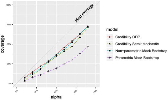
Figure 1.
-coverage with values between and from all business lines combined.
In order to further improve our understanding of the prediction quality, we have visualised the PIT-plots for each model, see Meyers (2015). Firstly, we have calculated the probability integral transform values of each triangle and prediction: , where is the prediction made by the specific model on one triangle and the real observation. Secondly, we have plotted the histogram of . If is governed by for each i, then . Hence, we expect a uniform histogram for a perfect model (as a necessary condition). However, the plots turn out to be non-uniform in Figure 2 and mainly underdispersed ∪-shaped, which implies narrow prediction intervals. In addition, these graphs are asymmetric, meaning that the predictions’ levels of underdispersion are asymmetric.
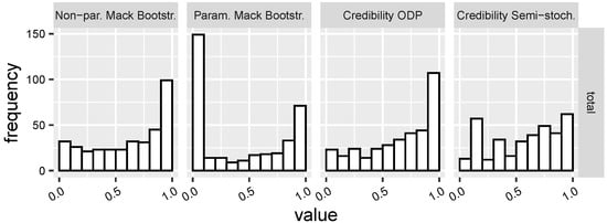
Figure 2.
PIT histograms corresponding to the four reserving models and based on all business lines combined.
Continuous ranked probability scores (CRPS) measure the quality of probabilistic forecasts, see Gneiting and Raftery (2007). By definition, given a prediction F and claim observation x,
We have approximated the expected CRPS by the average of scores resulting from prediction-observation pairs in Table 2. Sporadically, there can be score values with extreme absolute values; therefore, the median scores are also shown in the table. CRPS has its range in and the higher the value, the better the prediction. The best ones, the non-parametric Mack bootstrap and credibility ODP models, perform similarly, trailed by the parametric Mack bootstrap model, and lastly, the credibility semi-stochastic one, which underperforms all of them. (The extreme CRPS is due to an extreme value, see the median for comparison.)
Table 2.
Mean and median CRPS values.
At last, the average width of prediction
expresses the G-expected value of the -central prediction interval’s width determined by F, where F is the predicted distribution and G is the real one, . The lower the average width, the sharper the prediction. Note that this metric is expressed in terms of monetary value. In Figure 3, it can be observed that the Mack bootstrap methods are consistently sharper than the credibility-type methods.
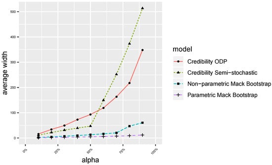
Figure 3.
Average width values for from all business lines.
3. Validation of Techniques from Simulations
Having tested the predictive power of the models on actual data in Section 2, now we simulate fictitious claim histories, i.e., upper triangles and their lower counterparts. Two claim evolution models, the log-normal and the gamma ones, will be used, see Arató et al. (2017). Once these hypothetical observations are done, the validation works in exactly the same manner as in Section 2. The selection of log-normal and gamma models is arbitrary; however, in one form or another these are applied by the insurance industry.
The sample size is 2000, i.e., the number of observed triangles (quadrangles) is significantly larger than in the NAIC database. The number of bootstrapping steps in the Mack bootstrap and credibility ODP models is 200,000 for each triangle. For the initial parameter selection of both log-normal and gamma models, we have estimated the parameters from the triangle published by Taylor and Ashe (1983). This initial run-off triangle has been used exclusively for setting the model parameters.
First, we look at the quality of VaR estimations. When the real claim run-off is governed by the log-normal model, we observe that each of the four estimation methods underestimates the quantiles, see Table 3. In contrast, if the real model is gamma, then both Mack bootstrap models and the credibility ODP model highly overestimate the associated VaRs, see Table 4. Remarkably, the credibility semi-stochastic method consistently underestimates VaRs regardless of the underlying simulation, while it has outperformed all the other estimation methods on real data in Section 2.
Table 3.
Which actual VaR does the estimated VaR approximate if the underlying model is log-normal.
Table 4.
Which actual VaR does the estimated VaR approximate if the underlying model is gamma.
In terms of coverage, Mack bootstrap and credibility ODP models perform reasonably well, see Figure 4 and Figure 5. As we have seen above with VaR estimation performance, the credibility semi-stochastic method is again an outlier compared to the other three, resulting in underdispersed estimations. These findings in the log-normal and gamma simulations, to the contrary, are substantially different than in the case of real observations.
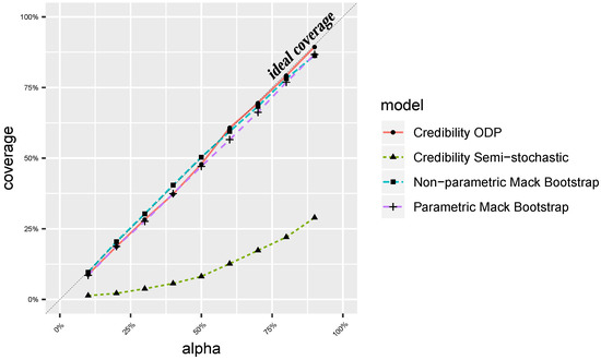
Figure 4.
Coverage values from the log-normal data.
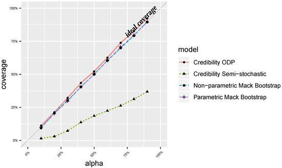
Figure 5.
Coverage values from the gamma data.
For further visualisation of how narrow or good-fit the prediction intervals are, see the PIT histograms in Figure 6 and Figure 7. For the log-normal underlying distribution, all the methods except for the semi-stochastic one (that has ∪-shaped PIT) result in uniform PIT histograms. However, in the case of the gamma distribution, all the methods deviate from the uniform shape. See Appendix B for CRPS and average width figures.
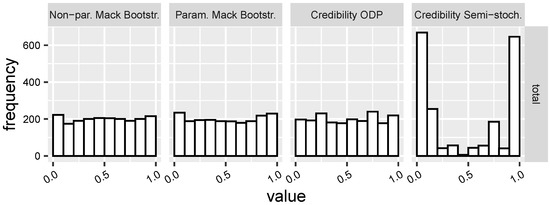
Figure 6.
PIT histograms from the log-normal data.
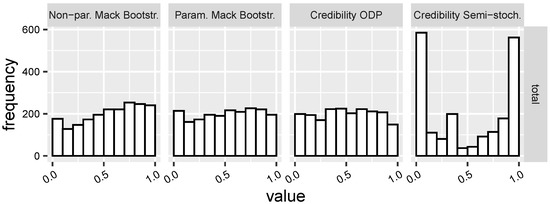
Figure 7.
Histograms of PIT values from the gamma data.
In this section, we have scrutinised claims evolutions with finite higher moments. However, it is interesting to consider the performance of reserving models in the context of distributions with non-finite moments. Denuit and Trufin (2017) presents a case study based on real claims and describes a frequency-severity setting with a discrete mixture severity distribution for each claim size: gamma or inverse Gaussian with probability as a light-tailed component and Pareto type II with probability as a heavy-tailed component.
4. Reconciliation of Solvency II Risk Margin with IFRS 17 Risk Adjustment
In this section, we compare in two ways how the one-year -VaR of SII relates to the multiyear VaR of IFRS 17, i.e., the long-term view of reserve risk. In contrast to SII, the IFRS 17 regime does not stipulate the exact way of risk calculation and how the risk adjustment needs to be determined. Nevertheless, we may assume that a large proportion of market participants will apply either VaR or possibly TVaR for the shocked scenarios.
Firstly, we take a reserving model and , and observe the proportion of actual long-term observations compared to the total where the models’ one-year -VaR would have also been sufficient on the long-run. Secondly, for every method and run-off triangle i, we find which multiyear -VaR is equal to the one-year -VaR. Overall, 50,000 scenarios have been used in the Mack Bootstrap models.
In Table 5, we show how the one-year VaRs relate to the actual observations, i.e., in what ratio they exceed the actually observed payments in the total (10-year) run-off of claims, see Equation (1). In other words, the number of cases where the one-year VaR exceeds the long-run claims development divided by the total number of observations. This table contains comparisons not only for the SII one-year -VaR, but also for the and the ones. For instance, applying the non-parametric Mack Bootstrap method, the resulted -VaR values (in accordance with SII) provided a sufficient capital buffer in of the cases in the long-run. Observe that these values are rather different per estimation method, just as we have seen in Table 1.
Table 5.
The ratio of one-year 99.5%-, 98%- and 95%-VaRs exceeding the multiyear actuals. Results are based on the combined 355 observation from 6 business lines.
In the second comparison, we determine which results in the same multiyear VaR as the -VaR on the NAIC data, i.e., we solve
where the left hand side represents the multiyear and the right hand side the one-year development of claims. The results are based on 355 observations (company per business line) from the NAIC database, and the six business lines contribute to the results combined. In Table 6, these solutions per method are shown. In contrast to the first comparison, the second one produces values. Therefore, each of the four models outlines a distribution of values, and the quartiles, means and medians are incorporated into the table.
Table 6.
Multiyear equivalent of the one-year 99.5%-VaR stemming from the four estimation method (in %).
5. Conclusions
We have tested the accuracy of four stochastic claims reserving models on both actual and hypothetical run-off triangle data. In particular, results show that their capacity to estimate the widely used VaR metrics is generally limited. This finding is in line with our expectations as the size of observation (upper triangle) that provides the basis for the calibration of the future’s estimation is small. Nevertheless, it is reassuring that the -VaR under SII that these models determine is sufficient on a 10-year-horizon for the majority of actually observed cases: for the Non-parametric Mack Bootstrap, for the Parametric Mack Bootstrap, and 92.1%–93.5% for the Credibility ODP and semi-stochastic models. We also emphasise at the same time that these results are higher in every case except for the semi-stochastic one if we determine the VaRs from the simulations themselves rather than from the comparison to known future outcomes.
The appropriate estimation of extreme quantiles such as the -VaR can hardly be expected from any new model. Similar findings have been made in relation to the banking industry, where it is often assumed that the observations are i.i.d. variables, yet the -VaR estimations are highly uncertain from low sample sizes, see Danielsson and Zhou (2016).
Comparing triangle-based models with micro models and machine learning models requires further analysis. We see the testing of such models as the next step in the pursuit of better VaRs.
Author Contributions
Conceptualization, N.M.A. and L.M.; data curation, N.M.A. and L.M.; funding acquisition, N.M.A.; methodology, N.M.A. and L.M.; software, N.M.A. and L.M.; writing—original draft, N.M.A. and L.M.; writing—review and editing, N.M.A. and L.M. All authors have read and agreed to the published version of the manuscript.
Funding
This research has been implemented with the support provided by the Ministry of Innovation and Technology of Hungary from the National Research, Development and Innovation Fund, financed under the ELTE TKP 2021-NKTA-62 funding scheme (project K10602/21).
Data Availability Statement
Data used in Section 2 can be directly downloaded from https://www.casact.org/publications-research/research/research-resources/loss-reserving-data-pulled-naic-schedule-p.
Acknowledgments
On behalf of Project “Multivariate hypothesis testing” we thank for the usage of ELKH Cloud (https://science-cloud.hu/, accessed on 31 January 2021) that significantly helped us achieve the results published in this paper. We would like to thank the reviewers for their thoughtful comments, especially for the question on how the models would perform in Section 3 with claims distributions with non-finite moments. We will address this remark in more detail in future research.
Conflicts of Interest
The authors declare no conflict of interest.
Appendix A
Appendix A.1. Non-Parametric Mack Bootstrap Model
This model can be found in Section 2 and Appendix A of England et al. (2019), which we briefly summarise here. With cumulative claims, where and , Mack (1993) assumed in its original distribution-free model that conditional expectations and variances of cumulative claims can be expressed as
where . Mack (1993) presented estimators
and
where .
England and Verrall (2006) showed the way to bootstrap Mack’s model by considering it as a GLM. We follow Appendix A of England et al. (2019) to schematically present the steps of the algorithm:
- Calculate all and CL development factors (see Equation (A3))
- Calculate unscaled Pearson residuals
- Adjust Pearson residuals for bias correction
- Calculate parameters (see Equation (A4))
- Calculate scaled residuals
- Calculate scaled bias adjusted residuals
- Repeat the following N times (in our case N = 200,000)
- (a)
- Resample residuals with replacement to obtain a new triangle of residuals
- (b)
- Solve Equation (A5) for to obtain
- (c)
- Calculate new CL factors from the pseudo-ratios
- (d)
- Starting with the latest cumulative claim, predict one step ahead by resampling with replacement () from the scaled bias adjusted residuals:
- (e)
- Continue the previous step recursively to obtain the cumulative claims for subsequent years
- (f)
- Derive the increments from cumulative claims and sum the claims either on a yearly basis or for all years to obtain ultimate claims (one year or multiyear)
- (g)
- Repeat from (a)
Appendix A.2. Parametric Mack Bootstrap Model
This model works exactly as the one in the previous section. The only difference is in steps 7 (d–e), where we sample from a parametric (Gamma) distribution instead of residuals: , where distribution parameters are set such that and .
Appendix A.3. Credibility Overdispersed Poisson Model
This model can be found in Section 3.3 of Martinek (2019), which we briefly summarise here. The idea is to use external information (other triangles) for the claim estimation from a particular run-off triangle on the analogy of credibility theory.
Similarly to the Mack Chain Ladder model, the Bayesian-type model assumptions are:
- (C1)
- Each CL factor is a positive random variable and these are mutually independent.
- (C2)
- Cumulative claims are conditionally independent on .
- (C3)
- Conditional distribution depends only onand , with some .
Define the credibility based predictor of the ultimate claim given with , where is the information in the triangle up to column j and .
It can be shown that the credibility based estimators of the development factors can be written as , where , , , and credibility factors and . Parameters are approximated based on several run-off triangles, see the reference for technical details.
In summary, the model consists of three main steps:
- Take all run-off triangles and estimate along with the credibility parameters .
- For each triangle, change the chain ladder factors to the credibility chain ladder factors.
- Continue with the bootstrap overdispersed Poisson model with these credibility chain ladder factors.
Appendix A.4. Credibility Semi-Stochastic Model
This model can be found in Section 3.5 of Martinek (2019), which we briefly summarise here. The idea of using other run-off triangles in each particular case is similar to the Credibility ODP model. There are two assumptions:
- (A1)
- Each cumulative claim links multiplicatively to the previous development year through a random variable , .
- (A2)
- Random variables are discrete uniform on the set of development factorsThe main steps of the model:
- Calculate CL link ratios for all observed triangles , which results in .
- Sample from with replacement for each j and a large M.
- Multiply cumulative claims recursively (up to the ultimate claim) for each run-off triangle: , .
Appendix B
See Table A1 and Table A2 for the mean and median CRPS results that correspond to the simulations in Section 3. Similarly, Figure A1 and Figure A2 demonstrate the average width graphs.
Table A1.
Mean and median CRPS values if the underlying model is log-normal.
Table A1.
Mean and median CRPS values if the underlying model is log-normal.
| Mean CRPS | Median CRPS | |
|---|---|---|
| Non-parametric Mack Bootstrap | −4941 | −2770 |
| Parametric Mack Bootstrap | −4602 | −2753 |
| Credibility ODP | −3473 | −2589 |
| Credibility Semi-stochastic | −205,575 | −4815 |
Table A2.
Mean and median CRPS values if the underlying model is gamma.
Table A2.
Mean and median CRPS values if the underlying model is gamma.
| Mean CRPS | Median CRPS | |
|---|---|---|
| Non-parametric Mack Bootstrap | −80,643 | −32,500 |
| Parametric Mack Bootstrap | −361,968 | −30,677 |
| Credibility ODP | −40,455 | −30,538 |
| Credibility Semi-stochastic | −21,323,470 | −49,740 |

Figure A1.
Average width values from the log-normal data.
Figure A1.
Average width values from the log-normal data.


Figure A2.
Average width values from the gamma data.
Figure A2.
Average width values from the gamma data.

References
- Antonio, Katrien, and Richard Plat. 2014. Micro-level stochastic loss reserving for general insurance. Scandinavian Actuarial Journal 2014: 649–69. [Google Scholar] [CrossRef]
- Arató, Miklós, László Martinek, and Miklós Mályusz. 2017. Simulation based comparison of stochastic claims reserving models in general insurance. Studia Scientiarum Mathematicarum Hungarica 54: 241–75. [Google Scholar] [CrossRef]
- Baran, Sándor, Dóra Nemoda, and András Horányi. 2013. Statistical post-processing of probabilistic wind speed forecasting in Hungary. Meteorologische Zeitschrift 22: 273–82. [Google Scholar] [CrossRef]
- Danielsson, Jon, and Chen Zhou. 2016. Why Risk Is So Hard to Measure. Working Paper No. 494. Amsterdam: De Nederlansche Bank. [Google Scholar] [CrossRef]
- Denuit, Michel, and Julien Trufin. 2017. Beyond the Tweedie reserving model: The collective approach to loss development. North American Actuarial Journal 21: 611–19. [Google Scholar] [CrossRef]
- England, Peter D., and Richard J. Verrall. 2002. Stochastic claims reserving in general insurance. British Actuarial Journal 8: 443–518. [Google Scholar] [CrossRef]
- England, Peter D., and Richard J. Verrall. 2006. Predictive distributions of outstanding liabilities in general insurance. Annals of Actuarial Science 1: 221–70. [Google Scholar] [CrossRef]
- England, Peter D., Richard J. Verrall, and Mario Valentin Wüthrich. 2019. On the lifetime and one-year views of reserve risk, with application to ifrs 17 and solvency ii risk margins. Insurance: Mathematics and Economics 85: 74–88. [Google Scholar] [CrossRef]
- Gneiting, Tilmann, and Adrian E. Raftery. 2007. Strictly proper scoring rules, prediction, and estimation. Journal of the American Statistical Association 102: 359–78. [Google Scholar] [CrossRef]
- Gneiting, Tilmann, and Matthias Katzfuss. 2014. Probabilistic forecasting. Annual Review of Statistics and Its Application 1: 125–51. [Google Scholar] [CrossRef]
- Gneiting, Tilmann, Fadoua Balabdaoui, and Adrian E. Raftery. 2007. Probabilistic forecasts, calibration and sharpness. Journal of the Royal Statistical Society: Series B (Statistical Methodology) 69: 243–68. [Google Scholar] [CrossRef]
- Mack, Thomas. 1993. Distribution-free calculation of the standard error of chain ladder reserve estimates. ASTIN Bulletin: The Journal of the IAA 23: 213–25. [Google Scholar] [CrossRef]
- Martinek, László. 2019. Analysis of stochastic reserving models by means of NAIC claims data. Risks 7: 62. [Google Scholar] [CrossRef]
- Meyers, Glenn. 2015. Stochastic Loss Reserving Using Bayesian MCMC Models. CAS Monograph Series No. 1. Arlington: Casualty Actuarial Society. [Google Scholar]
- Meyers, Glenn G., and Peng Shi. 2011. The Retrospective Testing of Stochastic Loss Reserve Models. Casualty Actuarial Society E-Forum, Volume Summer. Available online: https://www.casact.org/sites/default/files/database/forum_11sumforum_meyers-shi.pdf (accessed on 31 January 2021).
- Taylor, Greg C., and Frank R. Ashe. 1983. Second moments of estimates of outstanding claims. Journal of Econometrics 23: 37–61. [Google Scholar] [CrossRef]
- Wüthrich, Mario V. 2018. Neural networks applied to chain–ladder reserving. European Actuarial Journal 8: 407–36. [Google Scholar] [CrossRef]
- Wüthrich, Mario V., and Michael Merz. 2008. Stochastic Claims Reserving Methods in Insurance. Hoboken: John Wiley & Sons. [Google Scholar] [CrossRef]


Publisher’s Note: MDPI stays neutral with regard to jurisdictional claims in published maps and institutional affiliations. |
© 2022 by the authors. Licensee MDPI, Basel, Switzerland. This article is an open access article distributed under the terms and conditions of the Creative Commons Attribution (CC BY) license (https://creativecommons.org/licenses/by/4.0/).