Using Econometric Models to Manage the Price Risk of Cocoa Beans: A Case from India

Abstract

This study aims at developing econometric models to manage the price risk of Dry and Wet Cocoa beans with the help of ARIMA (Autoregressive Integrated Moving Average) and VAR (Vector Auto Regressive). The monthly price of Cocoa beans is collected for the period starting from April 2009 to March 2020 from the office of CAMPCO Limited, Mangalore, and the ICE Cocoa futures price from the website of investing.com. The augmented dickey fuller test is used to test the stationarity of the series. The ACF and PACF correlograms are used to identify the tentative ARIMA model. Akaike information criterion (AIC) and Schwarz criterion (SBIC), Sigma square, and adjusted R² are used to decide on the optional AR and MA terms for the models. Durbin–Watson statistics and correlograms of the residuals are used to decide on the model’s goodness of fit. Identified optimal models were ARIMA (1, 1, 0) for the Dry Cocoa beans price series and ARIMA (1, 1, 2) for the Wet Cocoa beans price series. The multivariate VAR (1) model found that the US and London Cocoa futures prices traded on the ICE platform will influence the price of Dry Cocoa in India. This study will be helpful to forecast the price of Cocoa beans to manage the price risk, precisely for Cocoa traders, Chocolate manufacturers, Cocoa growers, and the government for planning and decision-making purposes.

1. Introduction

In this dynamic business world, research on risk management has gained a great deal of importance and it will continue to be of interest to many researchers. Price risk in the agricultural commodities market is expected. Stakeholders such as traders, industrial buyers, and growers will experience adverse effects from such risk. Sekhar (2004) stated that the economic reforms in India in the year 1991–1992 resulted in a liberalized import policy, which in turn transmitted the international price volatility to the domestic market. Commodity Cocoa is not excluded from such price volatility; its price is not stable in the global market. Hence, the income of farmers and the government of Cocoa growing countries have become volatile (Oomes and Tieben 2016). Brown et al. (2008) mentioned that the conflict between the larger producing countries, exchange rate fluctuations, and export dumping had exposed commodity Cocoa in the international market to price risk. Aidenvironment and Sustainable Food Lab (2018) stated that the price volatility in the topical commodities market is common, where the Cocoa international market saw a 40% price drop in 2016. Jayasekhar and Ndung (2018) opined that the domestic Cocoa price in India would follow the price movements in the international market. The price risk in the market makes farmer families suffer. Traders and industrial buyers also see an adverse impact on their numbers (Chloe Taylor 2021). Commodity price risk may become a bottleneck for exports of such commodities; this is evident in Indonesian Cocoa export performance (Fauziah Widayat et al. 2019).

Hedging, price predictions, and minimum support prices from the government are the major price risk management strategies available for farmers and traders of commodities. In the international markets, hedging the price risk using forwards, futures, or options contracts is recommended for growers and traders of Cocoa (Janchum et al. 2017; Aidenvironment and Sustainable Food Lab 2018). Market-based price risk management strategies such as futures and options were introduced on many commodities in a few countries (FAO et al. 2011). However, many commodities are still not traded in the Indian commodity exchanges, and Cocoa is one such commodity.

Even though the price risk in Cocoa commodity is high, this crop is majorly produced in the Karnataka, Kerala, Andhra Pradesh, and Tamilnadu states of India (Directorate of Cashewnut and Cocoa Development 2020c). A total of 94,008 hectares of land is used in India for Cocoa cultivation and 23,981 metric tons of Cocoa was produced in the financial year 2018–2019 (Directorate of Cashewnut and Cocoa Development 2020a). Its contribution to India’s export is also impressive, in the recent financial year 2018–2019, a total of Rs. 1350.86 crore worth of Cocoa was exported (Directorate of Cashewnut and Cocoa Development 2020b). Cote d’Ivoire and Ghana are the two major Cocoa producing countries in the world; they contribute roughly 60% of the world’s total Cocoa production (Tröster et al. 2019).

Many firms, traders, and growers are exposed to the volatility of commodity prices; this in turn will influence the price of raw materials (Gaudenzi et al. 2018). This price risk has a direct bearing on the financial and operational performance of the company. To mitigate such price risks, hedging using financial instruments such as forwards, futures, and options or using an accurate price forecast model is important (Buhl et al. 2011). The futures of commodity Cocoa are not traded in India. The futures o Cocoa are traded on the USA and the UK on the Intercontinental Exchange (ICE) platform. Using vector auto regression methodology (VAR), this study aims at finding the link between the Cocoa market in India and ICE. As an alternative, this study aims to develop a price prediction model using Box–Jenkins ARIMA methodology.

2. Literature Review

Box and Jenkins ARIMA methodology has been used in many disciplines to predict the demand and price of commodities, weather, and economic indicators. For example (Abdullah 2012; Cortez et al. 2018; Nochai and TItida 2006) used Box and Jenkins methodology to develop an appropriate prediction model for bitcoin, oil, and other commodity prices. Hossain et al. (2006) developed an ARIMA model to predict the prices of pulses in Bangladesh. The application of this model in the real estate sector to forecast residential property prices is also witnessed from the works of (Tse 1997; Chin and Fan 2005). In the financial markets, the capital market is the most active and highly volatile; to manage the price risk of this volatile market ARIMA model was developed by (Adebiyi et al. 2014; Mondal et al. 2014). Abonazel and Ibrahim (2019) developed the ARIMA model to predict the Egyptian GDP, and Farooqi (2014) used this model to forecast the Imports and Exports of Pakistan. Using eight years of monthly data for the period 2008 to 2016, Sukiyono et al. (2018) developed the ARIMA model to predict the Cocoa price in Indonesia. In time series analysis, the ARIMA methodology developed by Box and Jenkins in the year 1979 has been widely used in various disciplines. Although multivariate time series analysis such as VAR and regression are popular in forecasting models, univariate model ARIMA is widely accepted because the explanatory variables in this model are the past values of the dependent variable (Hossain et al. 2006). The ARIMA model is the most preferred methodology in financial and agricultural forecasts; particularly, it has shown greater efficiency in generating short-term forecasts (Adebiyi et al. 2014; Abonazel and Ibrahim 2019). In such a volatile market, an appropriate prediction model will help all stakeholders of the commodity market; this makes applying the ARIMA model for such predictions worthwhile. A good number of studies have appeared with regard to the ARIMA model for agricultural commodities; for example, (Darekar and Reddy 2017; Mishra et al. 2019; Shil et al. 2013; Sukiyono et al. 2018) have developed an ARIMA model to predict the prices of Arecanut, Cocoa, Potato, and Cotton, respectively. Using eight years of monthly data for the period 2008 to 2016, Sukiyono et al. (2018) developed an ARIMA model to predict the Cocoa price in Indonesia.

Singh and Singh (2016) used a VAR model to understand the linkage between the US and Brick equity market. Kumar et al. (2021a) applied VAR to examine the linkage between the crude oil market and rubber market in India. Similarly, to understand the causal relationship and linkage between different financial markets, VAR methodology has been used by (Akgül et al. 2015; Bataa et al. 2018; Taghizadeh-Hesary et al. 2019; Yousaf and Ali 2020; Tumala et al. 2021).

The commodity Cocoa is used for the production of chocolate, which is consumed by end-users for joy and celebrations. However, the price of this agricultural commodity has been more volatile in the world market since 2014 (Pipitone 2019). Maurice and Davis (2011) stated that the world Cocoa market was highly volatile in the last decade. Various crises in the world market such as financial, economic, energy, and food are the reasons for this volatility. From the Indian perspective, the crop Cocoa was not traditionally grown; however, the world Cocoa market was very lucrative in the 1970s, which attracted farmers in India to bring Cocoa plantations into their agricultural properties (Jayasekhar and Ndung 2018). However, in later decades, the price became more volatile, which made farmers switch from Cocoa to other plantation crops. The last decade has witnessed decent growth in the income of Cocoa farmers and even area expansion (Jayasekhar and Ndung 2018). Qaiser Gillani et al. (2021) also discussed about the linkage between long-term economic growth and public spending in case of Asian countries. The demand for Cocoa in the international market is increasing and the Cocoa exports in India are growing considerably too; the Indian Cocoa market follows global price movements (Radhika and Amarnath 2008). Hubballi (2015) opined that the Cocoa crop is suitable for a mixed crop with Coconut and Arecanut. Kumar et al. (2021b) suggested that India represents the largest producer and consumer of Areca nut in the world. State Karnataka has good potential for this crop because of the decent monsoon every year in this state. To abbreviate from this section, the Cocoa plantation crop in India is increasing; however, the domestic and world market is very sensitive in terms of pricing.

3. Data and Methodology

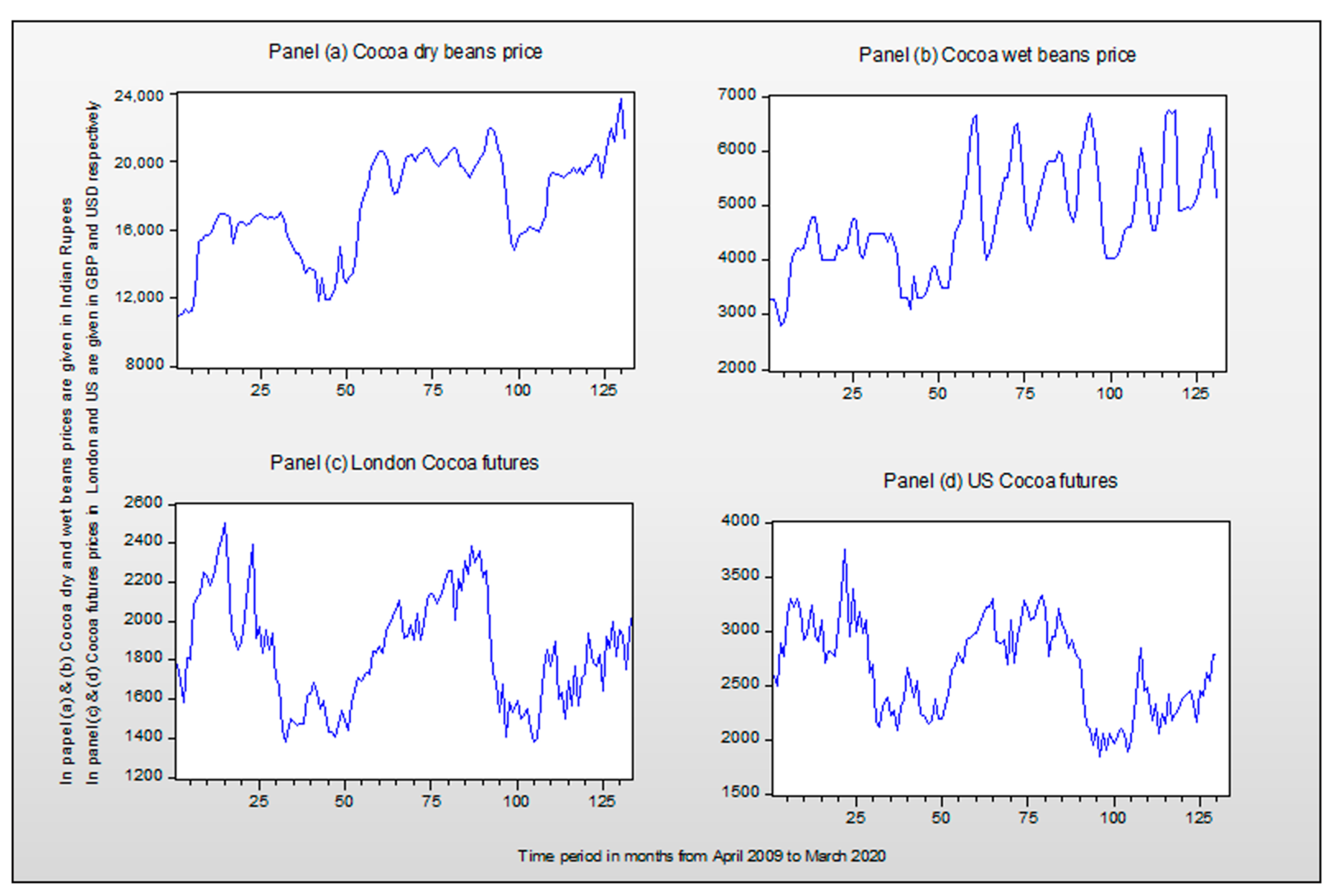
The study’s objective is to develop a price forecast for two varieties of Cocoa in India. Data for this time series study were collected from the office of The Central Arecanut and Cocoa Marketing and Processing Co-operative limited (CAMPCO). The monthly data were collected for the period starting from April 2009 to March 2020. For the same time period, the ICE US and London Cocoa futures prices were collected from the official website of investing.com. Two varieties of Cocoa beans are traded in the Karnataka state of India: Dry Cocoa beans and Wet Cocoa beans. In this study, we analyzed the price series of both varieties of Cocoa. The ARIMA and VAR models were developed for both of these series. From the data perspective in the time series analysis, the prerequisite is the stationarity of the series. If the series used for econometric analysis is not stationary, such analysis will give a spurious regression (Gujarati et al. 2009). To tackle such stationary issues, researchers can use integrated series with d order differences in the raw series (Kunst 2011). Many econometric experts (for example, Mills and Patterson (2009); Kunst (2011); Gujarati et al. (2009)) opined that correlograms of the series would give an initial clue on the stationarity of the series. However, formal hypothesis testing such as the Augmented Dickey–Fuller test is advised. Hence, in this study, correlograms and the Augmented Dickey–Fuller test are used to check the stationarity of the series.

Linear regression is a common tool used for forecasts. The general term of a bivariate linear regression model is shown in the Equation (1).

$$y_t=\alpha +\beta \left(x_t\right)+{\epsilon }_t$$

(1)

In this simple form of a linear regression equation, $y_t$ is the dependent variable, $x_t$ is the explanatory or independent variable, $\alpha$ and $\beta$ are the constants, and ${\epsilon }_{t }$ is the error of the model (Rawlings et al. 1998). The same model has been extended for multi-variate predictions; this model could be suitable when the researcher has more than one independent variable for the dependent variable of his interest. The general form of this multivariate regression model is shown in the Equation (2).

$$y_t=\alpha +{\beta }_1\left(x_{1t}\right)+{\beta }_2\left(x_{2t}\right)+\dots +{\beta }_n\left(x_{nt}\right)+{\epsilon }_t$$

(2)

In the second equation, we can observe multiple independent variables with names $x_1$, $x_2,$ and $x_n$ and their relationship factors ${\beta }_1$,${\beta }_2$, and ${\beta }_n$ with dependent variable $y_t$. The above two regression equations or methodology can be used only when the determinants of $y_t$ are measurable. In the short run, although explanatory variables are constant, the $y_t$ might vary due to market trends. In such situations, the application of univariate models such as Auto-Regressive (AR), Moving Average (MA), Auto Regressive Moving Average (ARMA), or Auto-Regressive Integrated Moving Average (ARIMA) would be most appropriate (Brooks 2008). These models’ very common pervasive characteristic is that the explanatory variables in all these models are the past values of the dependent series or its error terms (Stanton 2017). This is evident from the following third, fourth, and fifth equations.

$$y_t=\mu +{\beta }_{1yt-1}+{\beta }_{2yt-2}+\dots +{\beta }_{pyt-p}+u_t$$

(3)

$$y_t=\mu +u_t+{\theta }_{1ut-1}+{\theta }_{2ut-2}+\dots +{\theta }_{qut-q}$$

(4)

$$y_t=\mu +{\beta }_{1yt-1}+{\beta }_{2yt-2}+\dots +{\beta }_{pyt-p}+{\theta }_{1ut-1}+{\theta }_{2ut-2}+\dots +{\theta }_{qut-q}+u_t$$

(5)

Equations three, four, and five are the general form of the AR, MA, and ARMA process, where $y_t$ is the value of the dependent variable. In equations three, four, and five,$u_t$ denotes the white noise error term, where $p\wedge q$ denotes the optimal number of lags for the AR (p) and MA (q) process. AR model implies the present value of the dependent variable, y, depending on its past values. MA model implies that the current value of the dependent variable is the function of the present and the past values of a white noise error term (Chris Brooks 2014). Equation five shows the characteristics of the ARIMA model, where the current value of the dependent variable, y, is the function of its past values plus the blend of the present and past values of a white noise disturbance term (Brooks 2008). If the raw series is stationary at its base level, then the model applicable would be ARMA (p, q,); however, if the series is not stationary, then such series calls for integrated or differenced series to avoid spurious regression. Such differenced series would be used to identify the AR (p) and MA (q) terms for the ARMA model (Fabozzi et al. 2014). Hence, Box and Jenkins ARIMA modelling differs from ARMA, with additional terms ‘integrated’ and ‘I’ in the acronym.

The first half of Section 4 focuses on the identification of ‘p’, ‘q’, and ‘d’ parameters for the ARIMA model to forecast the monthly price of Cocoa. Parameter ‘d’ is the order of differencing to make the series stationary. Once the series becomes stationary, the graphical representation of the Auto Correlation Function (ACF) and Partial Auto Correlation Function (PACF) of the stationary series can be used to identify the ‘p’ and ‘q’ parameters (Meeker 2001). However, Brooks (2008) opined that interpreting ACF and PACF correlograms are not an easy task because these figures rarely produce simple patterns. Hence, it is advised to use information criteria statistics of the estimates to decide on the number of lags or parameters for the model. There are three popular information criteria recommended by many econometricians for optimal lag selection; they are, Akaike’s information criteria (AIC), Schwarz’s Bayesian information criteria (SBIC), and the Hannan–Quinn criterion (HQIC) (Agung 2009; Fabozzi et al. 2014; Mallikarjuna et al. 2019; Mills and Patterson 2009; Shmueli and Litchtendahl 2016). The ACF and PACF correlograms of the residuals of the estimates are used for the diagnostic checking (Gujarati et al. 2009). The following two hypotheses are developed and tested in this study.

H₀₁: 

The Dry Cocoa price series has a unit root.

H₀₂: 

The Wet Cocoa price series has a unit root.

H₀₃: 

The autocorrelation and partial autocorrelation values for residuals of the estimated model are not serially correlated.

Further, we develop the VAR model; the endogenous variables in the model are US Cocoa futures, London Cocoa futures, and Cocoa prices from India. The following equation shows the general form of the bivariate VAR model. Where (CP) in equation six is the Cocoa price, which is dependent on its own lagged values, lagged values of Cocoa futures price (CF), and $\left(u_{CPt}\right)$ is the white noise error term. CF in the seventh equation is the Cocoafuture price, which is dependent on its own lagged values and lagged values of Cocoa price (CP) and ($u_{CFt})$ is the white noise error term. However, we accommodate the above-mentioned three endogenous variables in the model.

$$C{P}_t={\beta }_{CP0}+{\beta }_{CP1}C{P}_{t-1}+\dots +{\beta }_{CPk}C{P}_{t-k}+{\propto }_{CPk}C{F}_{t-1}+\dots +{\alpha }_{CPk}C{F}_{t-k}+u_{CPt}$$

(6)

$$C{F}_t={\beta }_{CF0}+{\beta }_{CF1}C{F}_{t-1}+\dots +{\beta }_{CFk}C{F}_{t-k}+{\propto }_{CFk}C{P}_{t-1}+\dots +{\alpha }_{CFk}C{P}_{t-k}+u_{CFt}$$

(7)

4. Data Analysis and Interpretation

4.1. Test for Unit Root

The graphical representation of the time series will give an initial clue of the stationarity of the series. It is customary that the economic or commodity price time series shows an upward trend over a period of time. The price series of Dry Cocoa beans and the ICE Cocoa futures are not excluded from this fundamental theory; however, the Wet Cocoa beans series shows a mixed trend during the study period. The price of Cocoa in the years 2012 and 2013 dropped badly in the world market and the same is evident in the Indian market. The oil crisis and financial instability werethe major reasons for the volatility. In India, Cocoa is not produced as a major product; instead, it is grown as a mixed crop with Arecanut and Coconut plants. Hence, the impact of the price drop was not discussed much in the existing literature. Panel (a) in the first image shows the upward trend of the Dry Cocoa price series; this is a clear indication of a non-stationary or an auto-correlated time series. Hence, the raw series is integrated with first-order differences. Panel (b) shows the same upward trend, but the ADF test confirms that the Wet Cocoa price series is a stationary series. Panel (c) and (d) in the second image are the pictorial representations of the London Cocoa futures price series and US Cocoa futures price series; these graphs resemble the trend Dry Cocoa price series. However, a hypothesis testing using Augmented Dickey–Fuller test will confirm this formally.

Unit root test results are presented in

Table 1. Unit-root test results. Source: Authors processing.

Panel a: Cocoa and currency price series
Prices	t-Statistic	Test critical Values			p-Value
		1% Level	5% Level	10% Level
Dry Beans price series	−2.41	−3.48	−2.88	−2.58	0.14
Wet Beans price series	−4.90	−3.48	−2.88	−2.58	0.00
US Cocoa futures	−2.55	−3.48	−2.88	−2.58	0.11
London Cocoa futures	−2.89	−3.48	−2.88	−2.58	0.06
Panel b: Cocoa and currency return series
Returns	t-Statistic	Test critical Values			p-Value
		1% Level	5% Level	10% Level
Dry Beans price series	−9.38	−3.48	−2.88	−2.58	0.00
US Cocoa futures	−7.56	−3.48	−2.88	−2.58	0.00
London Cocoa futures	−6.96	−3.48	−2.88	−2.58	0.00
Panel c: P-P test for unit-root
Dry Beans price series	−2.44	−3.48	−2.88	−2.58	0.13
Wet Beans price series	−4.85	−3.48	−2.88	−2.58	0.00
Dry Beans price series	−8.75	−3.48	−2.88	−2.58	0.00

. As Figure 1 depicts, for the Dry Cocoa beans price series, there is not enough evidence to reject the null hypothesis. The probability value is more than 0.05 and the t statistics lie inside the cutoff point of −2.414 for all common significance levels. However, in the case of Wet Cocoa beans price series, the MacKinnon probability value is less than 0.05, and even the t values are outside the cut-off point of −4.897823 for all common significance levels. This confirms that the raw Dry Cocoa price series is serially correlated and the Wet Cocoa price series is a non-stationary time series. The Augmented Dickey–Fuller test for differenced Dry Cocoa beans price series is shown. The MacKinnon probability value of (0.00), which is less than 0.05, and the t statistic values for all levels of significance are in the rejection region. This rejects the null hypothesis, and now the differenced series is not serially correlated. The MacKinnon probability values of US Cocoa futures and London Cocoa futures confirm that the price series is non-stationary in its original form. The return series of US Cocoa futures and London Cocoa futures are free from autocorrelation with probability values of 0.00 and 0.00. The Phillips–Perron (P-P) test statistics for the price and return series of dry and wet Cocoa series are presented in panel (c) of Table 1; the results of this test are identical to the ADF tests.

The descriptive statistics for the price and return series of dry and wet Cocoa beans are presented in

Table 2. Descriptive statistics of dry and wet Cocoa beans price/return series.

	Panel a: Price Series		Panel a: Return Series
	Dry Cocoa Beans	Wet Cocoa Beans	Dry Cocoa Beans	Wet Cocoa Beans
Mean	17,484.82	4725.46	0.01	0.00
Maximum	23,709.48	6748.00	0.21	5.52
Minimum	10,932.00	19.76	−0.14	−5.83
Std. Dev.	2966.43	1061.47	0.05	0.71
Skewness	−0.41	−0.40	0.44	−0.68
Kurtosis	2.28	4.70	6.33	64.13
Jarque–Bera	6.49	19.28	64.62	20,409.24
Observations	131.00	131.00	130.00	130.00

Source: Authors computations.

. The mean returns of both the series are less than their respective standard deviations; this implies that the return series of dry and wet Cocoa beans are highly volatile. The negative skewness in the price and return series of wet Cocoa beans indicates the heavy losses or longer left tails in the series. High Kurtosis in the return series of wet Cocoa beans indicates the presence of fat tails in the series.

4.2. Box–JenkinsARIMA Model Identification

This paper aims to identify the AR (p), MA (q), and I (d) terms for the forecasting model. In these three terms, the I (d) term is already identified. The Dry Cocoa beans price series became stationary after the first order differencing; hence, the I (d) term for this model is process is I (1). However, the Wet Cocoa beans price series was stationary in its base level without integration or differencing; hence, the I (d) term for this model process is I (0) and the resulting model may become AR or MA or ARMA. Further to identify the AR and MA terms for the model ACF and PACF correlograms are used; however, Brooks (2008) mentioned that ACF and PACF correlograms will produce complicated graphs. Hence, these ACF and PACF correlograms can be used to identify only the tentative models. The information criteria of the estimates can be used to finally decide on the optimal lags for the model. Figure 2 and Figure 3 are the pictorial representation of ACF and PACF of differenced Dry Cocoa beans price series and Wet Cocoa beans price series.

In the last section, the Augmented Dickey–Fuller test and line plot graph confirmed that the differenced Dry Cocoa series is not stationary.

Table 3. Autocorrelation and partial autocorrelation values for differenced Dry Cocoa Beans price series.

Dry Cocoa Beans
Lag	Autocorrelation	Partial Autocorrelation	Prob
1	0.164	0.164	0.057
2	0.094	0.069	0.090
3	0.021	−0.005	0.181
4	−0.017	−0.027	0.296
5	0.054	0.062	0.378
6	−0.034	−0.050	0.484
7	0.104	0.112	0.429
8	−0.030	−0.062	0.523
9	−0.007	−0.005	0.623
10	−0.185	−0.195	0.279
11	0.015	0.100	0.355
12	0.013	0.001	0.434
13	0.002	0.019	0.516
14	−0.009	−0.053	0.594
15	−0.122	−0.083	0.496
16	−0.041	−0.035	0.551

Source: Authors computations using SPSS package.

above shows that the autocorrelation values are negligible and the correlation value dies off by the fourth lag. However, our focus here is to identify the tentative parameters for the AR and MA process of the ARIMA methodology. It is evident from the second Table that the auto-correlation values are not significant with a 95% confidence interval. Gujarati et al. (2009) stated that the identification of model parameters is an art, because different people may identify different parameters by looking at the ACF and PACF correlograms, which are similar, but not identical. Theoretically, rule of thumb is that if the initial lags of ACF have significant spikes and those spikes slowly decay, then that is the symptom of an Auto-Regressive (AR) process. It is an indication that the value $y_t$ is the function or its past values. Further, if the PACF is positive in its first lag and cuts off deeply, then again, that is the sign of an Auto Regressive (AR) process. Contradictorily if the ACF in the first lag is negative, such a series follows the Moving Average (MA) process.

The ACF in the first lag does not show significant spikes in the initial lags; moreover, the ACF decays immediately in the third or fourth lag. However, both the ACF and the PACF values are positive in the first lag for the differenced series. Further, as the first lag of ACF is not negative, adding value to the AR process makes sense. Very importantly, both ACF and PACF values in the first lags are just equal to or below the 95% confidence interval; further, the ACF and PACF values for all 15 lags are inside the 95% confidence interval. Graphical representation rarely gives precise AR and MA parameters (Chris Brooks 2014). Hence, the following tentative models are selected based on the above discussions. For tentative models (1, 1, 1), (0, 1, 1), and (1, 1, 0), regression coefficients will be estimated and, based on information criteria, an optimal model will be selected.

Interestingly, the Wet Cocoa beans price series proved to be a white noise series by the Augmented Dickey-Fuller test and line plot graph. However, the ACF and PACF values disprove the tested hypothesis. Table 3 shows that the autocorrelation values are not equal to zero until the sixteenth lag and the correlation values are gradually decreasing; this is the sign of a non-stationary series. The serially correlated series will produce nonsense coefficients and such spurious regressions would become evident by R² (the measure of goodness of fit) greater than the d value (Durbin–Watson) (Yule 1926; Granger and Newbold 1974). Hence, the first order differenced series is also analyzed; the ACF and PACF values of such differenced series exhibit the characteristics of a non-stationary series. For raw series of Wet Cocoa beans, the ACF in the inceptive lags manifests peaks and slowly decays. Panel (b) in the third image proclaims that the PACF in the first lag is positive and there is a drastic decline in the PACF pattern immediately from the second lag. Moreover, the ACF in the initial lags shows a prolonged decline, and these are all the characteristics of an AR process. Pragmatic approaches are to reckon the PACF cut-off point and select it as Auto-Regressive (AR) term for the model.

Likewise, the lag where ACF dies off will become the Moving Average (MA) term for the model. Gujarati et al. (2009) opined that during the AR and MA term identification process, researchers have to look for terms with possible minimum lags, and that the parsimony should be the key. With these rationales, tentative models (1, 1, 1), (1, 1, 2), (1, 1, 3), and (1, 1, 4) are identified raw Wet Cocoa beans price series. The ACF and PACF correlograms of the first-order differenced Wet Cocoa price series is shown in Panel (c) and (d) of the third figure. The Section 2 in Table 3 shows the Autocorrelation and Partial Autocorrelation values of the differenced series. The ACF value in the first lag is negative and the series values are not serially correlated, which indicates a Moving Average (MA) process. As the ACF cuts off in the first lag itself, the identified term for the MA process is one, tentative models (1, 1, 1), (2, 1, 1), (3, 1, 1), and (4, 1, 1) are carried for the estimation process. The ACF and PACF estimates for the price and return series of Wet Cocoa beans is presented in

Table 4. ACF and PACF values for Raw and Differenced Wet Cocoa Beans price series.

	Wet Cocoa Beans			D. Wet Cocoa Beans
Lag	Autocorrelation	Partial Autocorrelation	Prob	Autocorrelation	Partial Autocorrelation	Prob
1	0.695	0.695	0.000	−0.488	−0.488	0.000
2	0.549	0.128	0.000	0.002	−0.310	0.000
3	0.389	−0.065	0.000	−0.004	−0.223	0.000
4	0.261	−0.049	0.000	−0.019	−0.198	0.000
5	0.221	0.092	0.000	0.007	−0.168	0.000
6	0.194	0.050	0.000	0.005	−0.138	0.000
7	0.180	0.019	0.000	−0.002	−0.120	0.000
8	0.199	0.073	0.000	0.010	−0.090	0.000
9	0.208	0.051	0.000	−0.009	−0.082	0.000
10	0.247	0.098	0.000	−0.012	−0.095	0.000
11	0.298	0.116	0.000	0.004	−0.097	0.001
12	0.329	0.075	0.000	0.001	−0.095	0.001
13	0.308	−0.027	0.000	0.008	−0.080	0.002
14	0.237	−0.082	0.000	0.006	−0.058	0.004
15	0.147	−0.074	0.000	−0.004	−0.047	0.006
16	0.081	−0.023	0.000	−0.008	−0.052	0.010

Source: Authors computations using SPSS package.

.

5. Estimation

Using the E Views-11 student version package, coefficients are estimated for all the identified tentative models. Customarily, the estimates output will produce coefficients along with some information criteria and goodness-of-fit statistics. Researchers often use the Akaike information criterion (AIC) and Schwarz criterion (SBIC) along with the regression coefficients, volatility, and adjusted R² to resolve the ambiguity of optimal AR and MA terms for an ARIMA model. In addition to these parameters, R² and Durbin—Watson statistics are also considered to measure the non-stationary series’ impact and avoid spurious regression.

From

Table 5. Summary of ARIMA estimation output for differenced Dry Cocoa Beans Price.

Differenced Dry Cocoa Beans Price	(1, 1, 1)	(0, 1, 1)	(1, 1, 0)
Number of Significant Coefficients	0	1	1
Sigma square	0.00232	0.00234	0.00233
Adjusted, R2	0.0094	0.0095	0.0135
AIC	−3.1666	−3.1742	−3.1783
SBIC	−3.0788	−3.1084	−3.1125
R2	0.0322	0.0247	0.0287
Durbin–Watson Statistic	1.9416	1.9116	1.9585

Source: Authors processing using EViews 11 package.

, it is understandable that the regression coefficients tentative model (1, 1, 1) is not statistically significant. Hence, model (1, 1, 1) can be filtered, and the other two models are carried forward for further analysis with other statistical values. Sigma square is the measure of volatility; a model with a lower sigma square is preferred, and likewise, a model with the lowest Akaike information criterion (AIC) and Schwarz criterion (SBIC) is considered as a better model (Gujarati et al. 2009). Further adjusted R² is the measure of goodness of fit; customarily, the model with the highest R² is considered as the better model. With these criteria, model (1, 1, 0) is considered an appropriate model because the volatility, AIC, and SBIC values of this model are less compared to model (0, 1, 1). Even the adjusted (R²) favors the model (1, 1, 0). There is no symptom of autocorrelation in the analyzed series because the R² value is less than Durbin–Watson d statistic value. Moreover, the Durbin–Watson value closes to two indicates a non-stationary series; hence, the estimated coefficients are not spurious.

The first exciting discussion in this section is about the contradictory discussion from the identification section about the stationarity of the raw Wet Cocoa beans price series. The estimates for the tentative models of the raw Wet Cocoa beans price series are presented in

Table 6. Summary of ARIMA estimation output for Raw Wet Cocoa Beans Price series.

Raw Cocoa Beans Price	(1, 1, 1)	(1, 1, 2)	(1, 1, 3)	(1, 1, 4)
Number of Significant Coefficients’	2	2	1	1
Volatility	564,350.700	560,963.800	573,409.200	570,601.800
Adjusted, R2	0.489	0.492	0.481	0.484
AIC	16.147	16.142	16.163	16.158
SBIC	16.235	16.229	16.250	16.246
R2	0.501	0.504	0.493	0.496
Durbin–Watson Statistic	2.013	2.043	2.172	2.226

Source: Authors processing using EViews package.

. The R² and the Durbin–Watson statistic are brought here in this Table to check whether the model has produced spurious regression because of serially correlated series. The ACF and PACF correlograms depicted a graph identical to a non-stationary series. However, the R² and Durbin–Watson statistics in Table 6 favor the Augmented Dickey–Fuller test result. Durbin–Watson statistic values are very close to two and the R² values are less than Durbin–Watson d values for all the estimations. Hence, the raw Wet Cocoa price series is a non-stationary series and the estimates are not spurious, so it is not necessary to estimate the coefficients for differenced Wet Cocoa price series. From other statistics from Table 6, models (1, 1, 3) and (1, 1, 4) can be dropped easily because both AR and MA have statistically significant coefficients; for the other two models, both AR and MA have statistically significant coefficients. The volatility model (1, 1, 1) estimate is greater than the volatility of the model (1, 1, 2) estimate.

Similarly, the AIC and the SBIC values favor the model (1, 1, 2). The adjusted R² value of model (1, 1, 2) is greater than the other model in the race. Hence, the ARIMA optimal models based on information criteria are model (1, 1, 0) for Dry Cocoa beans price and model (1, 1, 2) for Wet Cocoa price. Diagnostic checking with the help of residuals of the estimates is advised by many econometricians (Gujarati et al. 2009; Brooks 2008).

6. Diagnostic Checking

Whether the estimated model is good enough for prediction is the obvious question that arises after the model estimation. If the model is not suitable for predictions, such model parameters may have to be revised by repeating all the procedures starting from the introduction till the diagnostic check. To perform the diagnostic check, the developers of the methodology, Box and Jenkins, advised residual diagnostic and over fitting methods. Moreover, to measure the goodness of fit for the estimated ARIMA model, many econometricians have suggested examining the ACF and PACF correlograms of the residuals (Brooks 2008; Meeker 2001; Gujarati et al. 2009). The aim is to construct a parsimonious or over fitted model, which is not advised because such a model may result in high standard errors for coefficients. The theory of the parsimonious model was taken care of in the identification section and now it is essential to examine the correlograms to check whether the residuals are serially correlated.

The correlograms of ACF and PACF in Figure 4 confirm that the residuals not serially correlated, because both ACF and PACF correlograms are simply flat. For all the lags, the ACF and PACF are within the 95 percent confidence interval.

Table 7. Auto correlation and Partial autocorrelation values for residuals of models(1, 1, 0) and (1, 1, 2).

Residuals of D. Dry Cocoa Price Series Model (1, 1, 0) Estimates				Residuals of Wet Cocoa Price Series Model (1, 1, 2) Estimates
AC	PAC	Q-Stat	Prob	AC	PAC	Q-Stat	Prob
−0.013	−0.013	0.0223		−0.033	−0.033	0.1463
0.065	0.065	0.5893	0.443	−0.014	−0.015	0.1734
0.004	0.005	0.5912	0.744	0.056	0.055	0.6088	0.435
−0.028	−0.033	0.7017	0.873	−0.053	−0.05	0.9998	0.607
0.065	0.064	1.2772	0.865	0.027	0.025	1.1005	0.777
−0.068	−0.063	1.9186	0.86	0.031	0.028	1.2324	0.873
0.117	0.11	3.8577	0.696	0.001	0.01	1.2326	0.942
−0.045	−0.038	4.1413	0.763	0.054	0.05	1.6411	0.95
0.032	0.023	4.29	0.83	−0.002	0.001	1.6416	0.977
−0.2	−0.21	10.066	0.345	0.017	0.02	1.6836	0.989
0.047	0.066	10.385	0.407	0.086	0.082	2.7638	0.973
0.009	0.006	10.396	0.495	0.11	0.122	4.5592	0.919
0.003	0.029	10.397	0.581	0.136	0.148	7.3286	0.772
0.011	−0.032	10.417	0.66	0.074	0.087	8.1411	0.774
−0.119	−0.082	12.55	0.562	−0.014	−0.002	8.1726	0.832
−0.016	−0.06	12.591	0.634	−0.049	−0.057	8.5437	0.859
−0.029	0.043	12.716	0.693	−0.018	−0.029	8.5945	0.898
0.024	0.005	12.808	0.749	0.007	−0.006	8.6015	0.929
−0.019	−0.01	12.863	0.8	−0.002	−0.022	8.6024	0.952
0.012	−0.033	12.884	0.844	−0.014	−0.039	8.6348	0.968
0.036	0.057	13.09	0.873	0.036	0.014	8.8452	0.976
−0.073	−0.062	13.949	0.872	0.096	0.088	10.335	0.962
−0.008	−0.001	13.96	0.903	0.083	0.082	11.46	0.953
−0.058	−0.063	14.517	0.911	0.089	0.073	12.757	0.94

Source: Authors computations using E Views package.

shows that auto correlation (AC)and partial auto correlation (PAC) values are very minor and the probability values with a 95 percent confidence interval prove that the residuals series for the model (1, 1, 0) and (1, 1, 2) are not serially correlated. This confirms that the estimated models have captured all the pieces of information and there is no need to revise the model parameters. Hence, the ARIMA (1, 1, 0) is the optimal model to predict the monthly prices of Dry Cocoa beans; likewise, model (1, 1, 2) is an optimal model to predict the monthly price of Wet Cocoa beans.

7. VAR Model

The vector auto regressive methodology begins with identifying the optimal lag order. The Akaike information criterion (AIC), Schwarz information criterion (SC), and Hannan–Quinn information criterion (HQ) are used to decide on the optimal lag order for the VAR model. The AIC, SC, and HQ values are presented in

Table 8. VAR lag order selection criteria.

Lag	AIC	SC	HQ
0	8.43	8.52	8.47
1	5.25	5.71 *	5.44 *
2	5.14 *	5.96	5.47
3	5.29	6.49	5.78
4	5.39	6.96	6.03

Source: Authors computations using E Views package. Optimum number of lag is indicated by *.

. The AIC identified lag order 2 as the optimal lag, and SC– and HQ (majority) criterions notified lag order 1 as the optimal lag. Hence, lag order 1 is considered as the optimal lag order for the proposed VAR.

This multivariate VAR has four endogenous variables and the optimal lag order is one. Hence, each equation in the model will have (4 $\times$ 1 + exogenous intercept c = 1) regressors.

Table 9. VAR (1) regression estimations.

Other Variable	Dry Cocoa Beans	Prob.	Other Variable	Wet Cocoa Beans	Prob
US Cocoa futures (−1)	0.108	0.04	US Cocoa futures (−1)	−0.047	0.439
	0.053			0.088
	[2.033]			[−0.534]
Dry Cocoa Beans (−1)	0.149	0.50	Dry Cocoa Beans (−1)	0.128	0.57
	0.085			0.167
	[1.747]			[0.769]
London Cocoa futures (−1)	0.171	0.0	London Cocoa futures (−1)	0.112	0.747
	0.058			0.098
	[2.867]			[1.137]
Wet Cocoa Beans (−1)	−0.002	0.09	Wet Cocoa Beans (−1)	0.379	0
	−0.032			0.097
	[−2.26]			[3.919]
C	0.0049	0.01	C	0.002	0.88
	0.004			0.007
	[1.219]			0.268

Source: Authors computations using E Views package.

presents the regression estimate coefficients with standard error, t-statistics, and probability values.

With four endogenous variables, this VAR (1) model has estimated 25 coefficients, 10 of 25 are presented in Table 8. Our interest is to examine the linkage between the Indian Cocoa market with ICE Cocoa futures. Hence, only the estimates for the Wet and Dry Cocoa series are presented in the above table. The estimates highlighted in bold are statistically significant with a 95% confidence level. The coefficients with the first lag of US Cocoa futures, London Cocoa futures, and Wet Cocoa price are significant for the Dry Cocoa price series. This confirms that the ICE traded US and London Cocoa futures price will influence the price of Dry Cocoa in India. This finding is similar to the findings of (Jumah and Kunst 2001) and (Sahay et al. 2002). They found the linkage of the currencies, US Dollar and Pound Sterling, with Cocoa prices in the international market. They justify that the trade of US Cocoa futures and London Cocoa futures in the ICE platform are the primary reasons for such a linkage. However, the Wet Cocoa beans price in India is not affected by the ICE Cocoa futures. The first lag of its own series is statistically significant for Wet Cocoa prices. The changes in the international Cocoa price will be corrected in the Indian Dry Cocoa market. The equation given by the VAR system to forecast the price of Cocoa prices in India is shown in Equation (8)

$$\begin{array}{cc}\hfill DryBeansPrice& =C\left(6\right)\times USCococFutures\left(-1\right)+C\left(7\right)\times DryBeansPrice\left(-1\right)\hfill \\ & +C\left(8\right)\times WetBeansPrice\left(-1\right)+C\left(9\right)\times LondonCocoaFutures\left(-1\right)+C\left(10\right)\hfill \end{array}$$

(8)

In Equation (8) coefficients C(7), C(8), and C(10) are not statistically significant. Hence, Equation (8) is represented as Equation (9) by substituting the actual significant coefficients.

$$DryBeansPrice=0.108\times USCococFutures\left(-1\right)+0.171\times LondonCocoaFutures\left(-1\right)$$

(9)

To understand the goodness of fit of the estimated VAR equations, the fitness summary is presented in

Table 10. Fitness summary for the estimated VAR equations.

Statistic	US Cocoa Futures	Dry Cocoa Beans	London Cocoa Futures	Wet Cocoa Beans
R-squared	0.19	0.14	0.74	0.84
Adj. R-squared	0.16	0.11	0.73	0.84
S.E. equation	0.07	0.05	0.04	393.17
Durbin–Watson stat	1.87	2.08	2.20	1.60
Mean dependent	0.00	0.01	0.00	4783.27
S.D. dependent	0.08	0.05	0.07	970.46

. The R² in Table 5 indicates the goodness of fit; this value is 14% for dry Cocoa beans and 84% for wet Cocoa beans. These statistical values imply the proportion of variance in dry and wet Cocoa returns that can be explained by our coefficients. The Durbin–Watson statistic was used to test whether the residual series of the estimated VAR models were serially correlated, and the test value of dry Cocoa beans was close to two, which indicates that the residuals in the series were free from autocorrelation. Hence, the estimated model for dry Cocoa beans is a good fit; this model can be used for the short-term prediction of dry Cocoa beans in India.

The response of dry Cocoa beans returns to a unit shock in the US and London Cocoa futures is shown in Figure 5. The red lines are 95% confidence intervals and the blue line indicates the impulse response function. The response of dry Cocoa beans returns for the US Cocoa futures shock are sharp and positive at the beginning, stabilize and sharp decrease until the fifth lag, and then they die off after the sixth lag. The response for London Cocoa futures shock is also sharp positive in the beginning, followed by a steady decline till the fifth lag, and then it dies off thereafter.

The market-based tools such as futures or options will help in price discovery and price locking. The price of any commodity is the function of demand and supply for that commodity in the market. Price discovery is the primary function of market-based risk management tools such as futures and options (Chng 2004). In the futures market, as a commodity will be traded for future delivery, and as the trading happens from all parts of the nation, the traders perform all the possible analyses before they lock the price. Hence, the futures quote can become a good price forecast for any underlying circumstance. A study by Malhotra and Corelli (2021) proved that in the EURO/USD futures market, regular futures contributes 65% to price discovery. The e-auction helps in the price discovery of Cardamom in the Indian Market (Vijayakumar 2021).

In the absence of such predictions and hedging tools, the econometric prediction models will help in price risk management. Forecasting the price for a commodity is an integral part of price risk management. The Box–Jenkins ARIMA model assumes that the future values are the functions of past data; in particular, this methodology uses past terms of AR and MA to predict the future prices. This is proved by the empirical studies of (Fattah et al. 2018; Mishra et al. 2019). Many studies have appeared so far concerning the application of time series models to develop the price prediction models for different agricultural commodities. The same is discussed in the literature review section of this study. If the price determinant variables are available, in such cases, multivariate models can be applied to understand the linkage between two or many markets and to develop the price prediction models. This study has developed a univariate ARIMA model and a multivariate model VAR to forecast the price of Wet and Dry Cocoa beans in India. This study can be extended using multivariate time series models, and alternative price risk management strategies can be developed. As the direct futures are not available for commodity cocoa, cross hedges with other related futures can be examined.

8. Conclusions

The volatile business and agricultural market demand proper price risk management strategies. In this context, this study has developed two ARIMA models and one VAR model to predict the monthly prices for two varieties of Cocoa using Box and Jenkins methodology. Based on the Akaike information criterion (AIC) and Schwarz criterion (SBIC), volatility, and adjusted R², the optimal AR and MA terms are identified for the models. Based on the above criteria, the models selected are ARIMA (1, 1, 0) and ARIMA (1, 1, 2) for Dry Cocoa price and Wet Cocoa price, respectively. The correlograms of the residuals proved that the model is fit to use for prediction. The VAR (1) system produced significant coefficients only for Dry Cocoa beans. The VAR system proved that the US and London Cocoa Futures traded on the ICE platform are the price determinants of Dry Cocoa beans in the Indian market. Jayasekhar and Ndung (2018) stated that the Cocoa price in India is the function of price in the world market; this is evident from the developed VAR model.

This study will contribute to the existing literature on price risk management for commodity Cocoa in India. The models developed can be used by the Cocoa trading entities, growers, industrial users, and government authorities for timely planning and to take managerial decisions. As Cocoa futures are not traded in India, the cooperatives, traders, and manufacturers can trade with futures of ICE. The cooperatives and authorities can suggest the use of ICE futures to hedge the price risk of Cacao in India. The developed models help to discover the price of commodity Cocoa, which helps the farmer to decide on the selling decision and traders and industrial buyers on the buying decision. If one can anticipate the price, then one can decide on the buy or sell decision based on the predicted future price. This, in turn, helps the stakeholders to manage the price risk in the absence of derivative products such as futures and options.

References

1. Abdullah, Lazim. 2012. ARIMA Model for Gold Bullion Coin Selling Prices Forecasting. International Journal of Advances in Applied Sciences 1: 153–58. [Google Scholar] [CrossRef]
2. Abonazel, Mohamed Reda, and Abd-elftah Ahmed Ibrahim. 2019. Forecasting Egyptian GDP Using ARIMA Models. Reports on Economics and Finance 5: 35–47. [Google Scholar] [CrossRef]
3. Adebiyi, Ayodele A., Adewumi Aderemi, and Ayo Charles. 2014. Stock Price Prediction Using the ARIMA Model. Paper presented at International Conference on Computer Modelling and Simulation, Cambridge, UK, March 26–28; pp. 105–11. [Google Scholar] [CrossRef] [Green Version]
4. Agung, Gusti Ngurah. 2009. Time Series Data Analysis Using Eviews. Hoboken: John Wiley & Sons. [Google Scholar]
5. Akgül, Isil, Bildirici Melike, and Selin Özdemir. 2015. Evaluating the Nonlinear Linkage between Gold Prices and Stock Market Index Using Markov-Switching Bayesian VAR Models. Procedia—Social and Behavioral Sciences 210: 408–15. [Google Scholar] [CrossRef] [Green Version]
6. Bataa, Erdenebat, Denise R. Osborn, and Marianne Sensier. 2018. China’s increasing global influence: Changes in international growth linkages. Economic Modelling 74: 194–206. [Google Scholar] [CrossRef]
7. Brooks, Chris. 2008. Econometrics Introduction, 2nd ed. New York: Cambridge University Press, Available online: www.cambridge.org/9780521873062 (accessed on 29 April 2018).
8. Brown, Oli, Alec Crawford, and Jason Gibson. 2008. Boom or Bust: How Commodity Price Volatility Impedes Poverty Reduction, and What to Do about It. Manitoba: International Institute for Sustainable Development, Available online: http://www.iisd.org/ (accessed on 12 January 2022).
9. Buhl, Hans Ulrich, Sofie Strauß, and Julia Wiesent. 2011. The impact of commodity price risk management on the profits of a company. Resources Policy 36: 346–53. [Google Scholar] [CrossRef]
10. Chin, Lawrence, and Gang Zhi Fan. 2005. Autoregressive analysis of Singapore’ s private residential prices. Emarald Insights 23: 257–70. [Google Scholar] [CrossRef]
11. Chloe, Taylor. 2021. “It’s difficult to feed our families”: Volatile cocoa prices are pushing West African farmers further into poverty. Cnbc 141. [Google Scholar]
12. Chng, Michael. 2004. A model of price discovery and market design: Theory and empirical evidence. Journal of Futures Markets 24: 1107–46. [Google Scholar] [CrossRef]
13. Chris Brooks. 2014. Stata Guide to Accompany Introductory Econometrics for Finance. Cambridge: Cambridge University Press. [Google Scholar]
14. Cortez, C. A. Tapai, S. Saydam, J. Coulton, and C. Sammut. 2018. Alternative techniques for forecasting mineral commodity prices. International Journal of Mining Science and Technology 28: 309–22. [Google Scholar] [CrossRef]
15. Darekar, Ashwini, and A.Amarender Reddy. 2017. Cotton Price Forecasting in Major Producing States. Economic Affairs 62: 373–78. [Google Scholar] [CrossRef]
16. Directorate of Cashewnut and Cocoa Development. 2020a. Area, Production and Productivity of Cocoa, Department of Agriculture, Cooperation and Farmers Welfare, Ministry of Agriculture and Farmers Welfare, Government of India. New Delhi: Directorate of Cashewnut and Cocoa Development. [Google Scholar]
17. Directorate of Cashewnut and Cocoa Development. 2020b. Export and Import of Cocoa and Cocoa preparations, Department of Agriculture, Cooperation and Farmers Welfare, Ministry of Agriculture and Farmers Welfare. New Delhi: Directorate of Cashewnut and Cocoa Development. [Google Scholar]
18. Directorate of Cashewnut and Cocoa Development. 2020c. Production scenario of Cocoa, Department of Agriculture, Cooperation and Farmers Welfare, Ministry of Agriculture and Farmers Welfare. New Delhi: Directorate of Cashewnut and Cocoa Development. [Google Scholar]
19. Fabozzi, Frank, Sergio Focardi, Svetlozer.T. Rachev, and Bala Arshanapalli. 2014. The Basics of Financial Econometrics. Hoboken: John Wiley & Sons. [Google Scholar]
20. FAO, IFAD, IMF, OECD, UNCTAD, WFP, The World Bank, The WTO, and The UN.HLTF. 2011. Price Volatility in Food and Agricultural Markets: Policy Responses, Risk Management. Roma: FAO. [Google Scholar]
21. Farooqi, Ahmad. 2014. ARIMA Model Building and Forecasting on Imports and Exports of Pakistan. Pak.j.stat.oper.res 10: 157–68. [Google Scholar] [CrossRef] [Green Version]
22. Fattah, Jamal, Latifa Ezzine, Zineb Aman, Haj El Moussami, and Abdeslam Lachhab. 2018. Forecasting of demand using ARIMA model. International Journal of Engineering Business Management 10: 1–9. [Google Scholar] [CrossRef] [Green Version]
23. Fauziah Widayat, Dessanty, Ratya Anindita, and Putri Budi Setyowati. 2019. The influence of cocoa price volatility (Theobroma cacao L.) to cocoa exports in indonesia. Agricultural Social Economic Journal 19: 117–24. [Google Scholar] [CrossRef] [Green Version]
24. Gaudenzi, Barbara, George A Zsidisin, Janet Hartley, and Lutz Kaufmann. 2018. An exploration of factors influencing the choice of commodity price risk mitigation strategies. Journal of Purchasing and Supply Management 24: 218–37. [Google Scholar] [CrossRef]
25. Granger and Newbold. 1974. Spurious regressions in econometrics. Journal of Econometrics 2: 111–20. [Google Scholar] [CrossRef] [Green Version]
26. Gujarati, Damodar N., Dawn C Porter, and Sangeetha Gunasekar. 2009. Basic Econometrics, 5th ed. New York: Mc Graw Hill Education. [Google Scholar]
27. Hossain, Zakir Md, Quazi Abdus Samad, and Zulficar Md Ali. 2006. ARIMA model and forecasting with three types of pulse prices in Bangladesh: A case study. International Journal of Social Economics 33: 344–53. [Google Scholar] [CrossRef]
28. Hubballi, Venkatesh N. 2015. Cocoa Development in India. New Delhi: Directorate of Cashewnut and Cocoa Development Ministry of Agriculture and Farmers Welfare, Government of India, pp. 23–29. [Google Scholar]
29. Janchum, Nontasak, Sangrawee Witoonpan, and Chalita Cheewaviriyanon. 2017. Price risk management strategies in commodity Markets. Journal of Management Sciences 4: 1–30. [Google Scholar]
30. Jayasekhar, S., and Isaac Ndung. 2018. Review of economic history of cocoa with special reference to India. Journal of Plantation Crops 46: 133–38. [Google Scholar] [CrossRef] [Green Version]
31. Jumah, Adusei, and Robert M. Kunst. 2001. The effects of dollar/sterling exchange rate volatility on futures markets for coffee and cocoa. European Review of Agricultural Economics 28: 307–28. [Google Scholar] [CrossRef] [Green Version]
32. Kumar, Abhaya K., Pinto Prakash, Hawaldar Iqbal Thonse, Spulbar Cristi, Birau Ramona, and Minea Loredana. 2021a. Forecasting Areca Nut Market Prices Using The Arima Model: A Case Study of India. Annals of the “Constantin Brâncuşi” University of Târgu Jiu, Economy Series. pp. 4–18. Available online: https://www.utgjiu.ro/revista/ec/pdf/2021-02/01_Kumar.pdf (accessed on 12 January 2022).
33. Kumar, Abhaya, Prakash Pinto, Iqbal Thonse Hawaldar, Cristi Marcel Spulbar, and Felicia Ramona Birau. 2021b. Crude oil futures to manage the price risk of natural rubber: Empirical evidence from India. Agricultural Economics—Czech 67: 423–34. [Google Scholar] [CrossRef]
34. Kunst, Robert. 2011. Applied Time Series Analysis—Part I. Vienna: University of Vienna and Institute for Advanced Studies Vienna. [Google Scholar]
35. Aidenvironment and Sustainable Food Lab. 2018. Pricing Mechanisms in the Cocoa Sector: Options to Reduce Price Volatility and Promote Farmer Value Capture. Hartland: Aidenvironment and Sustainable Food Lab. [Google Scholar]
36. Malhotra, Jatin, and Angelo Corelli. 2021. The relative informativeness of regular and e-mini euro/dollar futures contracts and the role of trader types. Risks 9: 111. [Google Scholar] [CrossRef]
37. Mallikarjuna, H. B., Anupriya Paul, Ajit Paul, Ashish S. Noel, and M. Sudheendra. 2019. Forecasting of Black Pepper Price in Karnataka State: An Application of ARIMA and ARCH Models. International Journal of Current Microbiology and Applied Sciences 8: 1486–96. [Google Scholar] [CrossRef]
38. Maurice, Noemie Eliana, and Junior Davis. 2011. Unraveling the Underlying Causes of Price Volatility in World Coffee and Cocoa Commodity Markets. Available online: https://mpra.ub.uni-muenchen.de/43813/ (accessed on 6 August 2020).
39. Meeker, William Q. 2001. Graphical Tools for Exploring and Analyzing Data from ARIMA Time Series Models. Ames: Iowa State University. [Google Scholar]
40. Mills, Terence C., and Kerry Patterson. 2009. Palgrave Handbook of Econometrics. Edited by Terence C. Mills and Kerry Patterson. London: Palgrave Macmillan. [Google Scholar]
41. Mishra, Manoj Kumar, B. V. S. Sisodia, and V. N. Rai. 2019. Forecasting technique of price of potato of Uttar Pradesh. Journal of Pharmacognosy and Phytochemistry 8: 60–62. [Google Scholar]
42. Mondal, Prapanna, Labani Shit, and Saptarsi Goswami. 2014. Study of Effectiveness of Time Series Modeling (ARIMA) in Forecasting Stock prices. International Journal of Computer Science, Engineering and Applications 4: 13–29. [Google Scholar] [CrossRef]
43. Nochai, Rangsan, and Nochai TItida. 2006. Arima model for forecasting oil. In Regional Conference on Mathematics, Statistics and Applications. Penang: University Sains Malaysis, pp. 1–7. [Google Scholar]
44. Oomes, Nienke, and Bert Tieben. 2016. Market Concentration and Price Formation in the Global Cocoa Value Chain, Seo Amsterdam Economics. The Hague: Ministry of Foreign Affairs. [Google Scholar]
45. Pipitone, Laurent. 2019. United Nations Conference on Trade and Development. In The Stae and Future of the Cocoa & Coffee Markets. Geneva: Routledge. [Google Scholar]
46. Qaiser Gillani, Durdana, Syed A. S. Gillani, Muhammad Z. Naeem, Cristi Spulbar, Elizabeth Coker-Farrell, Abdullah Ejaz, and Ramona Birau. 2021. The Nexus between Sustainable Economic Development and Government Health Expenditure in Asian Countries Based on Ecological Footprint Consumption. Sustainability 13: 6824. [Google Scholar] [CrossRef]
47. Radhika, Jayasekhar, and Muralidharan Amarnath. 2008. Seminar on Strategies for Enhancing Productivity of Cocoa. In Spatial Price Integration of Regional Cocoa Markets in India and with World Market: A Co-Integration Approach. Kasaragod: Central Plantation Crops Research Institute, pp. 165–70. [Google Scholar]
48. Rawlings, John O., Sastry G. Pantula, and David A. Dickey. 1998. Applied Regression Analysis: A Research Tool, 2nd ed. Berlin/Heidelberg: Springer Texts in Statistics. [Google Scholar]
49. Sahay, Ratna, Luis Céspedes, and Paul Cashin. 2002. Keynes, Cocoa, and Copper: In Search of Commodity Currencies. IMF Working Papers. p. 1. Available online: https://papers.ssrn.com/sol3/papers.cfm?abstract_id=880914 (accessed on 28 January 2022).
50. Sekhar, C. S. C. 2004. Agricultural Price Volatility in International and Indian Markets. Economic and Political Weekly 39: 4729–36. Available online: http://www.jstor.org/stable/4415712 (accessed on 12 January 2022).
51. Shil, Sandip, G. C. Acharya, C. T. Jose, K. Muralidharan, A. K. Sit, and George V. Thomas. 2013. Forecasting of arecanut market price in north eastern India: ARIMA modelling approach. Journal of Plantation Crops 41: 330–37. [Google Scholar]
52. Shmueli, Galit, and Kenneth C. Litchtendahl. 2016. Practical Time Series Forecasting with R, 2nd ed. Green Cove Springs: Axelrod Schnall. [Google Scholar]
53. Singh, Amanjot, and Manjith Singh. 2016. Inter-linkages and causal relationships between US and BRIC equity markets: An empirical investigation. Arab Economic and Business Journal 11: 115–45. [Google Scholar] [CrossRef]
54. Stanton, Jeffrey M. 2017. Galton, Pearson, and the Peas: A Brief History of Linear Regression for Statistics Instructors Galton, Pearson, and the Peas: A Brief History of Linear Regression for Statistics Instructors. Journal of Statistics Education 2017: 9. [Google Scholar] [CrossRef]
55. Sukiyono, Ketut, Musriyadi Nabiu, Bambang Sumantri, R. R. Novanda, Nyayu Neti Arianti, M. Zulkanain Yuliarso, Redy Badrudin, M. Mustopa Romdhon, and H. Mustamam. 2018. Selecting an Accurate Cacao Price Forecasting Model. Journal of Physics: Conference Series 1114: 1–6. [Google Scholar] [CrossRef]
56. Taghizadeh-Hesary, Farhad, Ehsan Rasoulinezhad, and Naoyuki Yoshino. 2019. Energy and Food Security: Linkages through Price Volatility. Energy Policy 128: 796–806. [Google Scholar] [CrossRef]
57. Tröster, Bernhard, Cornelia Staritz, Jan Grumiller, and Felix Maile. 2019. Commodity Dependence, Global Commodity Chains, Price Volatility and Financialisation: Price-Setting and Stabilisation in the Cocoa Sectors in Côte d’ Ivoire and Ghana. Vienna: ÖFSE. [Google Scholar]
58. Tse, Raymond Y. C. 1997. An application of the ARIMA model to real-estate prices in Hong Kong. Journal of Property Finance 8: 152–63. [Google Scholar] [CrossRef] [Green Version]
59. Tumala, Mohammed M., Afees A. Salisu, Ngozi V. Atoi, and Baba N. Yaaba. 2021. International monetary policy spillovers to emerging economies in Sub-Saharan Africa: A global VAR analysis. Scientific African 14: e00976. [Google Scholar] [CrossRef]
60. Vijayakumar, A. N. 2021. Price discovery and market efficiency of cardamom in India. Vilakshan—XIMB Journal of Management. ahead-of-print. [Google Scholar] [CrossRef]
61. Yousaf, Imran, and Shoaib Ali. 2020. The COVID-19 outbreak and high frequency information transmission between major cryptocurrencies: Evidence from the VAR-DCC-GARCH approach. Borsa Istanbul Review 20: S1–S10. [Google Scholar] [CrossRef]
62. Yule, G. Udny. 1926. Why do we sometimes get nonsense-correlations between time-series ?—A study in sampling and the nature of time-series. Royal Statistical Society 89: 1–63. [Google Scholar] [CrossRef]
Figure 1. Time plot of Cocoa spot price series and ICE Cocoa futures price series.
Risks 10 00115 g001
Figure 2. ACF and PACF Correlograms of Differenced Dry Cocoa price series. Source: Authors processing using SPSS package.
Risks 10 00115 g002
Figure 3. (a) The ACF correlograms for the raw Wet Cocoa beans price series; (b) The PACF correlograms for the raw Wet Cocoa beans price series; (c) The ACF correlograms for the differenced Wet Cocoa beans price series; (d) The PACF correlograms for the differenced Wet Cocoa beans price series.
Risks 10 00115 g003
Figure 4. ACF and PACF correlograms for the residuals of (1, 1, 0) and (1, 1, 2) models. Source: Authors processing using EViews package.
Risks 10 00115 g004
Figure 5. Impulse response of dry Cocoa beans returns to ICE traded Cocoa futures. The red line is 95% confidence interval and the blue line is the response to shock.
Risks 10 00115 g005