Abstract
Pooled annuity products, where the participants share systematic and idiosyncratic mortality risks as well as investment returns and risk, provide an attractive and effective alternative to traditional guaranteed life annuity products. While longevity risk sharing in pooled annuities has received recent attention, incorporating investment risk beyond fixed interest returns is relatively unexplored. Incorporating equity investments has the potential to increase expected annuity payments at the expense of higher variability. We propose and assess a strategy for incorporating equity investments along with managed-volatility for pooled annuity funds. We show how the managed volatility strategy improves investment performance, while reducing pooled annuity income volatility and downside risk, as well as an investment strategy that reduces exposure to investment risk over time. We quantify the impact of pool size when equity investments are included, showing how these products are viable with relatively small pool sizes.
JEL Classification:
G22; G11; J11
1. Introduction
Against the backdrop of population ageing and a general shift from defined benefit to defined contribution retirement schemes, individuals are faced with the risk of outliving their accumulated wealth on retirement, by either living longer than expected, or their wealth not being sufficient to maintain future consumption needs. A traditional option to insure against longevity risk is to purchase a life annuity product. The traditional life annuity has low market penetration in many countries (James and Song 2001; OMeara et al. 2015), resulting in individuals self-insuring a significant amount of longevity risk especially where there is no or limited government or public pension.
Pooled annuity funds, such as group self annuitization (GSA), are based on investments in low risk fixed income assets (Australia Government the Treasury 2020; Donnelly 2015; Milevsky and Salisbury 2015; Qiao and Sherris 2013). In a sustained low interest rate environment, this investment approach generates retirement incomes and investment risk exposures that are not consistent with the financial risk appetite or the income needs of retirees (Peijnenburg et al. 2016).
In Australia, the most common post retirement strategy of individuals is to draw down from pension savings with an account-based pension, which includes equity exposure with no longevity insurance, at or near government-prescribed minimum drawdown rates (Australia Government the Treasury 2020). Self-insuring against longevity risk is not generally optimal, resulting in lower levels of retirement income. The benefits of pooling of mortality risk and annuitization are well understood (Hainaut and Devolder 2006). Exposure to equity is also an important element of a post retirement annuitization strategy (Peijnenburg et al. 2016).
Compared to traditional life annuities, pooled annuities have potential benefits (Chen et al. 2020). Pooled annuities do not explicitly guarantee a level of payment, since they do not guarantee future mortality or investment returns to participants. This reduces reserving and solvency capital costs and the level of loading included in life annuity prices. In a low interest rate environment it also beneficial to consider including equity assets in a pooled annuity fund to improve investment returns. Managing equity risk then becomes important in the investment strategy of the fund. There has been no rigorous assessment of the impact of equity investment on payments for pooled annuities. We aim to fill this gap by proposing and assessing a strategy for incorporating equity investments along with managed-volatility for pooled annuity funds.
The rest of the paper is organized as follows. Section 2 provides an overview of the research on pooled annuity funds including group self annuitization (GSA) and tontines, focussing on investment risk. Section 3 describes our modelling framework, including the operation of the pooled annuity product, the mortality model, the economic scenario generator and interest rate models and the managed-volatility strategy. Section 4 presents the results from the inclusion of equity with a managed volatility investment strategy on pooled annuity payments under different scenarios, in comparison with a fixed asset allocation strategy. In Section 5, we discuss policy and practical implications as well as limitations and future research. Section 6 concludes the paper.
2. Pooled Annuities and Investment Risk
Risk sharing of longevity risk provides an attractive and sustainable solution to protect individuals against longevity risk. Products that share longevity risk in a pool with differing payment profiles are referred to as pooled annuity products. Group Self-Annuitization (GSA) is a form of pooled annuity considered in Piggott et al. (2005) that aims to generate a payment profile similar to a traditional life annuity. Annuity payments depend on the mortality experience within the pool, as well as the investment performance of the pooled fund.
Pool annuitants bear both the systematic and idiosyncratic longevity risk. As all risks are shared by the annuitants, GSAs remove the need for the annuity provider to offer costly guarantees, reducing capital requirement for traditional annuity providers and loadings in annuity premiums. Adverse selection for pooled annuities is also lower than for traditional life annuities (Valdez et al. 2006).
Stamos (2008) considers the role of pooled annuities in optimizing lifetime utility of consumption when an individual also has equity risky. The focus is on the welfare gain from pooling and the impact of pool size. He shows that, even with small pool sizes, pooled annuities are preferred to fixed annuities for low and moderate risk aversions. However, Stamos (2008) does not analyze the impact of equity risk on pooled annuity payments nor the resulting welfare gains.
Donnelly et al. (2013) compare the pooled annuity with a mortality indexed annuity and show how pooled annuities provide higher expected returns and that annuitants would be willing to accept the systematic longevity risk in the pool even for relatively small pool sizes. Donnelly et al. (2014) propose an ‘overlay fund’ structure allowing participants complete autonomy on how to invest the underlying annuity assets. They do not assess the impact of equity investment on pooled annuity payments, although this structure allows incorporation of equity investments in a flexible way.
Milevsky and Salisbury (2015) propose a modern tontine structure, which is a form of pooled annuity where the payout rate as a percentage of the initial premium is optimal and derived from optimizing individual utility. This modern tontine results in higher utility and generates a more constant stream of payments than a traditional tontine scheme. There is no analysis of investment risk.
Qiao and Sherris (2013) assess methods to improve pooling effectiveness in GSAs by incorporating multiple cohorts in the pooled annuity fund. However, they only consider fixed interest or cash investments.
The pooled annuity in the form of a group self annuity has received recent consideration in Australia (Australia Government the Treasury 2020). Although there are many alternative payment structures for pooled annuities and tontines to group self annuitization, they all share the pooling of both systematic an idiosyncratic mortality risk. There has been no analysis of the incorporation of equity investment in the pooled annuity fund and the impact on the annuity payments. Nor has there been any assessment of risk management strategies for equity investments, such as target volatility, on the pooled annuity payments when equity investments are included.
Managing volatility has been an important issue for variable annuities (Morrison and Tadrowski 2013). Hocquard et al. (2013) propose a dynamic hedging strategy that targets a pay-off distribution along with constant volatility. Recent developments in managed-volatility strategies, motivated by the empirical evidence of heavy tail asset returns, volatility heteroscedasticity, clustering and negative correlation of returns with conditional volatility, have shown superior investment returns from managing portfolio volatility.
Papageorgiou et al. (2017) introduce a univariate volatility timing strategy which is shown to outperform the stock market index, taking into account transaction costs, while reducing downside equity risk. Although benefits of target volatility strategies have been demonstrated for investment strategies more generally, their impact on pooled annuities with equity exposure has not been considered.
In this paper, for the first time, we propose and assess an investment strategy that incorporates risky equity assets and a managed-volatility strategy for pooled annuity products. We compare the managed-volatility strategy with a fixed allocation strategy, showing how this improves investment returns and limits downside risks. We quantify the out-performance for funds with different initial asset allocations and levels of target volatility. We also assess how reducing exposure to investment risk as the fund develops does not have a significant impact on expected pool annuity payments. We assess the impact of the number of participants in the pool on the payment pattern as the fund ages and membership is reduced by deaths. Moreover, a rigorous assessment of all these factors on pooled annuity payments for cohort of participants has not been quantified and assessed previously.
3. Pooled Annuity Income Modelling Methodology
In this section we outline the methodology we use to generate payments in the pooled annuity fund. To assess the impact of equity investments on a pooled annuity we use an economic scenario generator with a vector-autoregressive model, an interest rate term structure generated from a single-factor Cox–Ingersoll–Ross model (Cox et al. 1985), systematic mortality scenarios generated from a two-factor affine mortality model from Blackburn and Sherris (2013) and an autoregressive equity volatility forecast model. We compare the performance of the investment strategies using a wide range of different risk measures for the pooled annuity payments. These measures reflect those proposed by the Retirement Income Disclosure Consultation Paper of the Australian government (Australia Government the Treasury 2018).
3.1. Pooled Annuity Product Features
We base our analysis on the GSA structure introduced by Piggott et al. (2005) whereby the pool shares investment risk as well as both idiosyncratic and systematic longevity risk. At time 0, there is a pool of homogeneous annuitants all aged x, each contributing the same amount to the pool. They expect a level annual payment of in the future. The starting total fund is:
Here is a standard actuarial notation for a whole life annuity-due, calculated as
where is the expected number of annuitants to survive to age , and R represents the interest rate assumed in pricing. The pricing rate R changes how much capital each individuals needs to contribute to the pool’s initial funding. The higher the R, the less expensive it is to participate in the pool. However, a higher pricing interest rate also increases the probability of lower future pooled annuity payments.
The annuity payment at time t is determined as:
where is the benefit payment at period t after adjustments, with and denoting, respectively, the mortality experience adjustment and the interest rate adjustment for the period from year to t.
When the realized mortality of the pool is lower than the expected mortality, the will be less than one. Similarly, when the realized investment return is lower than the expected return, the is less than one. The scheme allows the annuitants to participate in returns from both the up- and down-side. Benefit payouts are recomputed periodically, usually annually, reflecting the most recent mortality and investment experience in the adjustment factors.
Let denote the actual number of pool survivors at time t. With this, the mortality adjustment is given by:
where is the expected one-year survival probability at time with entry age x assumed at pricing, and is the matching realized probability. Similarly, the interest rate adjustment is given by:
where is the realized one-year investment return during year .
Based on the above and the initial annuity payment , we can calculate the annuity payment cash flows given a simulated realization of mortality and investment experience.
Future mortality and economic scenarios are generated based on the models described in Section 3.2 and Section 3.3. Section 3.4 describes the calibration of the volatility forecast model as a part of the proposed strategy. Section 3.5 presents the steps to implement the managed-volatility framework.
3.2. Mortality Model
The evolution of the mortality of the pool is going to be determined by both systematic and idiosyncratic longevity risks. We use the two-factor mortality model proposed by Blackburn and Sherris (2013) to account for systematic mortality risk, while for idiosyncratic mortality risks we employ a Poisson approximation. Ungolo et al. (2021) provide more evidence on the performance of the model and show the stability of affine mortality model factor loadings in the Blackburn and Sherris (2013) model.
3.2.1. Systematic Longevity Risk
The Blackburn and Sherris model is based on a filtered probability space , where is the real-world probability space and is the filtration giving the information at time t. Under , we define the mortality hazard process at time t as for a person aged x at time zero. Under an equivalent risk-neutral measure , we define a risk-neutral hazard process as , where is related to unsystematic risk. We set so that we assume . Since we pool mortality and use historical mortality experience in our modelling, we do not include any impact from a mortality risk premium.
Denote as the risk-neutral survival probability from time t to T for a cohort of age x at time 0. Then
where with and denoting the instantaneous mortality intensities under the real world and risk neutral measures respectively. In the two-factor version of this model, the instantaneous mortality intensity can be expressed as
with and given by
where and are independent Brownian motions under the risk neutral measure, and , , and are fitted parameters. Then the survival curves can be computed analytically as:
where
and
In this paper, we employ the two-factor model calibrated with the Kalman filter by Ignatieva et al. (2016) to the Australian male population at age 50, with data from 1965 to 2011. Table A1 in Appendix A shows the estimated parameters. The simulated force of mortality and survival function are represented in Figure A1 and Figure A2, in Appendix A.
3.2.2. Idiosyncratic Longevity Risk
As for idiosyncratic risk, the number of deaths in each period t to is generated by Poisson approximation. The number of deaths over the period t to is generated as a random draw from the distribution
where is the exposure at time t and age , and is the force of mortality generated from the systematic mortality model for the period t to and age .
3.3. Economic Scenario Generator (ESG) Models
Each economic scenario consists of a projection of four economic series, namely, the Consumer Price Index (CPI), Gross Domestic Product (GDP), equity index and interest rate term structure over the projection period. The ESG produces the first three series along with the projection of short term interest rate. The interest rate model then takes the short term interest rate as input and produces the term structure.
3.3.1. Economic Scenario Generator
An ESG is a model to produce simulations of the joint behaviour of financial and economic variables (Pedersen et al. 2016). Harris (1997, 1999) propose a regime-switching vector auto-regressive (VAR) model using Australian data that shows improvement over ARCH and GARCH processes in accounting for volatility. Sherris and Zhang (2009) extends these models by proposing a multivariate regime-switching VAR model.
We construct a multivariate autoregressive model VAR(1) as the ESG. The first differences for the series of CPI, equity index, GDP and short term interest rate, are modeled as the stationary variables in the VAR model. The VAR(1) model is specified as
where is the vector of first difference log scale series of CPI, equity index, GDP and short term interest rate respectively; a is a vector of constants; is a 4-by-4 matrix of autoregression coefficients; is a column vector of conditionally multivariate random errors, with correlation matrix Q.
In order to calibrate our ESG we obtained GDP, CPI and short term interest rate data from the Reserve Bank of Australia (RBA) for the period between 30 September 1993 and 30 September 2015. In particular, we use the 3-month zero coupon as a proxy for the ‘short term interest rate’ or ‘instantaneous interest rate’. We concentrate on data from the second half of 1993 since that is when the RBA’s inflation targeting strategy unofficially started. We use quarterly data in our calibration as data of higher frequency is not available for GDP and CPI.
We use Equity returns from the stock index ASX All Ordinaries, whose monthly data is available since 1980. The All Ordinaries (XAO) contains the five hundred (500) largest Australian Securities Exchange (ASX) listed companies by way of market capitalization. The All Ordinaries Accumulated (XAOA) includes all cash dividends reinvested on the ex-dividend date. The XAOA index is typically used as a comparison tool for longer-term investments. We use the XAOA equity index to take into account reinvestment of dividends.
We performed the usual statistical tests to check for cointegration and to determine the optimal number of lags before estimation of the VAR model parameters. Appendix B.1, Appendix B.2 and Appendix B.3 show the details of these tests.
The model calibration is performed with the MATLAB function vgxvarx, which utilizes the maximum likelihood method. The fitted parameters are given in Appendix B.4 and simulation results from the fitted model are shown in Appendix B.5.
3.3.2. Interest Rate Model
We use short term interest rates generated from the ESG to generate the interest rate term structure from a single factor Cox–Ingersoll–Ross (CIR) model (Cox et al. 1985). We choose the CIR model for its analytical simplicity and its ability to produce closed form solution for the entire term structure.
Under the risk-neutral measure , the short term interest rate is generated from
where is a standard Brownian motion, is the speed of adjustment, is the long-term average rate, and is the implied volatility. The condition needs to be satisfied so that the process is positive.
However, as the interest rates are observed in the real world and the real world measure is needed for forecasting, we estimate the term structure under the real-world measure, where the market risk premium is included.
In order to estimate the CIR model we follow the Kalman filter method in Duan and Simonato (1999). Under this method, it is assumed that the yields for different maturities are observed with errors of unknown magnitudes. Hence, the yield to maturity, with the addition of a measurement error, is given by:
where is a normally distributed error term with zero mean and standard deviation , is the vector of the parameters in the model, and denotes the maturities.
The closed form solutions to and are given as:
and
where is the risk premium parameter.
To calibrate the term structure model, we obtained yield to maturity interest rate data from the Reserve Bank of Australia (RBA). Specifically, we estimate the CIR model using the daily zero coupon bond data for maturities 3, 12, 60 and 120 months for the period between 30 September 1993 and 30 September 2015. As discussed before, we also use the 3-month zero coupon rate as a proxy for the ‘short term interest rate’ or ‘instantaneous interest rate’ in the VAR and interest rate term structure models.
Table 1 summarizes the estimated parameters for the CIR model. In reading this table we note that interest rates are expressed in decimal form and not in percentages.

Table 1.
CIR Parameters.
We assumed a diagonal covariance structure for the measurement errors, with elements denoted by where represent 3-month, 1-year, 5-year and 10-year terms, respectively. The long term average-rate is estimated to be 0.0345, which is considered reasonable given the RBA controls its target annual inflation rate at 2 to 3 percent.
3.4. Equity Volatility Forecast Model
Our proposed investment strategy takes advantage of the predictability of equity return volatility. There are many models proposed to forecast volatility (see Engle and Ng (1993)). These include the Autoregressive Conditional Heteroscedasticity (ARCH) model (Engle 1982), Generalized Autoregressive Conditional Heteroscedasticity (GARCH) model (Bollerslev 1986) and the exponential form of ARCH model (EGARCH, Nelson (1991)). We use an autoregressive model of ‘realized volatility’. This model provides a good prediction of volatility and is commonly used in the managed-volatility framework. The realized volatility is calculated using the following steps:
- To generate the series of residuals, subtract the path of realized equity returns by the mean simulated path, then take the square of each difference. Denote the residual at time t as , thenwhere is the realized equity return at time t, and is the mean equity return at time t.
- Assume an averaging period of n quarters, calculate the ‘realized variance’ by taking the moving average of residuals for the past n quarters. That is, the first realized variance is the average of the residuals from quarter 1 to quarter n; the second realized variance is the average of the residuals from quarter 2 to quarter , and so on. Denote the k-th realized variance as , then
- Take the square root of the realized variance to get the realized volatility. Denote the k-th realized volatility as , then
- Fit an AR(1) model to the series of realized volatility and test the significance of autoregression for prediction.
In step 2, the larger n is chosen, the more ‘sticky’ the realized volatilities are, so n needs to be chosen to ensure the predictability of volatility. Based on the data we have, we choose n in step 2 to be 18.
In step 4, the AR(1) model for the realized volatility at time t is specified as follows
where a is a constant, b is the autoregression term, and is the random error with variance . If the autoregression term is found to be significant, then this means that the predictability of equity return volatility is also significant and the fitted AR(1) model can be used to forecast equity volatility.
The fitted parameters from step 4 are summarized in Table 2.
Table 2.
Realized Volatility AR(1).
The t-statistic of the autoregression term is larger than 1.96, which is the percentile in the standard normal distribution, corresponding to a significance level of and indicating that the AR term is significant.
3.5. The Managed-Volatility Framework
The Managed-Volatility Framework takes advantage of volatility heteroscedasticity and clustering, and negative correlation of returns and conditional volatility. The trading strategy for the equity assets we adopt follows the steps in Papageorgiou et al. (2017). The equity portfolio consists of diversified direct investments in the stock market and stock index futures contracts. The weight invested in the equity market, also referred to as the participation ratio, is given as:
where is the volatility forecast for date t. Therefore, when the volatility forecast is higher than the target volatility, the participation ratio is less than one, which requires reducing exposure to the equity market, and vice versa.
In practice, the investment strategy is implemented using futures to adjust the exposure to equity assets. If , then the strategy is to buy the nearest maturing futures contracts for a dollar amount of times the current equity market portfolio value at the close of trade day . This amount is capped by the total available assets in the overall portfolio. That means leverage is not allowed to achieve the target level of volatility. Conversely, if , then then the strategy is to sell the nearest maturing futures contracts for a dollar amount of times the current equity market portfolio value at the close of trade day . In our implementation we adjust the exposure to equity assets by varying the percentage directly based on the volatility forecast.
The overall performance of the investment portfolio depends on the initial asset allocation, the level of target volatility and the size of the pool.
3.6. Risk Measures
To assess the performance of the managed volatility investment strategy we use risk measures commonly used for this purpose. The Australia Government the Treasury (2018) recommended that the disclosure of retirement income products should include the following aspects:
- Expected retirement income;
- Income variation;
- Access to underlying capital;
- Death benefit and reversionary benefits.
In our product assessment we focus on aspects 1. and 2. from the above list. In particular, we use the mean individual annuity payments to capture expected income and use the corresponding 2.5% and 97.5% percentiles to capture income variation. We present the mean and the percentiles both on a nominal and on an inflation adjusted basis. The inflation adjusted amounts are calculated based on the nominal amounts and the inflation projection generated from the corresponding economic scenario.
We also compare the Present Values (PV) of the annuity payments discounted by a hurdle rate assumed to be the same as the pricing rate. By taking the present values of the payments, the comparison takes into account the payment patterns throughout the projection period, as well as their time value.
We report the break even year (BEY), calculated as the minimum number of years taken for the accumulated annuity payments without interest to exceed the initial investment amount. BEYs are calculated based on the nominal payment amounts.
To compare the trade-off between risk and return, we calculate the Coefficient-of-Variation (CV) of the annuity payment through time. The CV at time t is simply calculated as:
where is the standard deviation of the simulated annuity payment amounts at time t, and is the average of the simulated annuity payment amounts at time t. A lower CV implies lower volatility for the same level of mean returns. Therefore, lower CVs are preferred to higher CVs in terms of the trade-off between risk and return.
In addition, we are particularly interested in the downside volatility of the investment strategy. We define a Coefficient-of-Downside Deviation (CDD) where Downside Deviation (DD), often used in calculation of Sortino Ratio, is based on the volatility of the downside of the returns. We define DD at time t as:
where , , is the i-th simulation of annuity payment at time t and N is the total number of simulations. For the DD calculation in the standard Sortino Ratio, the risky return is reduced by the risk-free return, not the mean of risky returns. Here we are interested in the downside deviation compared to the expected mean benefits of a given strategy so that subtracting the average of the benefits is more meaningful.
The CDD at time t is defined as:
A lower CDD indicates lower downside volatility given the same level of mean returns. Lower CDDs are therefore preferred to higher CDDs.
4. Investment Strategy Results
In this section we present the results of the analysis applying the methodology in the previous section. We assess the managed volatility investment strategy using simulation of returns and deaths in the pool with stochastic mortality. Our analysis considers a base case with a typical balanced fund and a higher volatility target than historical volatility, to highlight the impact of the managed volatility strategy. The target historical volatility assumed is 14% p.a. The pool size assumed in the base case is 1000 lives. We also consider different allocations to equity assets in the fund along with different levels of target volatility. Finally we consider a range of pool sizes.
4.1. Simulation of Annuity Payments in the Pool
We simulate the mortality and economic scenarios with a ‘simulation case’ generating the annuity payment distribution based on a set of initial assumptions and an investment strategy. Each path of annuity payments in a ‘simulation case’ is a ‘simulation scenario’.
Each simulation case uses 100 systematic mortality paths. For each of the systematic mortality paths, there are 100 idiosyncratic mortality paths giving 10,000 mortality scenarios per simulation case. For each mortality scenario, 1000 economic scenarios are generated to simulate the pooled fund annuity payments. The mortality risks and investment returns are assumed to be independent. Therefore, there are 10 million simulation paths created to attain the results in each simulation case. The projection period is 50 years, from entry age 50 until the cohort reaches age 100.
The pricing rate R as described in Section 3.1 is , based on the estimated long term instantaneous rate level in the CIR model. Based on Equation (2), the actuarial annuity factor is . The initial annuity payment is AUD 10,000. We assume equal participation from each pool member so that the fund contribution per participant is , which is AUD 177,000. The 10-year zero coupon bond return is used for the long-term fixed-income (FI) asset. Inflation is based on the growth of the CPI in the model.
4.2. Balanced Fund with Target Volatility of 1.25 Historical Volatility
We assume that a typical ‘balanced’ investment fund has an asset allocation of 65% in long-term fixed-income asset and 35% in equity. We initially use a target volatility of 1.25 times the historical average volatility in order to emphasize the impact of the managed volatility strategy. We will consider alternative target volatilities later, including a target equal to the historical volatility.
Figure 1 and Figure 2 compare the projected annuity payments for the balanced fund and the target volatility strategy in nominal and real terms showing the mean and 95% confidence interval of annuity payment amounts. To show the likely range of annuity payments, Figure 3 and Figure 4 show the more likely outcomes of 50% confidence intervals along with the medians. Although the range of possible annuity payments are quite large in nominal terms, the likely range of annuity payments in real terms is much more narrow.
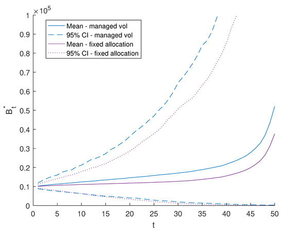
Figure 1.
The confidence interval of annuity payments. Managed-Volatility vs. Fixed Allocation (65%/35%)—Nominal.
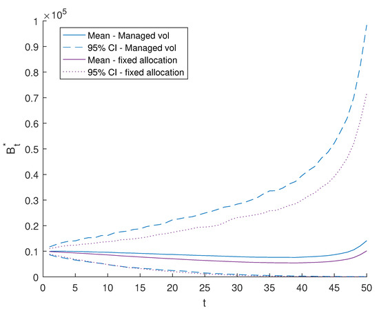
Figure 2.
The confidence interval of annuity payments. Managed-Volatility vs. Fixed Allocation (65%/35%)—Real.
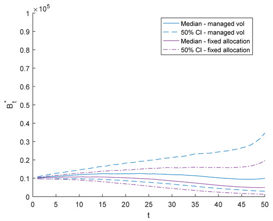
Figure 3.
The confidence interval of annuity payments. Managed-Volatility vs. Fixed Allocation (65%/35%)—Nominal.
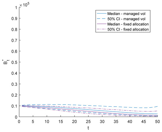
Figure 4.
The confidence interval of annuity payments. Managed-Volatility vs. Fixed Allocation (65%/35%)—Real.
The managed-volatility strategy outperforms the fixed allocation strategy having a higher mean payment as well as higher upside. There is little visible difference in terms of downside for annuity payments. In real terms, the mean annuity payments show a slow trend downwards, reaching a minimum amount of AUD 7590 after 39 years at age 89.
Table 3 shows the annuity payments at the older ages of 80 and 90. The managed-volatility strategy consistently generates a higher mean annuity payment, as well as higher annuity payment amounts at the and percentiles compared to the fixed balanced asset allocation strategy.
Table 3.
Base Case: Annuity Payments at Age 80 and 90—Nominal.
Table 4 shows the present value of annuity payments at the pricing interest rate for comparison. These amounts are not risk-adjusted, but quantify the higher amount of expected annuity payments from the managed-volatility strategy. In nominal terms, the mean of the PV of annuity payments of the managed-volatility strategy is 22.7% higher than the fixed asset allocation, while in real terms, the mean of the managed-volatility strategy is 18.3% higher than the fixed allocation. On the upside, for the 97.5% percentile, the target volatility strategy is 25.7% higher in nominal values and 20.8% in real values. On the downside, for the 2.5% percentile, the target volatility strategy is 9.6% higher in nominal values and 5.2% in real values.
Table 4.
Base Case: PV Annuity Payments—Nominal vs. Real.
Table 5 shows that on average it takes 15 years for a participant in the managed-volatility strategy to break even, while it takes 17 years for a participant in the fixed allocation strategy to break even. Neither strategy breaks even at the lower bound of the confidence interval, hence the ‘NA’ at the percentile, and it takes one more year for the fixed allocation strategy to break even on the higher end of the confidence interval.
Table 5.
Base Case: Break Even Year—Nominal.
Table 6 and Table 7 show the values for the CV and CDD of the two strategies over time. There is little difference between the managed-volatility strategy and the fixed allocation strategy. Early on the managed-volatility has slightly lower CV and CDD, whereas the fixed allocation strategy is lower than the managed-volatility strategy at the older ages. The higher managed-volatility CV reflects the impact of the higher target volatility at older ages.
Table 6.
Coefficient-of-Variation of Annuity Payments.
Table 7.
Coefficient-of-Downside Deviation of Annuity Payments.
4.3. Equity Asset Allocation
The asset allocation in practice will reflect the risk appetite of the pooled annuity fund. We first consider the strategies without volatility management. These strategies are most similar to the standard asset management practice for life annuities. The three strategies chosen to compare the investment returns at different levels of risks are:
- 100% 3-month fixed-income;
- 100% 10-year fixed-income;
- 80% fixed-income, 20% equity, without volatility management.
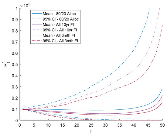
Figure 5.
Annuity Payment Comparison—Without Volatility Management.
Table 8.
Annuity Payment at Age 80 and 90 without volatility management—Nominal.
The asset portfolio consisting only of the 3-month fixed-income, which is the least risky, produces the lowest mean payments along with the narrowest confidence interval. On the other hand, the portfolio with 20% equity and 80% long term fixed-income, produces the highest mean return along with the widest confidence interval. As expected, as the allocation to equity increases, the mean annuity payment increases and the confidence interval widens.
We then consider different asset allocations including a more aggressive and a more defensive equity strategies under the managed-volatility framework. In particular, we consider and compare three sets of equity asset allocations:
- 4.
- 80% fixed-income, 20% equity;
- 5.
- 65% fixed-income, 35% equity;
- 6.
- 50% fixed-income, 50% equity.
Allocation 4 represents a conservative strategy for those with lower risk tolerance. Allocation 5 represents the balanced fund. Allocation 6 represents an aggressive strategy for those with a higher risk appetite. The mean annuity payments and the 95% confidence intervals for ages 80 and 90 are shown in Table 9.
Table 9.
Annuity Payments at Different Initial Allocations at Age 80 and 90.
We see that in all cases the managed-volatility strategy produces higher mean annuity payments at these older ages. The higher the equity exposure is the larger is the difference between the managed-volatility strategy and the fixed allocation strategy. The managed-volatility strategy has a higher downside as well as a higher upside.
The PV annuity payment amounts are shown in Table 10.
Table 10.
PV Annuity Payments at Different Initial Allocations.
The benefits of higher equity exposure are shown in the PV of annuity payments. Even though the values are not risk adjusted, the higher mean PVs for the managed-volatility strategy, along with the reduced downside, shows that the managed-volatility strategy adds value over and above the fixed allocation strategy.
The BEYs are shown in Table 11. Portfolios with a higher allocation in equity require on average a shorter time to break even with a slightly shorter time required for the managed-volatility strategy. However, it is worth highlighting the higher risk of the strategies with higher allocation in equity which have a chance of not breaking even as indicated by the ‘NAs’ at the percentile for the 80%/20% and the 65%/35% strategies.
Table 11.
Break Even Years at Different Initial Allocations.
4.4. Varying the Level of Target Volatility
The level of target volatility should reflect the risk appetite of the fund. The higher the target volatility, the higher the overall exposure to the equity market, and therefore the higher the overall investment risk. We consider two target volatility strategies:
- Constant target volatility;
- Target volatility that decreases over time.
The constant target volatility aims to ensure the equity investment strategy is not exposed to varying volatility and hence varying levels of equity market risk. In the later ages we observe an increase in the mean annuity payment in the pooled fund reflecting the smaller pool size and the benefit of larger mortality credits. This allows a strategy to decrease the target volatility over time while maintaining the mean level of annuity payment.
Table 12 and Table 13 show the annuity payments at age 80 and 90 as well as the PV of the annuity payments at the pricing interest rate for differing target volatilities. This includes a level of target volatility equal to the historical volatility. Even in this case, the managed-volatility strategy produces a higher mean annuity payment as well as higher downside and upside annuity payments. The PVs of the annuity payments are also higher for the managed-volatility strategy. In all cases in this section and in Section 4.5, we assume an initial asset allocation of 65% in long-term fixed-income asset and 35% in equity.
Table 12.
Annuity Payments at Different Fixed Target Volatilities at Age 80 and 90.
Table 13.
PV Annuity Payments at Different Fixed Target Volatilities.
For increased levels of target volatility, the mean annuity payments increase as do the downside and upside values.
Table 14 shows that the fixed allocation strategy takes longer until break even, although there are only small differences with the target volatility strategies.
Table 14.
Break Even Years at Different Fixed Target Volatilities.
Figure 6 shows the mean of as age increases to illustrate the average mortality gain. The mean mortality experience gain is most significant in the last 10 years at ages of 90 and above.
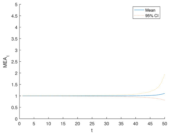
Figure 6.
Mortality experience adjustment, .
We consider two strategies to lower the target volatility after age 90. The first strategy linearly “trends down” from the initial target level to zero in the last 40 quarters. The second strategy “steps down” from the initial target level. For the last 40 to 20 quarters, the target volatility is reduced to 50% of the initial target level and for the last 20 quarters it is reduced to zero. These are based on the 1.25 historical volatility target.
The comparison of these strategies and the fixed target volatility strategy are given in Figure 7 and Figure 8. Both of these strategies produce lower mean annuity payments with little change in the downside and upside annuity payments. The decreasing target volatility lowers the expected payment outcomes in the last 10 years, or 40 quarters. The more drastic the decrease, the more significant the impact. The impact is asymmetric on the upside and downside. The lower bound of the 95% confidence interval suffers less impact than the higher bound.

Figure 7.
Fixed Volatility vs. “Trend Down” Volatility—Real.
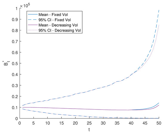
Figure 8.
Fixed Volatility vs. “Step Down” Volatility—Real.
The PV annuity payments comparison is shown in Table 15. There is limited difference from the fixed target-volatility strategy.
Table 15.
PV Annuity Payments at Different Target Volatilities.
Table 16 shows that the BEYs for the three strategies are the same. The decreasing target volatility strategies do not impact break even levels reflecting the limited differences arising from mitigating equity volatility risk at older ages.
Table 16.
Break Even Years at Different Target Volatilities.
Although the target volatility level can impact the annuity payments, for any given level of equity volatility the use of a managed volatility strategy will produce higher expected annuity payments and improve the downside of the annuity payments.
4.5. Pool Size with Equity Investments
Qiao and Sherris (2013) assumed a conservative investment strategy with stochastic interest rates. Larger pool sizes produced a more constant mean annuity payment at older ages.
Adding equity to a pooled annuity has the potential to undermine the benefits of pooling mortality risk from increased equity volatility. We consider the impact of pool size when using a managed-volatility strategy. Figure 9 shows the mean annuity payments, along with confidence intervals, for initial pool sizes of 10, 50 and 100. For the smaller pool sizes there is a decrease in the mean annuity payments at the older ages. This does not occur for the larger pool sizes. In fact pool sizes of 100 or larger are sufficient for the mean and confidence intervals for the annuity payments to be similar regardless of pool size.
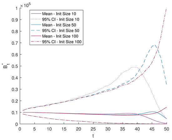
Figure 9.
Initial Pool Size Comparison: 10 vs. 50 vs. 100—Real.
Figure 10 shows that funds with initial sizes higher than 100 have similar and more constant mean annuity payments at the older ages. A larger fund with 10,000 initial participants has slightly narrower confidence intervals in the last five years compared to a fund with 100 initial participants, but the difference is relatively small. In fact, the size of the fund can be quite small to benefit from pooling idiosyncratic mortality risks when equity is added to the investments in the fund.
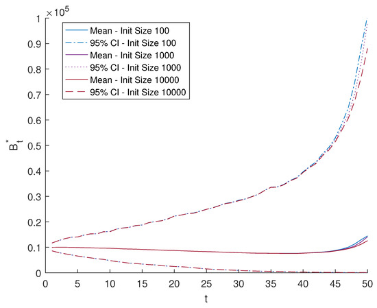
Figure 10.
Initial Pool Size Comparison: 100 vs. 1k vs. 10k—Real.
5. Discussion
Our analysis has considered, for the first time, the impact of equity investments on pooled annuity payments using a group self annuitization payment structure, that aims to produce relatively constant expected annuity payments, incorporating a simple target volatility investment strategy. Pooled annuity products are attracting increasing attention as a practical and cost effective method of annuitization compared with the traditional fixed life annuity.
Our results and analysis have clear and important implications for product design of pooled annuities, in particular, for defined contribution funds facing the challenge of providing annuity income in retirement in a cost-effective and fair manner, at the same time aiming to provide exposure to equity investments that increase expected payments consistent with risk preferences for their members.
In Australia, this is a major focus of retirement income policy (Australia Government the Treasury 2020). Our analysis informs this policy issue, not only for Australia but for all countries with defined contribution funds facing the challenge of providing an annuity that combines the benefits of mortality pooling with exposure to equity investments.
We show how it is practical to incorporate equity investments in a pooled annuity fund combining the benefits of exposure to equity returns post retirement with the benefits of pooling mortality. Although these benefits have been highlighted in the literature, there has been no detailed analysis of the impact on annuity payments using a range of risk measures compared with expected annuity payments at differing ages.
Consistent with other studies, such as Qiao and Sherris (2013) and Stamos (2008), we confirm the effectiveness of pooled annuities even for relatively small pool sizes.
Our focus has been on a single cohort in the pooled annuity. These results extend naturally to multiple cohorts based on Qiao and Sherris (2013) and Milevsky and Salisbury (2016). Results can also be extended to take into account inflation by designing annuity payment streams that increase through time (Qiao and Sherris 2013).
6. Conclusions
The growing demand for retirement income products and recent developments in target volatility risk management strategies for equity portfolios provides our motivation to consider investment strategy innovations for pooled annuity products. We are the first to assess a managed volatility equity strategy for pooled annuity products. We use models calibrated to Australian data to assess the impact of including equity investments, along with a managed volatility strategy, on pooled annuity payments and the present value of pooled annuity payments.
We add to the literature by showing that equity investments can improve the value of a pooled annuity product for those in the pool. We also show that the managed volatility strategy improves the value of pooled annuity products in terms of higher mean annuity payments, lower volatility and lower downside risk. We show that when equity investments are included in the portfolio a relatively small pool size, as low as 100 lives, is all that is required to reduce the impact of idiosyncratic mortality on the annuity payments in the fund especially at the older ages.
Author Contributions
Conceptualization, M.S.; data curation, S.L.; formal analysis, S.L.; investigation, S.L.; supervision, H.L.H., M.S. and A.M.V.; writing—original draft preparation, S.L.; writing—review and editing, H.L.H., M.S. and A.M.V.; funding acquisition, M.S. and A.M.V. All authors have read and agreed to the published version of the manuscript.
Funding
The authors acknowledge financial support from the Society of Actuaries Center of Actuarial Excellence Research Grant 2017–2020: Longevity Risk: Actuarial and Predictive Models, Retirement Product Innovation, and Risk Management Strategies as well as support from CEPAR Australian Research Council Centre of Excellence in Population Ageing Research project number CE170100005.
Data Availability Statement
We used publicly available data in this study. The mortality data for Australia are available on the Human Mortality Database (https://www.mortality.org/, accessed on 1 June 2018). The GDP, CPI and short term interest data for the economics scenario generator are available from the Reserve Bank of Australia (https://www.rba.gov.au/statistics/, accessed on accessed on 1 May 2018). Equity returns from the stock index ASX All Ordinaries are available from the Wall Street Journal (https://www.wsj.com/market-data/quotes/index/AU/XASX/XAO, accessed on accessed on 1 May 2018).
Conflicts of Interest
Michael Sherris is a Co-Founder and Director of the UNSW staff spinout Qforesight Pty Ltd., established to commercialise Target Volatility research carried out at UNSW and subsequently developed for commercial application.
Appendix A. Mortality Model, Estimated Parameters and Simulation
The calibrated parameters for the two-factor Blackburn Sherris model are given in Table A1.
Table A1.
Mortality Model Parameters.
Table A1.
Mortality Model Parameters.
| −0.1004 | −0.1347 | 1.4285 | 4.9659 |
In the mortality simulations, calendar year 2014 is used as , as it was the latest calendar year available in the HMD database. We consider a single age cohort with x set at age 50. The projected force of mortality and the survival function of systematic mortality from to are shown in Figure A1 and Figure A2. The results are based on 1000 simulated paths, which are consistent with the results in Section 4.2, Section 4.3, Section 4.4 and Section 4.5. Here the survival function is given by:

Figure A1.
Simulated Force of Mortality From 2014.
Figure A1.
Simulated Force of Mortality From 2014.


Figure A2.
Simulated Survival Function From 2014.
Figure A2.
Simulated Survival Function From 2014.

Appendix B. Economic Series Data, Estimation and Simulations
The economic series data used to calibrate the VAR model are shown in Figure A3, Figure A4, Figure A5 and Figure A6. The impact of financial crisis of 2007 to 2008 is evident in Figure A5. The short term interest rate in Figure A6 demonstrates a generally decreasing trend in this period.

Figure A3.
Real GDP (GDP).
Figure A3.
Real GDP (GDP).


Figure A4.
CPI (CPI).
Figure A4.
CPI (CPI).


Figure A5.
All Ordinaries Accumulated (XAOA).
Figure A5.
All Ordinaries Accumulated (XAOA).


Figure A6.
Short Term Yield (STY).
Figure A6.
Short Term Yield (STY).

In the VAR model, we the log scale of the series, as the growth of the series are more of interest than the absolute values. Figure A7 compares the log scale series. It is observed that , , and tend to trend up together, though cointegration is not shown to be significant.

Figure A7.
Log Scale Data.
Figure A7.
Log Scale Data.

Appendix B.1. Cointegration Test for VAR Model
Appendix B.1.1. Stationarity at Level
Before applying cointegration test, we first perm a stationarity test to the series at level. We performed the Augmented Dickey–Fuller (ADF) test on , , and at significance level of 0.05. The test result fails to reject null hypothesis of no unit root for all series. This implies that unit root exists, and that the series at level are not stationary. KPSS test gives the same inference.
Table A2.
ADF Unit Root Test at Level.
Table A2.
ADF Unit Root Test at Level.
| Aug D-F Test (at Level) | ||||
|---|---|---|---|---|
| P-Value | 0.9990 | 0.9990 | 0.9990 | 0.3199 |
| Null Hypothesis Result | not rejected | not rejected | not rejected | not rejected |
| Stationarity | no | no | no | no |
The four series are then tested for cointegration using Johansen test.
Appendix B.1.2. Johansen Test
With the ‘Trace’ test, the Johansen test assesses the null hypothesis that cointegration rank is less than or equal to r, against the alternative that is 4, which is the dimension of vector in this case. The test is carried out at significance level of 0.05 and lag 1. The test results are summarized in Table A3.
Table A3.
Johansen Test.
Table A3.
Johansen Test.
| r | h | stat | cValue | pValue | eigVal |
|---|---|---|---|---|---|
| 0 | 0 | 46.0198 | 47.8564 | 0.0737 | 0.2351 |
| 1 | 0 | 24.8498 | 29.7976 | 0.1672 | 0.1396 |
| 2 | 0 | 12.9739 | 15.4948 | 0.1163 | 0.1142 |
| 3 | 0 | 3.3944 | 3.8415 | 0.0654 | 0.0421 |
The test result shows that it fails to reject the null hypothesis at to . This means that no significant cointegration relationship is found in the vector at significance level of 0.05. While we acknowledge that the test result does not imply that there is no cointegration between the series, it supports the choice for a VAR model as the ESG, which is simpler than options such as VECM, and fits the purpose of this project.
Appendix B.2. Stationarity Test at First Difference for VAR Model
As cointegration is not significant in the vector, the model reduces to a VAR model at first difference. To start with, we take the first difference of the log scale series and test for stationarity, as shown in Figure A8 and Table A5. The descriptive statistics of the differenced series are summarized in Table A4.

Figure A8.
First difference of Log Scale Data.
Figure A8.
First difference of Log Scale Data.

Table A4.
Descriptive Statistics at First Difference.
Table A4.
Descriptive Statistics at First Difference.
| Statistic | ||||
|---|---|---|---|---|
| Mean | 0.0066 | 0.0223 | 0.0079 | −0.0005 |
| Std Dev | 0.0057 | 0.0693 | 0.0055 | 0.0053 |
| Skewness | 1.9863 | −0.8634 | 0.5771 | −1.0974 |
| Kurtosis | 12.6015 | 4.6751 | 5.2732 | 14.2357 |
| First Quantile | 0.0030 | −0.0108 | 0.0047 | −0.0021 |
| Median | 0.0063 | 0.0273 | 0.0077 | 0.0001 |
| Third Quantile | 0.0091 | 0.0663 | 0.0112 | 0.0021 |
| Min | −0.0045 | −0.2256 | −0.0068 | −0.0286 |
| Max | 0.0377 | 0.1952 | 0.0296 | 0.0218 |
The ADF test shows that the first difference series do not have unit roots, and are hence stationary, as shown in Table A5.
Table A5.
ADF Unit Root Test at First Difference.
Table A5.
ADF Unit Root Test at First Difference.
| Aug D-F Test (First Difference) | ||||
|---|---|---|---|---|
| p-value | 0.0010 | 0.0010 | 0.0010 | 0.0010 |
| Null Hypothesis result | rejected | rejected | rejected | rejected |
| stationarity | yes | yes | yes | yes |
Appendix B.3. Optimal Number of Legs for VAR Model
Four lags are tested for the VAR model. Akaike Information Criterion (AIC) of VAR(1) to VAR(4) are calculated and summarized in Table A6. AIC of lag 1 is the lowest of the four candidates. Therefore the VAR model is fitted at lag 1.
Table A6.
VAR AIC.
Table A6.
VAR AIC.
| VAR (1) | VAR (2) | VAR (3) | VAR (4) | |
|---|---|---|---|---|
| AIC | −2.1280 | −2.1154 | −2.0959 | −2.0854 |
Appendix B.4. Estimated Parameters for VAR Model
The parameters calibrated for the VAR model are:
and
Appendix B.5. Simulation Versus Actual Results
The VAR(1) model is used to generate 10,000 simulations from 30 September 1994 to 30 September 2015, to compare against the actual values from this period. The data from the four periods prior to 30 September 1994 are designated as ‘pre-sample’ to provide lagged data for VAR model estimation. The data from the six periods after 30 September 2015 are designated as ‘out-of-sample’ data for the purpose of backtesting.
The descriptive statistics of the comparison are summarized in Table A7.
Table A7.
Descriptive Statistics—Comparison.
Table A7.
Descriptive Statistics—Comparison.
| Simulation | Actual | |||||||
|---|---|---|---|---|---|---|---|---|
| Statistic | ||||||||
| Mean | 0.0067 | 0.0223 | 0.0080 | −0.0005 | 0.0066 | 0.0223 | 0.0079 | −0.0005 |
| Std Dev | 0.0001 | 0.0007 | 0.0001 | 0.0001 | 0.0057 | 0.0693 | 0.0055 | 0.0053 |
| Skewness | −0.2898 | −0.4418 | −0.3923 | −0.0616 | 1.9863 | −0.8634 | 0.5771 | −1.0974 |
| Kurtosis | 2.4385 | 3.5483 | 2.9874 | 4.0682 | 12.6015 | 4.6751 | 5.2732 | 14.2357 |
| First Quantile | 0.0066 | 0.0220 | 0.0080 | −0.0005 | 0.0030 | −0.0108 | 0.0047 | −0.0021 |
| Median | 0.0067 | 0.0224 | 0.0080 | −0.0005 | 0.0063 | 0.0273 | 0.0077 | 0.0001 |
| Third Quantile | 0.0067 | 0.0228 | 0.0080 | −0.0004 | 0.0091 | 0.0663 | 0.0112 | 0.0021 |
| Min | 0.0065 | 0.0203 | 0.0079 | −0.0006 | −0.0045 | −0.2256 | −0.0068 | −0.0286 |
| Max | 0.0068 | 0.0242 | 0.0081 | −0.0003 | 0.0377 | 0.1952 | 0.0296 | 0.0218 |
References
- Australia Government the Treasury. 2018. Retirement Income Disclosure Consultation Paper; Discussion Paper. Available online: https://treasury.gov.au/consultation/c2018-t347107 (accessed on 3 March 2022).
- Australia Government the Treasury. 2020. Retirement Income Review; Final Report. Available online: https://treasury.gov.au/publication/p2020-100554 (accessed on 3 March 2022).
- Blackburn, Craig, and Michael Sherris. 2013. Consistent dynamic affine mortality models for longevity risk applications. Insurance: Mathematics and Economics 53: 64–73. [Google Scholar] [CrossRef]
- Bollerslev, Tim. 1986. Generalized autoregressive conditional heteroskedasticity. Journal of Econometrics 31: 307–327. [Google Scholar] [CrossRef]
- Chen, An, Manuel Rach, and Thorsten Sehner. 2020. On the optimal combination of annuities and tontines. ASTIN Bulletin 50: 95–129. [Google Scholar] [CrossRef]
- Cox, John C., Jonathan E. Ingersoll, Jr., and Stephen A. Ross. 1985. A theory of the term structure of interest rates. Econometrica: Journal of the Econometric Society 53: 385–407. [Google Scholar] [CrossRef]
- Donnelly, Catherine. 2015. Actuarial fairness and solidarity in pooled annuity funds. Astin Bulletin 45: 49–74. [Google Scholar] [CrossRef]
- Donnelly, Catherine, Montserrat Guillén, and Jens Perch Nielsen. 2013. Exchanging uncertain mortality for a cost. Insurance: Mathematics and Economics 52: 65–76. [Google Scholar] [CrossRef]
- Donnelly, Catherine, Montserrat Guillén, and Jens Perch Nielsen. 2014. Bringing cost transparency to the life annuity market. Insurance: Mathematics and Economics 56: 14–27. [Google Scholar] [CrossRef]
- Duan, Jin-Chuan, and Jean-Guy Simonato. 1999. Estimating and testing exponential-affine term structure models by kalman filter. Review of Quantitative Finance and Accounting 13: 111–135. [Google Scholar] [CrossRef]
- Engle, Robert F. 1982. Autoregressive conditional heteroscedasticity with estimates of the variance of united kingdom inflation. Econometrica: Journal of the Econometric Society 50: 987–1007. [Google Scholar] [CrossRef]
- Engle, Robert F., and Victor K. Ng. 1993. Measuring and testing the impact of news on volatility. The Journal of Finance 48: 1749–78. [Google Scholar] [CrossRef]
- Hainaut, Donatien, and Pierre Devolder. 2006. Life annuitization: Why and how much? ASTIN Bulletin 36: 629–54. [Google Scholar] [CrossRef]
- Harris, Glenn R. 1997. Regime switching vector autoregressions: A bayesian markov chain monte carlo approach. Paper presented at 7th International AFIR Colloquium, Cairns, Australia, August 13–15, Volume 1, pp. 421–451. [Google Scholar]
- Harris, Glen R. 1999. Markov chain monte carlo estimation of regime switching vector autoregressions. Astin Bulletin 29: 47–79. [Google Scholar] [CrossRef]
- Hocquard, Alexandre, Sunny Ng, and Nicolas Papageorgiou. 2013. A constant-volatility framework for managing tail risk. The Journal of Portfolio Management 39: 28–40. [Google Scholar] [CrossRef]
- Ignatieva, Katja, Andrew Song, and Jonathan Ziveyi. 2016. Pricing and hedging of guaranteed minimum benefits under regime-switching and stochastic mortality. Insurance: Mathematics and Economics 70: 286–300. [Google Scholar]
- James, Estelle, and Xue Song. 2001. Annuities Markets Around the World: Money’s Worth and Risk Intermediation. CeRP Working Papers 16/01. Turin: Center for Research on Pensions and Welfare Policies. [Google Scholar]
- Milevsky, Moshe A., and Thomas S. Salisbury. 2015. Optimal retirement income tontines. Insurance: Mathematics and Economics 64: 91–105. [Google Scholar] [CrossRef]
- Milevsky, Moshe A., and Thomas S. Salisbury. 2016. Equitable retirement income tontines: Mixing cohorts without discriminating. ASTIN Bulletin 46: 571–604. [Google Scholar] [CrossRef]
- Morrison, Steven, and Laura Tadrowski. 2013. Guarantees and Target Volatility Funds. Moody’s Analytics, September 2. [Google Scholar]
- Nelson, Daniel B. 1991. Conditional heteroskedasticity in asset returns: A new approach. Econometrica: Journal of the Econometric Society 59: 347–70. [Google Scholar] [CrossRef]
- OMeara, Taleitha, Aakansha Sharma, and Aaron Bruhn. 2015. Australia’s piece of the puzzle–why don’t australians buy annuities? Australian Journal of Actuarial Practice 3: 47–57. [Google Scholar]
- Papageorgiou, Nicolas A., Jonathan J. Reeves, and Michael Sherris. 2017. Equity Investing with Targeted Constant Volatility Exposure. FIRN Research Paper No. 2614828. Sydney: UNSW Business School. [Google Scholar]
- Pedersen, Hal, Mary Pat Campbell, Stephan L. Christiansen, Samuel H. Cox, Daniel Finn, Ken Griffin, Nigel Hooker, Matthew Lightwood, Stephen M. Sonlin, and Chris Suchar. 2016. Economic Scenario Generators: A Practical Guide. Practical Guide. Society of Actuaries: Society of Actuaries. [Google Scholar]
- Peijnenburg, Kim, Theo Nijman, and Bas J. M. Werker. 2016. The annuity puzzle remains a puzzle. Journal of Economic Dynamics and Control 70: 18–35. [Google Scholar] [CrossRef][Green Version]
- Piggott, John, Emiliano A. Valdez, and Bettina Detzel. 2005. The simple analytics of a pooled annuity fund. Journal of Risk and Insurance 72: 497–520. [Google Scholar] [CrossRef]
- Qiao, Chao, and Michael Sherris. 2013. Managing systematic mortality risk with group self-pooling and annuitization schemes. Journal of Risk and Insurance 80: 949–74. [Google Scholar] [CrossRef]
- Sherris, Michael, and Boqi Zhang. 2009. Economic Scenario Generation with Regime Switching Models. Research paper No. 2009ACTL05. Sydney: UNSW Business School. [Google Scholar]
- Stamos, Michael Z. 2008. Optimal consumption and portfolio choice for pooled annuity funds. Insurance: Mathematics and Economics 43: 56–68. [Google Scholar] [CrossRef]
- Ungolo, Francesco, Michael Sherris, and Yuxin Zhou. 2021. Multi-Factor, Age-Cohort, Affine Mortality Models: A Multi-Country Comparison. Working Paper, CEPAR. Kensington: UNSW. [Google Scholar]
- Valdez, Emiliano A., John Piggott, and Liang Wang. 2006. Demand and adverse selection in a pooled annuity fund. Insurance: Mathematics and Economics 39: 251–66. [Google Scholar] [CrossRef]


Publisher’s Note: MDPI stays neutral with regard to jurisdictional claims in published maps and institutional affiliations. |
© 2022 by the authors. Licensee MDPI, Basel, Switzerland. This article is an open access article distributed under the terms and conditions of the Creative Commons Attribution (CC BY) license (https://creativecommons.org/licenses/by/4.0/).