Article

Equivalent Risk Indicators: VaR, TCE, and Beyond

by
Silvia Faroni
1,2,
Olivier Le Courtois
1,* and
Krzysztof Ostaszewski
3
1
EMLyon Business School, 23, Avenue Guy de Collongue, CEDEX, 69134 Ecully, France
2
COACTIS (EA4161), Université de Lyon/Lyon 2, ISH, 14-16 Avenue Berthelot, 69007 Lyon, France
3
College of Arts and Science, Illinois State University (ISU), Normal, IL 61790-4520, USA
*
Author to whom correspondence should be addressed.
Risks 2022, 10(8), 142; https://doi.org/10.3390/risks10080142
Submission received: 31 May 2022 / Revised: 29 June 2022 / Accepted: 18 July 2022 / Published: 22 July 2022
(This article belongs to the Special Issue Actuarial Mathematics and Risk Management)

Abstract

:
While a lot of research concentrates on the respective merits of VaR and TCE, which are the two most classic risk indicators used by financial institutions, little has been written on the equivalence between such indicators. Further, TCE, despite its merits, may not be the most accurate indicator to take into account the nature of probability distribution tails. In this paper, we introduce a new risk indicator that extends TCE to take into account higher-order risks. We compare the quantiles of this indicator to the quantiles of VaR in a simple Pareto framework, and then in a generalized Pareto framework. We also examine equivalence results between the quantiles of high-order TCEs.

1. Introduction

In the second half of the twentieth century, developed market economies had undergone an inflationary period after World War II, followed by a disinflationary period that started in the early 1980s accompanied by less regulation and greater reliance on market forces. These developments resulted in improved economic performance, but also increased volatility and market pressure on financial institutions following traditional fixed capital standards. In order to address these developments, regulators have moved towards risk-based capital requirements for financial institutions, while also allowing gradual relaxation of certain rules of governance of financial institutions and replacing them with a principle-based approach.
The risk measures imposed by regulators on insurance companies share a common feature: they are all related to the behavior of tails of the probability distribution of a firm’s financial results. The reason is that the regulatory purpose of capital requirements is to make capital available for absorbing losses occurring in extreme events, i.e., events of large financial losses, which could bring about insolvency. Risk-based capital requirements are a natural outgrowth of traditional prudential regulation aiming at preserving the solvency of private financial institutions.
Hence, safety capital should be computed by looking at the extreme risks that can impact financial institutions in general and insurance enterprises in particular. However, regulators differ in their specification of the tail indicator that they recommend. Some regulators impose the use of quantiles of the distribution (value at risk, or VaR), while other regulators impose the use of partial moments (tail conditional expectation or TCE, or an equivalent measure of expected shortfall). Furthermore, regulators also differ in their choice of time horizon. Finally, they also differ in their choice of confidence level (i.e., probability value for the quantile, or for the conditional expectation).
Comité Européen des Assurances and Mercer Oliver Wyman Limited (2005) and CEA (2007) provide a comparison of different regulatory regimes for capital requirements. The most consequential regulation of risk-based capital is the European Union’s Solvency II. Solvency II imposes risk-based capital requirements computed using the VaR as a risk measure over a one-year period and with a confidence level of 99.5%. When Solvency II was being designed, it was to some degree modeled on the Basel II banking regulation, also using VaR as a risk measure for capital requirement purposes, for market risk. The credit crisis of 2008 in many ways exposed the weaknesses of VaR, and a new system of capital regulation for banking, Basel III (see Basel Committee on Banking Supervision’s documents from 2019 and 2022), has been developed and implemented since (see also Gatzert and Wesker (2011) for a comparison of Solvency II and Basel regulations).
Solvency II is not only the main regulatory law for prudential regulation of insurance enterprises in the European Union, but it has become a model for risk-based capital requirements worldwide. The United States is one major exception to this trend, as the U.S. model regulation of insurance firms’ capital preceded Solvency II, and it is designed around a formula provided by the regulatory body, the National Association of Insurance Commissioners (NAIC) (see also National Association of Insurance Commissioners (2007) on ORSA perspectives).
The Canadian regulation of insurance capital differs from that of the European Union, and it is based on risk assessment of the firm in the context of certain extreme events. Canada’s Office of Supervision of Financial Institutions (OSFI) risk assessment process begins with an evaluation of the inherent risk within each significant activity of an insurer and the quality of risk management applied to mitigate these risks (see Canada Office of Supervision of Financial Institutions 2022). After considering this information, OSFI determines the level of net risk and direction (i.e., whether it is decreasing, stable, or increasing) of the rating for each significant activity. The net risks of the significant activities are combined, by considering their relative importance, to arrive at the overall net risk (ONR) of the insurer. Furthermore, OSFI provides capital requirement guidelines, which must be then included in insurers’ own risk and solvency assessment.
In the cases of both the United States and Canada, we see a significant regulatory involvement in the supervision of risk-based capital. All regulators are, of course, involved in this process, but the approach of the European Union and, notably, Switzerland, is more principle-based than rule-driven. The Swiss regulation of risk-based capital for insurers includes a capital standard, and stress-testing of certain extreme scenarios. The capital standard is based on the expected shortfall, or, equivalently, tail conditional expectation (TCE).
In this work, we focus on two regulations: Solvency II and the Swiss Solvency Test (SST). The Swiss Solvency Test, implemented in 2004, preceded Solvency II, but in 2015 the European Union recognized the SST as the first regime to be fully equivalent to Solvency II. Solvency II imposes a capital requirement computed using value at risk (VaR) as a risk measure over a 1-year period and with a confidence level of 99.5 % , whereas SST uses TCE with a confidence level of 99 % over a 1-year period.
VaR and TCE are the most classic examples of risk measures (see for instance Linsmeier and Pearson 2000; Klugman et al. 2012; Acerbi et al. 2001). A risk measure is a mapping from the random variable representing risk exposure to the set of real numbers. It can be interpreted as the amount of capital required to protect against adverse outcomes of a given risk. The paper by Artzner et al. (1999) introduced the concept of coherence of risk measures and has been very influential in the further development of risk measurement. A coherent risk measure is defined by the following four properties: subadditivity, monotonicity, positive homogeneity, and translation invariance. The properties of risk measures in the context of insurance are discussed by Wang and Zitikis (2021). Acerbi and Tasche (2002) noted that TCE is a coherent risk measure, while VaR is not (see also Society of Actuaries (2000) on TCE).
Rostek (2010) provides an interesting alternative to evaluations of risk, a model of preferences, in which, given beliefs about uncertain outcomes, an individual evaluates an action by a quantile of the induced distribution. Fadina et al. (2021) designed a unified axiomatic framework for risk evaluation principles, which quantifies jointly a loss random variable and a set of plausible probabilities. They called such an evaluation principle a generalized risk measure.
Fuchs et al. (2017) show that a notion of a quantile risk measure is a natural generalization of that of a spectral risk measure and provides another view of the distortion risk measures generated by a distribution function on the unit interval. In this general setting, they prove several results on quantile or spectral risk measures and their domain with special consideration of the expected shortfall. They also present a particularly short proof of the subadditivity of the expected shortfall risk measure. Denuit et al. (2006) provide a comprehensive review or modeling risk in incomplete markets, with emphasis on insurance risks, expanding on and combining in a comprehensive review the existing literature on quantitative risk management.
Li and Wang (2022) noted that the Basel Committee on Banking Supervision proposed the shift from the 99 % value at risk (VaR) to the 97.5 % expected shortfall (ES) for internal models in market risk assessment (see Basel Committee on Banking Supervision 2019, 2022). Inspired by that development, Li and Wang introduced a new distributional index, the probability equivalence level of VaR and ES (PELVE), which identifies the balancing point for the equivalence between VaR and ES. PELVE has desirable theoretical properties, and it distinguishes empirically heavy-tailed distributions from light-tailed ones.
Barczy et al. (2022) generalized and further developed the PELVE measure and applied this indicator to a high-order TCE, which is distinct from the extended TCE introduced in the present paper. Fiori and Rosazza Gianin (2021) construct another generalization by constructing an indicator that relates monotone risk measures.
Our paper was developed independently from this stream of papers and develops related comparisons of VaR and TCE quantiles, but without introducing an intermediate indicator such as PELVE. A key contribution of our paper is the introduction of a new risk indicator that extends TCE to take into account higher-order risks. We also provide comparisons of this new indicator with more classic risk indicators.
More deeply, the goal of our paper is to understand how regulators choose such or such risk indicators for solvency computations. Thus, our goal is to understand the implicit utility function of insurance regulators and to understand how equivalent risk valuation systems can be put in place, but we do so without introducing any type of utility function. It is, of course, entirely possible that the regulations put in place are not fully a result of a certain intent, but rather of a political process so that what we determine may not be the output of an actual utility function of a specific regulator. However, making the implicit functioning of actual regulations explicit should be a valuable contribution in assuring that regulations function in an effective and efficient manner.
The paper makes use of two probabilistic assumptions, where we assume that claims can be either Pareto or generalized Pareto (GPD) distributed. We make these assumptions for two main reasons: they allow us to very conveniently derive readable results and they are consistent with what is observed for claims with heavily distributed tails. The reader interested in exploring situations where claims could be associated with semi-heavy tails can be referred for instance to Le Courtois (2018) or Le Courtois and Walter (2014).
The paper is organized as follows. In Section 2, we provide a general overview of the two main risk measures, VaR and TCE, and briefly discuss equivalence results that relate to the confidence levels of VaR and TCE. In Section 3, we introduce a new and generalized tail indicator, and we discuss the relation between the quantiles of this indicator and the quantiles of VaR, in a simple Pareto framework, and then in a generalized Pareto framework. Section 4 examines equivalence results between the quantiles of generalized indicators.

2. VaR and TCE

In this section, we recall key preparatory elements on VaR and TCE. We first recall classic definitions. Then, we examine the link between VaR and TCE. We conclude with an illustration of this link. These elements will be useful in the next section, where the core contribution of the paper is developed.

2.1. Definitions

The most used risk measure is value at risk (VaR), which is the expected worst loss over a given horizon at a given confidence level. Linsmeier and Pearson (2000) define VaR as the loss that is expected to be exceeded with a probability of only ( 1 α ) percent during the next holding period T. The role of regulators is to choose the value of the confidence level α and of the horizon T.
From a mathematical viewpoint, suppose that F X T ( x ) represents the distribution function of outcomes over a fixed period of time T of a portfolio of risks. An adverse outcome is a loss and, in this case, positive values of the random variable X T are losses. The VaR of the random variable is the α percentile of the distribution of X T , denoted by
VaR α ( X T ) = F X T 1 ( α ) .
According to the report of the National Association of Insurance Commissioners (2007), tail conditional expectation (TCE)—or conditional tail expectation (CTE)—measures the amount of risk within the tail of a distribution of outcomes, expressed as the probability-weighted average of the outcomes beyond a chosen point in the distribution.
In the report produced by the CEA (2007), TCE measures the average losses over the defined threshold (typically set as the VaR at a given confidence level α ). In other words, TCE is a conditional mean value, given that the loss exceeds the 1 α percentile. It is also often called tail value at risk (TVaR) or expected shortfall (ES). A broader analysis of TCE and its properties can be found in Society of Actuaries (2000). From a mathematical viewpoint, TCE is defined as follows:
TCE α ( X T ) = E X T | X T VaR α ( X T ) .
Furthermore, if the random variable is continuous, we can write:
TCE α ( X T ) = 1 1 α α 1 VaR u ( X T ) d u .

2.2. Relation between VaR and TCE Quantiles

If we compute VaR and TCE using the same quantile, TCE will be always higher than VaR, by construction. However, the quantiles for VaR and TCE are usually chosen to be different by regulators. We study which relation should exist between these two quantiles. Specifically, we examine how it is possible to find c and q such that VaR q = TCE c , where q > c . We conduct our analysis when risks follow a generalized Pareto distribution.
Let X T be a random variable that follows a generalized Pareto distribution with three parameters: location μ , scale σ , and shape ξ . The cumulative distribution function of X T admits the Jenkinson–von Mises representation, which can be expressed as follows:
F ( X T ) = 1 1 + ξ ( x μ ) σ 1 ξ ,
for ξ 0 .
In this situation, we can show that the VaR can be computed as follows:
VaR q ( X T ) = μ + 1 q ξ 1 · σ ξ ,
while the tail conditional expectation admits the following expression:
TCE c ( X T ) = μ + σ ξ 1 c ξ 1 ξ 1 .
To solve VaR q ( X T ) = TCE c ( X T ) , we first rewrite TCE c ( X T ) as a function of VaR c ( X T ) :
TCE c ( X T ) = 1 1 ξ · VaR c ( X T ) + σ ξ μ 1 ξ .
Thus, TCE c ( X T ) = VaR q ( X T ) is equivalent to
1 1 ξ · VaR c ( X T ) + σ ξ μ 1 ξ VaR q ( X T ) = 0 .
Using the above equality, we can relate the quantities c and q as follows.
Theorem 1.
In the generalized Pareto framework, the quantile of TCE and the quantile of VaR obey the following relationship when the two risk indicators are equal:
c = 1 1 ξ 1 ξ · 1 q
where 0 < ξ < 1 .
Proof. 
See Appendix A. □
Note that Equation (4) depends on ξ , but not on μ or σ . Also note that if ξ = 1 α , the result obtained using the generalized Pareto distribution boils down to an identical result in the subcase of Pareto Type I distributions.

2.3. Illustration

Next, we illustrate Theorem 1 in Figure 1, where we plot the TCE quantile as a function of its equivalent VaR quantile. We plot this relation for different values of the market risk parameter ξ , where we let ξ take values between 0.01 and 0.99 . We recall that a higher value of ξ is equivalent to an increased presence of extreme risks in the phenomenon under study.
We can see that when there is more risk on the market, that is, when ξ 1 , the VaR quantile has to be a number close to 1, whereas the TCE quantile can take a broad range of values between 0.9 and 1.
This feature implies that in the presence of a lot of extreme risks, there is a large variability in the choice of the TCE quantile, making it a difficult value to choose by regulators. Conversely, in the presence of a lot of extreme risks, the VaR quantile is easy to set, where the regulator only needs to choose a sufficiently high value, as is observed in the case of the Solvency II regulation.
However, this feature is not observed when ξ is small, where a lot of admissible values can be taken by both the VaR and TCE quantiles, and where these two quantiles vary linearly.
Figure 1 also illustrates that a lot of the solutions to Theorem 1 are consistent with the Solvency II and the Swiss insurance regulations. However, the figure also illustrates that the two regulations are inconsistent. Indeed, it is practically impossible to find a pair of reasonable values of the VaR and TCE quantiles that is consistent with both regulations.

3. A New High-Order TCE Indicator

In this section, we introduce a new generalized TCE indicator, which is a conditional higher-order moment of the probability distribution under study. We compute this indicator when losses follow a Type I Pareto distribution and we derive equivalence relations with value at risk. We also conduct a similar study when losses follow a generalized Pareto distribution.

3.1. Definition

By analogy with higher-order moments, which are key characteristics of probability distributions, we construct a higher-order measure of risk, which is a TCE at order m. We denote this indicator by TCE ( m ) and we define it as follows:
TCE c ( m ) ( X T ) = E X T m | X T VaR c ( X T ) .
As an illustration, TCE c ( 2 ) is a conditional non-central second-order moment, where the condition is that losses exceed the 1 c percentile. Further, TCE c ( 1 ) is the standard tail conditional expectation indicator.
Because
E X T m | X T VaR c ( X T ) = E X T m 1 X T VaR c ( X T ) P r X T VaR c ( X T ) ,
we can rewrite the extended TCE indicator as follows:
TCE c ( m ) ( X T ) = 1 1 c E X T m 1 X T VaR c ( X T ) ,
so that
TCE c ( m ) ( X T ) = 1 1 c VaR c ( X T ) + x m d F ( x ) ,
where c = F VaR c ( X T ) .
Let us change variables as follows: F ( x ) = s , x = F 1 ( s ) = VaR s ( X T ) , and d s = d F ( x ) . We readily obtain a third equivalent representation of the extended TCE indicator:
TCE c ( m ) ( X T ) = 1 1 c c 1 VaR s ( X T ) m d s .
Note that another extended TCE indicator Ξ ( m ) can be found in the risk management literature (see for instance Barczy et al. (2022)). This indicator is defined by:
Ξ ( m ) = m 1 c c 1 s c 1 c m 1 VaR s ( X T ) d s = m 1 c c 1 s c 1 c m 1 F 1 ( s ) d s .
If we again change variables as follows: F ( x ) = s , x = F 1 ( s ) = VaR s ( X T ) , and d s = d F ( x ) , we obtain:
Ξ ( m ) = m 1 c VaR c ( X T ) + F ( x ) c 1 c m 1 x d F ( x ) .
All of these expressions are distinct from Equations (5)–(7) and confirm that Ξ ( m ) cannot be interpreted as a conditional higher-order moment, contrary to the indicator examined in this paper.

3.2. Pareto Distributed Losses

Let us now assume that losses follow a Type I Pareto distribution, whose probability density function is represented by:
f X T ( x ) = α θ α x α + 1 ,
where α is the shape parameter and θ the scale parameter.
We apply the definition in Equation (6) to compute TCE ( m ) when losses follow a Type I Pareto distribution. We write:
TCE c ( m ) ( X T ) = 1 1 c VaR c ( X T ) + x m α θ α x α + 1 d x .
This expression can be developed in closed form as a function of value at risk, as shown in the next theorem.
Theorem 2.
When losses are Pareto distributed, the extended TCE indicator admits the following expression.
TCE c ( m ) ( X T ) = α α m VaR c ( X T ) m
when α > m .
Proof. 
See Appendix A. □
From this theorem, we deduce that VaR q ( X T ) = TCE c ( X T ) is equivalent to
α α m · VaR c ( X T ) m VaR q ( X T ) = 0 .
This equation allows us to find the relation between the extended TCE and the VaR quantiles. Indeed, we obtain:
Theorem 3.
In the Pareto framework, the extended TCE quantile (c) and the VaR quantile (q) obey the following relationship when the two risk indicators are equal:
c = 1 α m θ 1 m α α m 1 q 1 m .
Proof. 
See Appendix A. □
For consistency with the generalized Pareto approach, we replace the shape parameter α of the classic Pareto distribution with ξ = 1 α , which can also be interpreted as a shape parameter.
Thus, Equation (11) can be rewritten as follows:
c = 1 1 m ξ θ 1 m 1 m ξ 1 q 1 m ,
where 0 < ξ < 1 m .
It appears that Equation (12) generalizes the result of Theorem 1. Indeed, Equation (12) reduces to Equation (4) when m = 1 .
Figure 2 shows the extended TCE quantile as a function of the VaR quantile, for different values of the shape parameter ξ . In the left panel of Figure 2, the scale parameter is equal to θ = 1 , while the scale parameter is equal to θ = 5 in the right panel of this figure. Both panels are plotted assuming that m = 2 .
As in the case of Figure 1, we see that a higher value of the shape parameter leads to more intricate situations, where the VaR quantile takes a value close to one, while the extended TCE quantile can take a broad range of values. However, Figure 2 also shows that a higher value of the scale parameter leads to even more intricate situations. Thus, when value at risk is not able to distinguish between extreme risk situations, a more sophisticated indicator such as the extended TCE indicator is able to produce such a distinction.
Figure 3 is constructed in a similar way as Figure 2, but now both panels are plotted assuming that m = 3 . By comparing Figure 2 and Figure 3, we see that the curves are pushed to the right for higher values of m, all other parameters being equal. Thus, varying the value of m allows us to construct risk indicators that are more or less sensitive to the presence of extreme risks.

3.3. GPD Losses

Let us now generalize the previous study to the case where the loss random variable X follows a generalized Pareto distribution. In accordance with the cdf shown in Equation (1), we rely on the following probability density function:
f X T ( x ) = 1 σ 1 + ξ x μ σ 1 ξ 1 ,
which generalizes Equation (8) by introducing a location parameter μ . The scale parameter is now denoted by σ and the shape parameter is now ξ 0 . For information on the estimation of tail parameters, see for instance Hill (1975) or Hosking and Wallis (1987).
We obtain a quasi-closed-form formula for the extended TCE indicator in this setting. Indeed, we have:
Theorem 4.
In the GPD case, the extended TCE indicator can be computed as follows:
TCE c ( m ) ( X T ) = 1 1 c · VaR c ( X T ) + x m 1 σ 1 + ξ x μ σ 1 ξ 1 d x = 1 1 c 1 m 1 ξ + 1 1 ξ Γ m + 1 ξ Γ m + 1 Γ 1 + 1 ξ μ ξ σ σ 1 ξ μ ξ σ ξ m 1 c VaR c ( X T ) m + 1 ( m + 1 ) · σ μ ξ 2 F 1 1 , m 1 ξ + 1 ; m + 2 ; VaR c ( X T ) ξ μ ξ σ ,
where 2 F 1 ( · , · ; · ; · ) is the hypergeometric function, Γ ( · ) is the gamma function, 0 < ξ < 1 m , and VaR c ( X T ) = μ + σ ξ 1 c ξ 1 .
Proof. 
See Appendix A. □
To solve TCE c ( m ) ( X T ) = VaR q ( X T ) , we can equivalently solve:
1 1 c 1 m 1 ξ + 1 1 ξ Γ m + 1 ξ Γ m + 1 Γ 1 + 1 ξ μ ξ σ σ 1 ξ μ ξ σ ξ m ( 1 c ) VaR c ( X T ) m + 1 ( m + 1 ) σ μ ξ 2 F 1 1 , m 1 ξ + 1 ; m + 2 ; VaR c ( X T ) ξ μ ξ σ = VaR q ( X T ) .
To numerically solve Equation (15), the following three conditions must be met:
  • 0 < ξ < 1 m , to ensure the convergence of the integral in Equation (14) and to avoid the appearance of complex numbers in Equation (15).
  • μ ξ σ 0 , to avoid the appearance of complex numbers in Equation (15).
  • VaR c ξ μ ξ σ < 1 , which is a necessary property of the fourth parameter of the hypergeometric function.
Although Equation (15) does not admit closed-form solutions, we numerically solve it to show the relation between the TCE ( m ) quantile and the VaR quantile, as a function of the order m and of the three generalized Pareto distribution parameters ξ , μ , and σ .
We start by plotting in Figure 4 the relation between the TCE ( m ) and the VaR quantiles when m = 2 and σ = 0.1 . The left panel of the figure presents the situation where μ = 0.05 , while the right panel presents the situation where μ = 0.05 .
From Figure 4, we see that the location parameter μ has a sharp impact on quantile dependences. When μ is high, the relation between indicator quantiles becomes nearly linear, which is an ideal situation from a risk management viewpoint.
Next, we plot in Figure 5 the relation between the TCE ( m ) and the VaR quantiles when m = 2 and μ = 0 . The left panel of the figure presents the situation where σ = 0.1 , while the right panel presents the situation where σ = 0.4 . From the comparison of the two panels of the figure, we see that the ideal situation where the relation between the indicator quantiles is quasi-linear occurs for small values of the scale parameter σ .
Finally, we plot in Figure 6 the relation between the TCE ( m ) and the VaR quantiles when m = 3 , μ = 0 . We set σ = 0.1 in the left panel and σ = 0.4 in the right panel. Thus, Figure 6 presents the same comparison as Figure 5, but for a larger value of the order parameter m.
From the comparison of Figure 5 and Figure 6, we see that higher values of the order parameter m lead to more intricate situations from a management viewpoint. Thus, the presence of extreme risks in the system being considered, and their taking into account via higher-order conditional moments, makes risk management more complicated in the sense that choosing an indicator quantile becomes a more critical and sensitive decision.

4. Equivalence between High-Order Indicators

In this section, we study the relation between the quantiles q ( m ) and q ( n ) of distinct extended tail conditional expectation indicators, where each indicator is associated with a different order m or n. Namely, we examine the situation where:
TCE q ( m ) ( m ) ( X T ) = TCE q ( n ) ( n ) ( X T ) .
We also study the sub-case where TCE is compared with a high-order TCE, that is, we study the quantiles q and q ( m ) that satisfy:
TCE q ( X T ) = TCE q ( m ) ( m ) ( X T ) .

4.1. Pareto Distributed Losses

If we model losses as random variables that follow a classic type I Pareto distribution, we can use Equation (9) to compute TCE q ( m ) ( m ) ( X T ) where α > m . Thus, we can compare two higher-order TCEs as follows:
α α m VaR q ( m ) ( X T ) m = α α n VaR q ( n ) ( X T ) n ,
where
VaR q ( m ) ( X T ) = θ 1 q ( m ) 1 α .
We obtain:
α α m θ m 1 q ( m ) m α = α α n θ n 1 q ( n ) n α ,
which leads us to:
q ( n ) = 1 α n α m θ m n α n 1 q ( m ) m n
where α > m , α > n , and θ > 0 .
If we denote ξ = 1 α , we can rewrite Equation (18) as in the following proposition.
Proposition 1.
When losses follow a classic Pareto distribution, the quantiles of high-order TCEs that solve Equation (16) can be related as follows:
q ( n ) = 1 1 ξ m 1 ξ n 1 ξ n θ n m ξ n 1 q ( m ) m n ,
where 0 < ξ < 1 m , 0 < ξ < 1 n , and θ > 0 .
We now illustrate this proposition.
Figure 7 plots the relation between the quantiles q ( m ) and q ( n ) when m = 5 and n = 2 . The left panel of the figure shows the situation where θ = 1 , while the right panel of the figure shows the situation where θ = 2 .
The left panel of Figure 7 can be interpreted as follows. The relation between the high-order quantiles is countermonotonic contrary to the relation between the TCE quantile and the VaR quantile, for instance. This means that a high value of q ( m ) corresponds to a small value of q ( n ) , and conversely.
This feature is a consequence of the fact that high-order TCEs concentrate on different parts of probability tails. Thus, the figure shows us that a manager that reduces high-order extreme risks at a given order, say m, is not simultaneously reducing high-order extreme risks at another order, say n. The right panel of the figure tells us that this aspect is even more pronounced for higher values of θ .
We now come to the specific case where n = 1 , that is to the study of the relation between TCE and a higher-order TCE:
α α 1 VaR q ( X T ) 1 = α α m VaR q ( m ) ( X T ) m .
Equation (18) becomes
q = 1 α m α 1 θ m 1 α 1 q ( m ) m ,
when α > m and θ > 0 . Similarly, Equation (19) becomes
q = 1 1 ξ m 1 ξ 1 θ m 1 1 ξ 1 q ( m ) m
when 0 < ξ < 1 m and θ > 0 .
We show in Figure 8 the relation between the TCE quantile and the high-order TCE quantile when m = 2 . The left panel of the figure shows the situation where θ = 1 , while the right panel of the figure shows the situation where θ = 2 .
Figure 8 confirms the results of Figure 7. Reducing risks using TCE does not necessarily reduce risks as measured by a high-order TCE, and conversely. Again, this effect is more pronounced for higher values of θ .

4.2. GPD Losses

Let us now come to the more general situation where losses are modeled using a generalized Pareto distribution. Our goal is to solve Equation (16) when the extended TCE indicator TCE q ( m ) ( m ) is given by Equation (14). Thus, to derive the relation between q ( m ) and q ( n ) , we numerically solve:
1 1 q ( m ) 1 m 1 ξ + 1 1 ξ Γ m + 1 ξ Γ m + 1 Γ 1 + 1 ξ μ ξ σ σ 1 ξ μ ξ σ ξ m 1 q ( m ) VaR q ( m ) ( X T ) m + 1 ( m + 1 ) · σ μ ξ 2 F 1 1 , m 1 ξ + 1 ; m + 2 ; VaR q ( m ) ( X T ) ξ μ ξ σ = 1 1 q ( n ) 1 n 1 ξ + 1 1 ξ Γ n + 1 ξ Γ n + 1 Γ 1 + 1 ξ μ ξ σ σ 1 ξ μ ξ σ ξ n 1 q ( n ) VaR q ( n ) ( X T ) n + 1 ( n + 1 ) · σ μ ξ 2 F 1 1 , n 1 ξ + 1 ; n + 2 ; VaR q ( n ) ( X T ) ξ μ ξ σ
Figure 9 plots the relation between the quantiles q ( m ) and q ( n ) when m = 5 , n = 2 , and σ = 0.1 . The left panel of the figure shows the situation where μ = 0.05 , while the right panel of the figure shows the situation where μ = 0.05 .
From Figure 9, we deduce that the link between the high-order TCE quantiles is linear when σ = 0.1 , so this parameter of the GPD distribution is not problematic. By comparing the two panels of the figure, we see that the parameter μ has little effect on the curves linking the high-order TCE quantiles.
Figure 10 plots the relation between the quantiles q ( m ) and q ( n ) when m = 5 , n = 2 , and μ = 0 . The left panel of the figure shows the situation where σ = 0.1 , while the right panel of the figure shows the situation where σ = 0.4 .
Figure 10 shows us that high values of σ can yield problematic links between the high-order TCE quantiles, hinting at probability tails that are quantified differently by distinct high-order TCE indicators.
We now come to the specific case where n = 1 , that is, to the study of the relation between TCE and a higher-order TCE. In that case also, the solutions are numerically obtained by solving Equation (20).
Figure 11 plots the relation between the quantiles q ( m ) and q when m = 2 and σ = 0.1 . The left panel of the figure shows the situation where μ = 0.05 , while the right panel of the figure shows the situation where μ = 0.05 .
Figure 11 tells us that the link between the second order TCE quantile and the TCE quantile is close to linear when σ = 0.1 , so that, again, this parameter of the GPD distribution is not problematic when it is not set to a high value.
By comparing the two panels of Figure 11, we see, as in Figure 9, that large variations of the parameter μ have a quite limited impact on the position of the curves relating a high-order TCE quantile to the TCE quantile.
Figure 12 plots the relation between the quantiles q ( m ) and q when m = 2 and μ = 0 . The left panel of the figure shows the situation where σ = 0.1 , while the right panel of the figure shows the situation where σ = 0.4 .
Figure 12 confirms the conclusion of Figure 10. Specifically, high values of σ can yield problematic links between a high-order TCE quantile and the TCE quantile.

5. Conclusions

We end this paper with a brief illustration based on actual data. We use a fire insurance claim data set, labeled “beaonre” within the R package CASdatasets. This dataset includes 1823 observations of fire insurance claims from the year 1997. We transform this dataset of claim costs into a dataset of reimbursements, from which we can compute VaR, TCE, and TCE ( m ) . To compare VaR or TCE with a high-order TCE indicator, we need to adjust the latter quantity in terms of scale. For instance, we may want to solve VaR q X T = TCE c ( m ) X T 1 m . While exact solutions to this equation do not exist, we can still deduce a relation between VaR and TCE ( m ) .
We show in Figure 13 the link between VaR and the high-order TCE indicator (computed with m = 2 ) in the case of fire data. This figure is consistent with the theoretical results shown, for instance, in Figure 6. Thus, Figure 13 confirms, in passing, the relevance of the GPD assumption. Further illustration with actual data is out of the scope of the present paper but could be a matter of an interesting extension.
To conclude, we introduce in this paper a new risk indicator that is a high-order TCE risk measure. We compare the quantiles of this indicator to the quantiles of VaR in a simple Pareto framework, and then in a generalized Pareto framework. We also examine equivalence results between the quantiles of high-order TCEs. By doing so, we aim at illustrating the interplay between implicit choices of risk measures by regulators and the characteristics of probability distribution tails.
Among the possible theoretical extensions of our paper, one could cite the verification that the high-order indicator that we introduce is indeed a coherent risk measure. While this is out of the scope of the present paper, a separate document is in the process of being written on this aspect. See for instance Krokhmal (2007) or Barbosa and Ferreira (2004) for references on the coherence of related indicators. Another possible extension of our paper could consist in examining the relation between high-order TCEs when the probability distribution admits tails that are not modeled using the generalized Pareto distribution, but using, for instance, the semi-heavy tails of infinitely divisible probability distributions. Finally, it could be interesting to examine the stability of high-order TCE indicators (see for instance the discussion in Le Courtois et al. (2020) on the cross-stability of second and fourth-order moments).

Author Contributions

All authors contributed equally to this work. All authors have read and agreed to the published version of the manuscript.

Funding

This research received no external funding.

Conflicts of Interest

The authors declare no conflict of interest.

Appendix A

Appendix A.1. Proof of Theorem 1

Our goal is to solve Equation (3):
1 1 ξ VaR c + σ ξ μ 1 ξ VaR q = 0 .
We replace VaR with its expression given in Equation (2):
1 1 ξ 1 c ξ 1 · σ ξ + μ + σ ξ μ 1 ξ 1 q ξ 1 · σ ξ + μ = 0 .
We have:
1 1 ξ 1 c ξ 1 · σ ξ + μ 1 ξ + σ ξ μ 1 ξ 1 q ξ 1 · σ ξ μ = 0 ,
or
σ ξ 1 1 ξ 1 c ξ 1 1 q ξ 1 = μ ξ μ μ σ + ξ μ 1 ξ ,
so that
1 1 ξ 1 c ξ 1 1 q ξ 1 = σ 1 ξ ξ σ .
Next, we write:
1 1 ξ · 1 c ξ 1 q ξ ξ 1 ξ = ξ 1 ξ
and
1 1 ξ · 1 c ξ = 1 q ξ .
Finally, we obtain:
1 c = 1 ξ 1 q ξ 1 ξ ,
which can also be reformulated as follows:
c = 1 1 ξ 1 ξ · 1 q .

Appendix A.2. Proof of Theorem 2

Our goal is to solve
TCE c ( m ) ( X T ) = 1 1 c · VaR c ( X T ) + x m f X T ( x ) d x ,
where f X T ( x ) = α θ α x α + 1 .
We have:
TCE c ( m ) ( X T ) = 1 1 c · VaR c ( X T ) + x m α θ α x α + 1 d x , = 1 1 c α θ α α m · x m α VaR c ( X T ) + .
The quantity lim x + α θ α α m · x m α converges to zero only if m α < 0 . Assuming that α > m , we obtain:
TCE c ( m ) ( X T ) = 1 1 c α θ α α m · VaR c ( X T ) m α .
Next, we write:
TCE c ( m ) ( X T ) = 1 1 c α θ α α m VaR c ( X T ) α · VaR c ( X T ) m ,
and we replace VaR with its expression:
VaR c ( X T ) = θ 1 c 1 α ,
to obtain:
TCE c ( m ) ( X T ) = 1 1 c α θ α α m θ · ( 1 c ) 1 α α · VaR c ( X T ) m .
Finally, we have:
TCE c ( m ) ( X T ) = α α m · VaR c ( X T ) m ,
which is our result.

Appendix A.3. Proof of Theorem 3

Our goal is to solve Equation (10) when VaR c ( X T ) = θ 1 c 1 α , so when X T follows a Pareto Type I distribution. Replacing VaR with its expression, we can rewrite Equation (10) as follows:
α α m · θ 1 c 1 α m θ 1 q 1 α = 0 .
Next, we write:
α α m · θ m 1 c m α θ 1 q 1 α = 0 ,
so that
c = 1 α m α θ m θ 1 q 1 α α m ,
which can readily be rewritten as Equation (11).

Appendix A.4. Proof of Theorem 4

The aim of this appendix is to demonstrate that the integral:
TCE ( m ) ( X T ) = 1 1 c VaR c ( X T ) + x m 1 σ 1 + ξ ( x μ ) σ 1 ξ 1 d x
can be computed to provide the result in Equation (14).
Using classic results on special functions (see for instance Lebedev (1972)), we rewrite the integral as follows:
TCE ( m ) ( X T ) = 1 1 c x m + 1 ( m + 1 ) · σ μ ξ σ + ξ ( x μ ) σ 1 ξ × 2 F 1 1 , m 1 ξ + 1 ; m + 2 ; x ξ μ ξ σ VaR c ( X T ) + .
To compute the limit when x tends to infinity of the quantity J defined by:
J = x m + 1 ( m + 1 ) · σ μ ξ σ + ξ ( x μ ) σ 1 ξ 2 F 1 1 , m 1 ξ + 1 ; m + 2 ; x ξ μ ξ σ ,
we rewrite the hypergeometric function using a linear transformation:
2 F 1 1 , m 1 ξ + 1 ; m + 2 ; x ξ μ ξ σ = Γ m 1 ξ Γ m + 2 Γ m 1 ξ + 1 Γ m + 1 x ξ μ ξ σ 1 2 F 1 1 , m ; m + 1 ξ + 1 ; μ ξ σ x ξ + Γ m + 1 ξ Γ m + 2 Γ 1 Γ 1 + 1 ξ x ξ μ ξ σ m 1 ξ + 1 2 F 1 m 1 ξ + 1 , 1 ξ ; m 1 ξ + 1 ; μ ξ σ x ξ .
Thus, J can be rewritten as follows:
J = K x m 1 + ξ ( x μ ) σ 1 ξ 2 F 1 1 , m ; m + 1 ξ + 1 ; μ ξ σ x ξ + L x 1 ξ 1 + ξ ( x μ ) σ 1 ξ 2 F 1 m 1 ξ + 1 , 1 ξ ; m 1 ξ + 1 ; μ ξ σ x ξ ,
where K and L are functions of the parameters that are independent of x. Specifically,
K = Γ ( m 1 ξ ) Γ m 1 ξ + 1 ξ
and
L = Γ m + 1 ξ Γ m + 1 Γ 1 + 1 ξ 1 ( σ μ ξ ) ξ σ μ ξ m 1 ξ + 1 .
Then, we use the fact that
lim x + 2 F 1 1 , m ; m + 1 ξ + 1 ; μ ξ σ x ξ = lim x μ ξ σ x ξ 0 + m m + 1 ξ + 1 μ ξ σ x ξ + = 1
and
lim x + 2 F 1 m 1 ξ + 1 , 1 ξ ; m 1 ξ + 1 ; μ ξ σ x ξ = = lim x μ ξ σ x ξ 0 + 1 ξ m 1 ξ + 1 m 1 ξ + 1 μ ξ σ x ξ + = 1 ,
and also
lim x + x m 1 + ξ ( x μ ) σ 1 ξ = 0
and
lim x + x 1 ξ 1 + ξ ( x μ ) σ 1 ξ = ξ σ 1 ξ ,
to show that
lim x J = L ξ σ 1 ξ ,
when ξ < 1 m .
A few elementary operations allow us to write that
lim x + x m + 1 ( m + 1 ) · σ μ ξ σ + ξ ( x μ ) σ 1 ξ 2 F 1 1 , m 1 ξ + 1 ; m + 2 ; x ξ μ ξ σ = 1 m 1 ξ + 1 1 ξ Γ m + 1 ξ Γ m + 1 Γ 1 + 1 ξ μ ξ σ σ 1 ξ μ ξ σ ξ m
when ξ < 1 m .
Finally, we compute the value of the primitive in Equation (A1) when x is equal to VaR c ( X T ) . This quantity is equal to
VaR c ( X T ) m + 1 ( m + 1 ) · σ μ ξ σ + ξ ( VaR c ( X T ) μ ) σ 1 ξ 2 F 1 1 , m 1 ξ + 1 ; m + 2 ; VaR c ( X T ) ξ μ ξ σ .
We input Equations (A3) and (A4) into Equation (A1) and we derive Equation (14), which is our result.

References

  1. Acerbi, Carlo, and Dirk Tasche. 2002. On the coherence of expected shortfall. Journal of Banking & Finance 26: 1487–503. [Google Scholar]
  2. Acerbi, Carlo, Claudio Nordio, and Carlo Sirtori. 2001. Expected shortfall as a tool for financial risk management. arXiv arXiv:cond-mat/0102304. [Google Scholar]
  3. Artzner, Philippe, Freddy Delbaen, Jean-Marc Eber, and David Heath. 1999. Coherent measures of risk. Mathematical Finance 9: 203–28. [Google Scholar] [CrossRef]
  4. Barbosa, Antonio, and Miguel Ferreira. 2004. Beyond Coherence and Extreme Losses: Root Lower Partial Moment as a Risk Measure. Available online: https://papers.ssrn.com/sol3/papers.cfm?abstract_id=609221 (accessed on 15 May 2022).
  5. Barczy, Matyas, Fanni K. Nedényi, and László Sütő. 2022. Probability equivalent level of value at risk and higher-order expected shortfalls. arXiv arXiv:2202.09770. [Google Scholar]
  6. Basel Committee on Banking Supervision. 2019. The Market Risk Framework: In Brief. Available online: https://www.bis.org/bcbs/publ/d457_inbrief.pdf (accessed on 15 May 2022).
  7. Basel Committee on Banking Supervision. 2022. Basel iii: International Regulatory Framework for Banks. Available online: https://www.bis.org/bcbs/basel3.htm (accessed on 15 May 2022).
  8. Canada Office of Supervision of Financial Institutions. 2022. Regulatory Capital and Internal Capital Targets. Available online: https://www.osfi-bsif.gc.ca/Eng/fi-if/rg-ro/gdn-ort/gl-ld/Pages/a4_gd18.aspx (accessed on 15 May 2022).
  9. CEA. 2007. Solvency ii Glossary. Available online: https://piu.org.pl/public/upload/ibrowser/sol2_glossary_final_160307.pdf (accessed on 15 May 2022).
  10. Comité Européen des Assurances, and Mercer Oliver Wyman Limited. 2005. Solvency Assessment Models Compared: Essential Groundwork for the Solvency ii Project. Available online: https://www.naic.org/documents/committees_smi_int_solvency_eu_II-cea.pdf (accessed on 15 May 2022).
  11. Denuit, Michel, Jan Dhaene, Marc Goovaerts, and Rob Kaas. 2006. Actuarial Theory for Dependent Risks: Measures, Orders and Models. Hoboken: John Wiley & Sons. [Google Scholar]
  12. Fadina, Tolulope, Peng Liu, and Ruodu Wang. 2021. One Axiom to Rule Them All: An Axiomatization of Quantiles. Available online: https://ssrn.com/abstract=3944312 (accessed on 15 May 2022).
  13. Fiori, Anna Maria, and Emanuela Rosazza Gianin. 2021. Generalized Pelve and Applications to Risk Measures. Available online: https://ssrn.com/abstract=3949592 (accessed on 15 May 2022).
  14. Fuchs, Sebastian, Ruben Schlotter, and Klaus D. Schmidt. 2017. A review and some complements on quantile risk measures and their domain. Risks 5: 59. [Google Scholar] [CrossRef] [Green Version]
  15. Gatzert, Nadine, and Hans Wesker. 2011. A comparative assessment of basel ii/iii and solvency ii. Geneva Papers on Risk and Insurance: Issues and Practice 37: 539–70. [Google Scholar] [CrossRef] [Green Version]
  16. Hill, Bruce. 1975. A simple general approach to inference about the tail of a distribution. Annals of Statistics 3: 1163–74. [Google Scholar] [CrossRef]
  17. Hosking, John, and Jeremy Wallis. 1987. Parameter and quantile estimation for the generalized pareto distribution. Technometrics 29: 339–49. [Google Scholar] [CrossRef]
  18. Klugman, Stuart A., Harry H. Panjer, and Gordon E. Willmot. 2012. Loss Models: From Data to Decisions. Hoboken: John Wiley & Sons, vol. 715. [Google Scholar]
  19. Krokhmal, Pavlo. 2007. Higher moment coherent risk measures. Quantitative Finance 7: 373–87. [Google Scholar] [CrossRef]
  20. Lebedev, Nicolai. 1972. Special Functions and Their Applications. Mineola: Dover Publications. [Google Scholar]
  21. Le Courtois, Olivier. 2018. Some further results on the tempered multistable approach. Asia-Pacific Financial Markets 25: 87–109. [Google Scholar] [CrossRef]
  22. Le Courtois, Olivier, and Christian Walter. 2014. The computation of risk budgets under the lévy process assumption. Revue Finance 35: 203–28. [Google Scholar] [CrossRef]
  23. Le Courtois, Olivier, Jacques Lévy-Véhel, and Christian Walter. 2020. Regulation risk. North American Actuarial Journal 24: 463–74. [Google Scholar] [CrossRef]
  24. Li, Hanson, and Ruodu Wang. 2022. Pelve: Probability equivalent level of var and es (November 25, 2019). Journal of Econometrics. [Google Scholar] [CrossRef]
  25. Linsmeier, Thomas J., and Neil D. Pearson. 2000. Value at risk. Financial Analysts Journal 56: 47–67. [Google Scholar] [CrossRef]
  26. National Association of Insurance Commissioners. 2007. Own Risk and Solvency Assessment (ORSA) Guidance Manual. Kansas City: NAIC. [Google Scholar]
  27. Rostek, Marzena. 2010. Quantile maximization in decision theory. The Review of Economic Studies 77: 339–71. [Google Scholar] [CrossRef]
  28. Society of Actuaries. 2000. Getting to Know cte. Risk Management Newsletter. Available online: https://www.soa.org/globalassets/assets/library/newsletters/risk-management-newsletter/2004/july/rm-2004-iss02-ingram-b.pdf (accessed on 15 May 2022).
  29. Wang, Ruodu, and Ričardas Zitikis. 2021. An axiomatic foundation for the expected Shortfall. Management Science 67: 1413–29. [Google Scholar] [CrossRef]
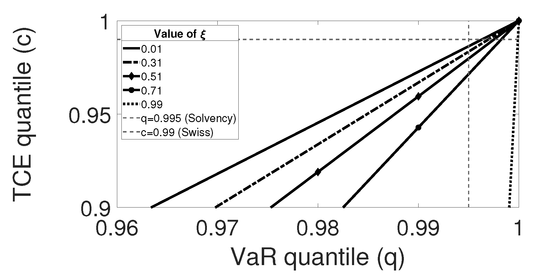
Figure 1. TCE quantile as a function of VaR quantile.
Risks 10 00142 g001
Figure 2. Extended TCE quantile as a function of VaR quantile. (Left panel): m = 2 and θ = 1 . (Right panel): m = 2 and θ = 5 .
Risks 10 00142 g002
Figure 3. Extended TCE quantile as a function of VaR quantile. (Left panel): m = 3 and θ = 1 . (Right panel): m = 3 and θ = 5 .
Risks 10 00142 g003
Figure 4. Extended TCE quantile as a function of VaR quantile. (Left panel): m = 2 , σ = 0.1 , and μ = 0.05 . (Right panel): m = 2 , σ = 0.1 , and μ = + 0.05 .
Risks 10 00142 g004
Figure 5. Extended TCE quantile as a function of VaR quantile. (Left panel): m = 2 , σ = 0.1 , and μ = 0 . (Right panel): m = 2 , σ = 0.4 , and μ = 0 .
Risks 10 00142 g005
Figure 6. Extended TCE quantile as a function of VaR quantile. (Left panel): m = 3 , σ = 0.1 , and μ = 0 . (Right panel): m = 3 , σ = 0.4 , and μ = 0 .
Risks 10 00142 g006
Figure 7. Extended TCE quantile at order n = 2 as a function of extended TCE quantile at order m = 5 . (Left panel): θ = 1 . (Right panel): θ = 2 .
Risks 10 00142 g007
Figure 8. TCE quantile as a function of extended TCE quantile at order 2. (Left panel): θ = 1 . (Right panel): θ = 2 .
Risks 10 00142 g008
Figure 9. Extended TCE quantile at order n = 2 as a function of extended TCE quantile at order m = 5 with σ = 0.1 . (Left panel): μ = 0.05 . (Right panel): μ = + 0.05 .
Risks 10 00142 g009
Figure 10. Extended TCE quantile at order n = 2 as a function of extended TCE quantile at order m = 5 with μ = 0 . (Left panel): σ = 0.1 . (Right panel): σ = 0.4 .
Risks 10 00142 g010
Figure 11. TCE quantile as a function of extended TCE quantile at order m = 2 with σ = 0.1 . (Left panel): μ = 0.05 . (Right panel): μ = + 0.05 .
Risks 10 00142 g011
Figure 12. TCE quantile as a function of extended TCE quantile at order m = 2 with μ = 0 . (Left panel): σ = 0.1 . (Right panel): σ = 0.4 .
Risks 10 00142 g012
Figure 13. Extended TCE quantile, with m = 2 , as a function of VaR.
Risks 10 00142 g013
Publisher’s Note: MDPI stays neutral with regard to jurisdictional claims in published maps and institutional affiliations.