Claims Modelling with Three-Component Composite Models


1
Department of Econometrics and Business Statistics, Monash University, Melbourne 3800, Australia
2
Research School of Finance, Actuarial Studies & Statistics, Australian National University, Canberra 0200, Australia
*
Author to whom correspondence should be addressed.
Risks 2023, 11(11), 196; https://doi.org/10.3390/risks11110196
Submission received: 28 September 2023
/
Revised: 29 October 2023
/
Accepted: 8 November 2023
/
Published: 13 November 2023
Abstract
:In this paper, we develop a number of new composite models for modelling individual claims in general insurance. All our models contain a Weibull distribution for the smallest claims, a lognormal distribution for the medium-sized claims, and a long-tailed distribution for the largest claims. They provide a more detailed categorisation of claims sizes when compared to the existing composite models which differentiate only between the small and large claims. For each proposed model, we express four of the parameters as functions of the other parameters. We fit these models to two real-world insurance data sets using both maximum likelihood and Bayesian estimation, and test their goodness-of-fit based on several statistical criteria. They generally outperform the existing composite models in the literature, which comprise only two components. We also perform regression using the proposed models.
1. Introduction
1.1. Current Literature
Modelling individual claim amounts which have a long-tailed distribution is an important task for general insurance actuaries. The usual candidates with a heavy tail include the two-parameter Weibull, lognormal, Pareto, and three-parameter Burr models (e.g., Dickson 2016). Venter (1983) introduced the four-parameter generalised beta type-II (GB2) model, which nests more than 20 popular distributions (e.g., Dong and Chan 2013) and can provide more flexibility in describing the skewness and kurtosis of the claims. McNeil (1997) applied the generalised Pareto distribution (GPD) to the excesses above a high threshold based on the extreme value theory. Many advanced models have been built with these various distribution assumptions, as it is crucial for an insurer to provide an adequate allowance for potential adverse financial outcome.
In order to deliver a reasonable parametric fit for both smaller claims and very large claims, Cooray and Ananda (2005) constructed the two-parameter composite lognormal-Pareto model. It is composed of a lognormal density up to an unknown threshold and a Pareto density beyond that threshold. Using a fire insurance data set, they demonstrated a better performance by the composite model when compared to traditional models like the gamma, Weibull, lognormal, and Pareto. Scollnik (2007) improved the lognormal-Pareto model by allowing the weights to vary and also introduced the lognormal-GPD model, in which the tail is modelled by the GPD instead. By contrast, Nadarajah and Bakar (2014) modelled the tail with the Burr density. Scollnik and Sun (2012) and Bakar et al. (2015) further tested several composite models which use the Weibull distribution below the threshold and a variety of heavy-tailed distributions above the threshold. In all these extensions, an important feature is that the threshold selection is based on the data. Moreover, all the authors hitherto imposed continuity and differentiability conditions on the threshold point, and so the effective number of parameters is reduced by two. While there are some other similar mixture models (e.g., Calderín-Ojeda and Kwok 2016; Reynkens et al. 2017) in the literature, we preserve the term “composite model” for only those with these continuity-differentiability requirements in this paper. Some other recent and related studies include those of Laudagé et al. (2019), Wang et al. (2020), and Poufinas et al. (2023).
1.2. Proposed Composite Models
All the composite models mentioned above have only two components. For a very large data set, the behaviour of claims of different sizes may differ vastly, which would then call for a finer division between the claim amounts and thus more components to be incorporated (e.g., Grün and Miljkovic 2019). In this paper, we develop new three-component composite models with an attempt to provide a better description of the characteristics of different data ranges. Each of our models contains a Weibull distribution for the smallest claims, a lognormal distribution for the medium-sized claims, and a heavy-tailed distribution for the largest claims. We choose the sequence of starting with the Weibull and then lognormal for a few reasons. First, as shown in Figure 1, the Weibull distribution tends to have a more flexible shape on the left side, which makes it potentially more useful for the smallest claims. Second, the lognormal distribution usually has a heaver tail, given the mean and variance, as the limiting density ratio of Weibull to lognormal approaches zero when goes to infinity (see Appendix A). This means that the lognormal distribution would be more suitable for claims of larger sizes. Nevertheless, both the Weibull and lognormal do not really possess a sufficiently heavy tail for modelling the largest claims. Comparatively, a heavy-tailed distribution like Pareto, Burr, and GPD are better options for this purpose. We apply the proposed three-component composite models to two real-world insurance data sets and use both maximum likelihood and Bayesian methods to estimate the model parameters for comparison. Based on several statistical tests on the goodness-of-fit, we find that the new composite models outperform not just the traditional models but also the earlier two-component composite models. In particular, it would be informative to see how the fitted models indicate the splits or thresholds to separate different claim sizes into three categories: small, medium, and large. We experiment with applying regression under the proposed model structure and realise that different claims sizes have different significant covariates. Moreover, we consider a 3D map which can serve as a risk management tool and summarise the entire model space and their resulting tail risk estimates. Note that we focus on the claim severity (but not the claim frequency) in this study.
The remainder of the paper is as follows. Section 2, Section 3 and Section 4 introduce the composite Weibull-lognormal-Pareto, Weibull-lognormal-GPD, and Weibull-lognormal-Burr models. Section 5 provides a numerical illustration using two insurance data sets of fire claims and vehicle claims. Section 6 sets forth the concluding remarks. The Appendix A presents some JAGS (specific software for Bayesian modelling) outputs of Bayesian simulation for the proposed models.
2. Weibull-Lognormal-Pareto Model
Suppose is a random variable with probability density function (pdf)
where
In effect, is the pdf of for , is the pdf of for and , and is the pdf of for , where ϕ, τ, μ, σ, and α are the model parameters. The weights and decide the total probability of each segment. The thresholds and are the points at which the Weibull and lognormal distributions are truncated, and they represent the splitting points between the three data ranges. We refer to this model as the Weibull-lognormal-Pareto model.
In line with previous authors including Cooray and Ananda (2005), two continuity conditions and , and also two differentiability conditions and are imposed at the two thresholds. It can be deduced that the former leads to the two equations below for the weights:
and that the latter generates the following two constraints:
Because of these four relationships, there are effectively five unknown parameters, including , , , , and , with the others , , , and expressed as functions of these parameters. As in all the previous works on composite models, the second derivative requirement is not imposed here because it often leads to inconsistent parameter constraints. One can readily derive that the kth moment of is given as follows (see Appendix A):
in which is the lower incomplete gamma function and .
3. Weibull-Lognormal-GPD Model
Similarly, we construct the Weibull-lognormal-GPD model as
Note that we use the GPD version as in Scollnik (2007), and that . Under the continuity and differentiability conditions, the weights are determined as follows:
and there are also two other constraints:
There are six effective model parameters of , , , , , and , with the others , , , and given as functions of these parameters. The kth moment of is equal to
where is the moment-generating function of the GPD, and is its kth derivative with respect to at for .
4. Weibull-Lognormal-Burr Model
Lastly, we define the Weibull-lognormal-Burr model as
For , the Burr distribution is truncated from below. Again, the continuity and differentiability conditions lead to the following equations for the weights:
and also the constraints below:
There are effectively seven model parameters to be estimated, including , , , , , , and . The others , , , and are derived from these parameters. The kth moment of is computed as
in which is the incomplete beta function.
Figure 2 gives a graphical illustration of the three new composite models. All the graphs are based on the values of and , that is, the expected proportions of small, medium, and large claims are 20%, 60%, and 20%, respectively. For illustration purposes, the parameters are arbitrarily chosen such that each set gives rise to exactly the same expected proportions of the three claim sizes. For the case in the top panel, which has similar Weibull and lognormal parameters and the same weights amongst the three models, the Pareto tail is heavier than the GPD tail, followed by the Burr one. In the bottom panel, while all the three Weibull-lognormal-Pareto models have the same component weights, the differences in the parameter values can generate very different shapes and tails of the densities. The three-component composite models can provide much flexibility for modelling individual claims of different lines of business.
5. Application to Two Data Sets
We first apply the three composite models to the well-known Danish data set of 2492 fire insurance losses (in millions of Danish Krone; a complete data set). The inflation-adjusted losses in the data range from 0.313 to 263.250 and are collected from the “SMPracticals” package in R. This data set has been studied in earlier works on composite models, including those of Cooray and Ananda (2005), Scollnik and Sun (2012), Nadarajah and Bakar (2014), and Bakar et al. (2015). For comparison, we also apply the Weibull, lognormal, Pareto, Burr, GB2, lognormal-Pareto, lognormal-GPD, lognormal-Burr, Weibull-Pareto, Weibull-GPD, and Weibull-Burr models to the data. Based on the reported results from the authors mentioned above, the Weibull-Burr model has been shown to produce the highest log-likelihood value and the lowest Akaike Information Criterion (AIC) value for this Danish data set.
The previous authors mainly used the maximum likelihood estimation (MLE) method to fit their composite models. While we still use the MLE to estimate the parameters (with nlminb in R), we also perform a Bayesian analysis via Markov chain Monte Carlo (MCMC) simulation. More specifically, random samples are simulated from a Markov chain which has its stationary distribution being equal to the joint posterior distribution. Under the Bayesian framework, the posterior distribution is derived as . We perform MCMC simulations via the software JAGS (Just Another Gibbs Sampler) (Plummer 2017), which uses the Gibbs sampling method. We make use of non-informative uniform priors for the unknown parameters. Note that the posterior modes under uniform priors generally correspond to the MLE estimates. For each MCMC chain, we omit the first 5000 iterations and collect 5000 samples afterwards. Since the estimated Monte Carlo errors are all well within 5% of the sample posterior standard deviations, the level of convergence to the stationary distribution is considered adequate in our analysis. Some JAGS outputs of MCMC simulation are provided in the Appendix A. We employ the “ones trick” (Spiegelhalter et al. 2003) to specify the new models in JAGS. The Bayesian estimates provide a useful reference for checking the MLE estimates. Despite the major differences in their underlying theories, their numerical results are expected to be reasonably close here, as we use non-informative priors, leading to most of the weights being allocated to the posterior mean rather than the prior mean. Since the posterior distribution of the unknown parameters of the proposed models are analytically intractable, the MCMC simulation procedure is a useful method for approximating the posterior distribution (Li 2014).
Table 1 reports the negative log-likelihood (NLL), AIC, Bayesian Information Criterion (BIC), Kolmogorov-Smirnov (KS) test statistic, and Deviance Information Criterion (DIC) values1 for the 14 models tested. The ranking of each model under each test is given in brackets, in which the top three performers are highlighted for each test. Overall, the Weibull-lognormal-Pareto model appears to provide the best fit, with the lowest AIC, BIC, and DIC values and the second lowest NLL and KS values. The second position is taken by the Weibull-lognormal-GPD model, which produces the lowest NLL and KS values and the second (third) lowest AIC (DIC). The Weibull-lognormal-Burr and Weibull-Burr models come next, each of which occupies at least two top-three positions. Apparently, the new three-component composite models outperform the traditional models as well as the earlier two-component composite models. The P–P (probability–probability) plots in Figure 3 indicate clearly that the new models describe the data very well. Recently, Grün and Miljkovic (2019) tested 16 × 16 = 256 two-component models on the same Danish data set, using a numerical method (via numDeriv in R) to find the derivatives for the differentiability condition rather than deriving the derivatives from first principles as in the usual way. Based on their reported results, the Weibull-Inverse-Weibull model gives the lowest BIC (7671.30), and the Paralogistic-Burr and Inverse-Burr-Burr models give the lowest KS test values (0.015). Comparatively, as shown in Table 1, the Weibull-lognormal-Pareto model produces a lower BIC (7670.88) and all the three new composite models give lower KS values (around 0.011), which are smaller than the critical value at 5% significance level, and imply that the null hypothesis is not rejected.
Table 2 compares the fitted model quantiles (from MLE) against the empirical quantiles. It can be seen that the differences between them are generally small. This result conforms with the P–P plots in Figure 3. Note that the estimated weights of the three-component composite models are about and . These estimates suggest that the claim amounts can be split into three categories of small, medium, and large sizes, with expected proportions of 8%, 54%, and 38%. For pricing, reserving, and reinsurance purposes, the three groups of claims may further be studied separately, possibly with different sets of covariates where feasible, as they may have different underlying driving factors (especially for long-tailed lines of business).
Table 3 lists the parameter estimates of the three-component composite models obtained from the MLE method and also the Bayesian MCMC method. It is reassuring to see that not only the MLE estimates and the Bayesian estimates but also their corresponding standard errors and posterior standard deviations are fairly consistent with one another in general. A few exceptions include and , which may suggest that these parameter estimates are not as robust and are less significant. This implication is in line with the fact that the Weibull-lognormal-GPD and Weibull-lognormal-Burr models are only the second and third best models for this Danish data set.
We then apply the 14 models to a vehicle insurance claims data set, which was collected from http://www.businessandeconomics.mq.edu.au/our_departments/Applied_Finance_and_Actuarial_Studies/research/books/GLMsforInsuranceData (accessed on 2 August 2020). There are 3911 claims in 2004 and 2005 ranging from $201.09 to $55,922.13. For computation convenience, we model the claims in thousand dollars. Table 4 shows that the Weibull-lognormal-GPD and Weibull-lognormal-Burr models are the two best models in terms of all the test statistics covered. They are followed by the Weibull-Burr and lognormal-Burr models, which produce the next lowest NLL, AIC, BIC, and DIC values. As shown in Table 5, the fitted model quantiles and the empirical quantiles are reasonably close under the two best models. It is noteworthy that the Weibull-lognormal-Pareto model ranks only about fifth amongst the 14 models. For this model, the computed second threshold () turns out to be larger than the maximum claim amount observed in the data. This implies that the Pareto tail part is not needed or preferred at all for the data under this model, and the fitted model effectively becomes a Weibull-lognormal model. By contrast, for the Weibull-lognormal-GPD and Weibull-lognormal-Burr models, the GPD and Burr tail parts are important components that need to be incorporated ( = 4.6 and 3.5). Similar observations can be made among the two-component models, in which the GPD and Burr tails are selected over the Pareto tail. The estimated weights of the best composite models are around and . Table 6 gives the parameter estimates of the three-component composite models, and again the MLE estimates and the Bayesian estimates are roughly in line.
Blostein and Miljkovic (2019) proposed a grid map as a risk management tool for risk managers to consider the trade-off between the best model based on the AIC or BIC and the risk measure. It covers the entire space of models under consideration, and allows one to have a comprehensive view of the different outcomes under different models. In Figure 4, we extend this grid map idea into a 3D map, considering more than just one model selection criterion. It can serve as a summary of the tail risk measures given by the 14 models being tested, comparing the tail estimates between the best models and the other models under two chosen statistical criteria. For both data sets, it is informative to see that the 99% value-at-risk (VaR) estimates are robust amongst the few best model candidates, while there is a range of outcomes for the other less than optimal models (the 99% VaR is calculated as the 99th percentile based on the fitted model). It appears that the risk measure estimates become more and more stable and consistent as we move to progressively better performing models. This 3D map can be seen as a new risk management tool and it would be useful for risk managers to have an overview of the whole model space and examine how the selection criteria would affect the resulting assessment of the risk. In particular, in many other modelling cases, there could be several equally well-performing models which produce significantly different risk measures, and this tool can provide a clear illustration for more informed model selection. Note that other risk measures and selection criteria than those in Figure 4 can be adopted in a similar way.
To our knowledge, regression has not been tested on any of the composite models so far in the actuarial literature. We now explore applying regression under the proposed model structure via the MLE method. Besides the claim amounts, the vehicle insurance claims data set also contains some covariates including the exposure, vehicle age, driver age, and gender (see Table 7). We select the best performing Weibull-lognormal-GPD model (see Table 4) and assume that , , and are functions of the explanatory variables, based on the first moment derived in Section 3. We use a log link function for and to ensure that they are non-negative, and an identity link function for 2. It is very interesting to observe from the results in Table 7 that different model components (and so different claim sizes) point to different selections of covariates. For the largest claims, all the tested covariates are statistically significant, in which the claim amounts tend to increase as the exposure, vehicle age, and driver age decrease, and the claims are larger for male drivers on average. By sharp contrast, most of these covariates are not significant for the medium-sized claims and also the smallest claims. The only exception is the driver age for the smallest claims, but its effect is opposite to that for the largest claims. These differences are insightful in the sense that the underlying risk drivers can differ between the various sources or reasons behind the claims, and it is very important to take into account these subtle discrepancies in order to obtain a more accurate price on the risk. A final note is that while remains about the same level after embedding regression, has increased to 0.734 (when compared to Table 6). The inclusion of the explanatory variables has led to a larger allocation to the Weibull component but a smaller allocation to the lognormal component.
As a whole, it is interesting to see the gradual development over time in the area of modelling individual claim amounts. As illustrated in Table 1 and Table 4, the simple models (Weibull, lognormal, Pareto) fail to capture the important features of the complete data set when its size is large. More general models with additional parameters and so more flexibility (Burr, GB2) are then explored as an alternative, which does bring some improvement over the simple models. The two-component composite lognormal-kind models represent a significant innovation in combining two distinct densities, though these models do not always lead to obvious improvement over traditional three- and four-parameter distributions. Later, some studies showed that two-component composite Weibull-, Paralogistic-, and Inverse-Burr-kind models can produce better fitting results. In the present work, we take a step ahead and demonstrate that a three-component composite model, with the Weibull for small claims, lognormal for moderate claims, and a heavy tail for large claims, can further improve the fitting performance. Moreover, based on the estimated parameters, there is a rather objective guide for splitting the claims into different groups, which can then be analysed separately for their own underlying features (e.g., Cebrián et al. 2003). This kind of separate analysis is particularly important for some long-tailed lines of business, such as public and product liability, for which certain large claims can delay significantly due to specific legal reasons. Note that the previous two-component composite models, when fitted to the two insurance data sets, suggest a split at around the 10% quantile, which is in line with the estimated values of reported earlier. The proposed three-component composite models can make a further differentiation between moderate and large claim sizes.
6. Concluding Remarks
We have constructed three new composite models for modelling individual claims in general insurance. All our models are composed of a Weibull distribution for the smallest claims, a lognormal distribution for the moderate claims, and a long-tailed distribution for the largest claims. Under each proposed model, we treat four of the parameters as functions of the other parameters. We have applied these models to two real-world insurance data sets of fire claims and vehicle claims, via both maximum likelihood and Bayesian estimation methods. Based on standard statistical criteria, the proposed three-component composite models are shown to outperform the earlier two-component composite models. We have also devised a 3D map for analysing the impact of selection criteria on the resulting risk measures, and experimented with applying regression under a three-component composite model, from which the effects of different covariates on different claim sizes are illustrated and compared. Note that inflation has been very high in recent years, and can have a serious impact on the claim sizes. Accordingly, it is advisable to adjust recent claim sizes with suitable inflation indices before the claims modelling, similar to the Danish data set.
There are a few areas that would require more investigation. For the two data sets considered, each of which has a few thousand observations, it appears that three distinct components are adequate to describe the major data patterns. For other much larger data sets, however, we conjecture that an incorporation of more than three components can become an optimal choice. Additionally, if the data set is sufficiently large, clustering techniques can be applied, and the corresponding results can be compared to those of the proposed approach. When clustering methods are used, the next step is to fit a distribution or multiple distributions to different claim sizes, while our proposed approach has the convenience of performing both in one single step. Moreover, we select the Weibull and then lognormal distributions because of their suitability for the smallest and medium-sized claims, as shown and discussed earlier, and the fact that they have been the common choices in the existing two-component composite models. While we use these two distributions as the base for the first two components, it may be worthwhile to test other distributions instead and see whether they can significantly improve the fitting performance. Finally, as in Pigeon and Denuit (2011), heterogeneity of the two threshold parameters can be introduced by setting appropriate mixing distributions. In this way, the threshold parameters are allowed to differ between observations. There are also other interesting and related studies such as those of Frees et al. (2016), Millennium and Kusumawati (2022), and Poufinas et al. (2023).
Author Contributions
Methodology, J.L. (Jackie Li) and J.L. (Jia Liu); Formal analysis, J.L. (Jackie Li) and J.L. (Jia Liu); Writing—original draft, J.L. (Jackie Li) and J.L. (Jia Liu). All authors have read and agreed to the published version of the manuscript.
Funding
This research received no external funding.
Data Availability Statement
The data used are publicly available, as in the links provided.
Conflicts of Interest
The authors declare no conflict of interest.
Appendix A
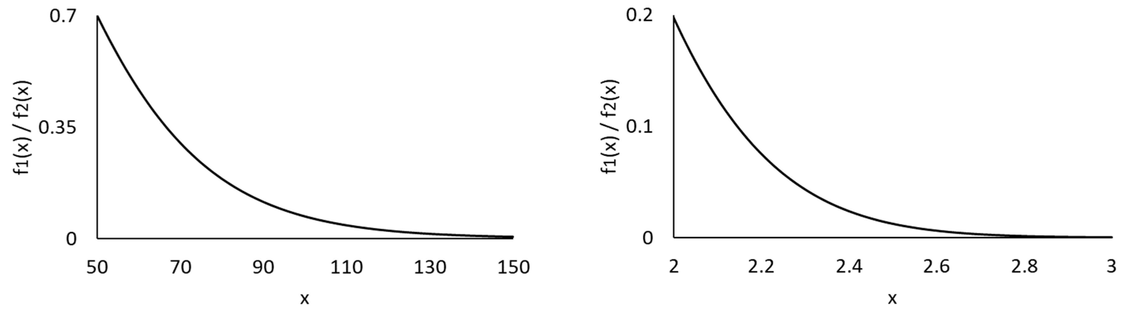
As shown in the example below, given the mean and variance, the limiting density ratio of Weibull to lognormal tends to zero when approaches infinity. This indicates that the lognormal distribution has a heaver tail than the Weibull distribution.
Figure A1.
Density ratios of Weibull (3.8511, 0.7717) to Lognormal (1, 1) (left graph) and Weibull (0.7071, 2) to Lognormal (−0.5881, 0.4915) (right graph).
Figure A1.
Density ratios of Weibull (3.8511, 0.7717) to Lognormal (1, 1) (left graph) and Weibull (0.7071, 2) to Lognormal (−0.5881, 0.4915) (right graph).
For the Weibull-lognormal-Pareto model, one can derive the kth moment of as below.
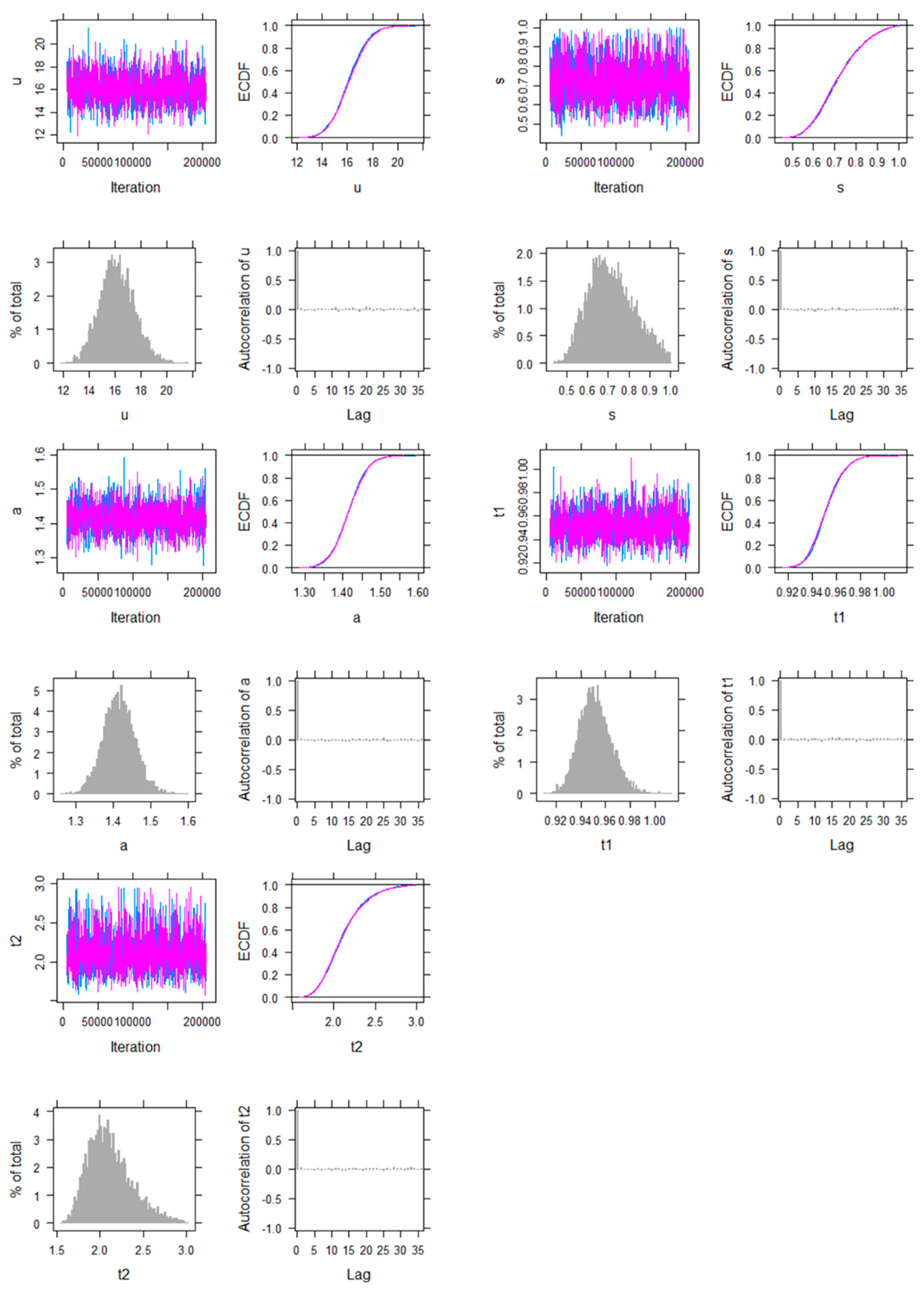
The following plots show the JAGS outputs of MCMC simulation when fitting the Weibull-lognormal-Pareto model to the Danish data, using uninformative uniform priors. All the parameters , , , , and are included. For each parameter, the four graphs include the history plot, posterior distribution function, posterior density function (in histogram), and autocorrelation plot (between iterations). The history and autocorrelation plots strongly suggest that the level of convergence to the underlying stationary distribution is highly satisfactory (Spiegelhalter et al. 2003).
Figure A2.
History plot, posterior distribution function, posterior density function, and autocorrelation plot of Weibull-lognormal-Pareto model parameters for Danish fire insurance claims data. (The blue and purple lines represent two separate chains of simulations.)
Figure A2.
History plot, posterior distribution function, posterior density function, and autocorrelation plot of Weibull-lognormal-Pareto model parameters for Danish fire insurance claims data. (The blue and purple lines represent two separate chains of simulations.)
| 1 | The AIC is defined as , and the BIC as , where is the computed maximum log-likelihood value, is the effective number of parameters estimated, and is the number of observations. The KS test statistic is calculated as , that is, the maximum distance between the empirical and fitted distribution functions. The DIC is computed as the posterior mean of the deviance plus the effective number of parameters under the Bayesian framework (Spiegelhalter et al. 2003). |
| 2 | The link functions are , , and , where ’s are the regression coefficients and , , , are the four covariates. We have checked the covariates in the data, and there is no multicollinearity issue. |
References
- Bakar, S. A. Abu, Nor A. Hamzah, Mastoureh Maghsoudi, and Saralees Nadarajah. 2015. Modeling loss data using composite models. Insurance: Mathematics and Economics 61: 146–54. [Google Scholar]
- Blostein, Martin, and Tatjana Miljkovic. 2019. On modeling left-truncated loss data using mixtures of distributions. Insurance: Mathematics and Economics 85: 35–46. [Google Scholar] [CrossRef]
- Calderín-Ojeda, Enrique, and Chun Fung Kwok. 2016. Modeling claims data with composite Stoppa models. Scandinavian Actuarial Journal 2016: 817–36. [Google Scholar] [CrossRef]
- Cebrián, Ana C., Michel Denuit, and Philippe Lambert. 2003. Generalized Pareto fit to the Society of Actuaries’ large claims database. North American Actuarial Journal 7: 18–36. [Google Scholar] [CrossRef]
- Cooray, Kahadawala, and Malwane M. A. Ananda. 2005. Modeling actuarial data with a composite lognormal-Pareto model. Scandinavian Actuarial Journal 2005: 321–34. [Google Scholar] [CrossRef]
- Dickson, David C. M. 2016. Insurance Risk and Ruin, 2nd ed. Cambridge: Cambridge University Press. [Google Scholar]
- Dong, Alice X. D., and Jennifer S. K. Chan. 2013. Bayesian analysis of loss reserving using dynamic models with generalized beta distribution. Insurance: Mathematics and Economics 53: 355–65. [Google Scholar] [CrossRef]
- Frees, Edward W., Gee Lee, and Lu Yang. 2016. Multivariate frequency-severity regression models in insurance. Risks 4: 4. [Google Scholar] [CrossRef]
- Grün, Bettina, and Tatjana Miljkovic. 2019. Extending composite loss models using a general framework of advanced computational tools. Scandinavian Actuarial Journal 2019: 642–60. [Google Scholar] [CrossRef]
- Laudagé, Christian, Sascha Desmettre, and Jörg Wenzel. 2019. Severity modeling of extreme insurance claims for tariffication. Insurance: Mathematics and Economics 88: 77–92. [Google Scholar] [CrossRef]
- Li, Jackie. 2014. A quantitative comparison of simulation strategies for mortality projection. Annals of Actuarial Science 8: 281–97. [Google Scholar] [CrossRef]
- McNeil, Alexander J. 1997. Estimating the tails of loss severity distributions using extreme value theory. ASTIN Bulletin 27: 117–37. [Google Scholar] [CrossRef]
- Millennium, Ratih Kusuma, and Rosita Kusumawati. 2022. The simulation of claim severity and claim frequency for estimation of loss of life insurance company. In AIP Conference Proceedings. College Park: AIP Publishing, vol. 2575. [Google Scholar]
- Nadarajah, Saralees, and SA Abu Bakar. 2014. New composite models for the Danish fire insurance data. Scandinavian Actuarial Journal 2014: 180–87. [Google Scholar] [CrossRef]
- Pigeon, Mathieu, and Michel Denuit. 2011. Composite lognormal-Pareto model with random threshold. Scandinavian Actuarial Journal 2011: 177–92. [Google Scholar]
- Plummer, Martyn. 2017. JAGS Version 4.3.0 User Manual. Available online: https://sourceforge.net/projects/mcmc-jags/files/Manuals/ (accessed on 1 November 2023).
- Poufinas, Thomas, Periklis Gogas, Theophilos Papadimitriou, and Emmanouil Zaganidis. 2023. Machine learning in forecasting motor insurance claims. Risks 11: 164. [Google Scholar] [CrossRef]
- Reynkens, Tom, Roel Verbelen, Jan Beirlant, and Katrien Antonio. 2017. Modelling censored losses using splicing: A global fit strategy with mixed Erlang and extreme value distributions. Insurance: Mathematics and Economics 77: 65–77. [Google Scholar] [CrossRef]
- Scollnik, David P. M. 2007. On composite lognormal-Pareto models. Scandinavian Actuarial Journal 2007: 20–33. [Google Scholar] [CrossRef]
- Scollnik, David PM, and Chenchen Sun. 2012. Modeling with Weibull-Pareto models. North American Actuarial Journal 16: 260–72. [Google Scholar] [CrossRef]
- Spiegelhalter, David, Andrew Thomas, Nicky Best, and Dave Lunn. 2003. WinBUGS User Manual. Available online: https://www.mrc-bsu.cam.ac.uk/software/bugs/ (accessed on 1 September 2023).
- Venter, Gary C. 1983. Transformed beta and gamma distributions and aggregate losses. Proceedings of the Casualty Actuarial Society 70: 156–93. [Google Scholar]
- Wang, Yinzhi, Ingrid Hobæk Haff, and Arne Huseby. 2020. Modelling extreme claims via composite models and threshold selection methods. Insurance: Mathematics and Economics 91: 257–68. [Google Scholar] [CrossRef]
Figure 1.
Examples of density functions of Weibull and lognormal distributions.

Figure 2.
Examples of density functions of three-component composite models with weights of 20%, 60%, and 20%, respectively.
Figure 2.
Examples of density functions of three-component composite models with weights of 20%, 60%, and 20%, respectively.
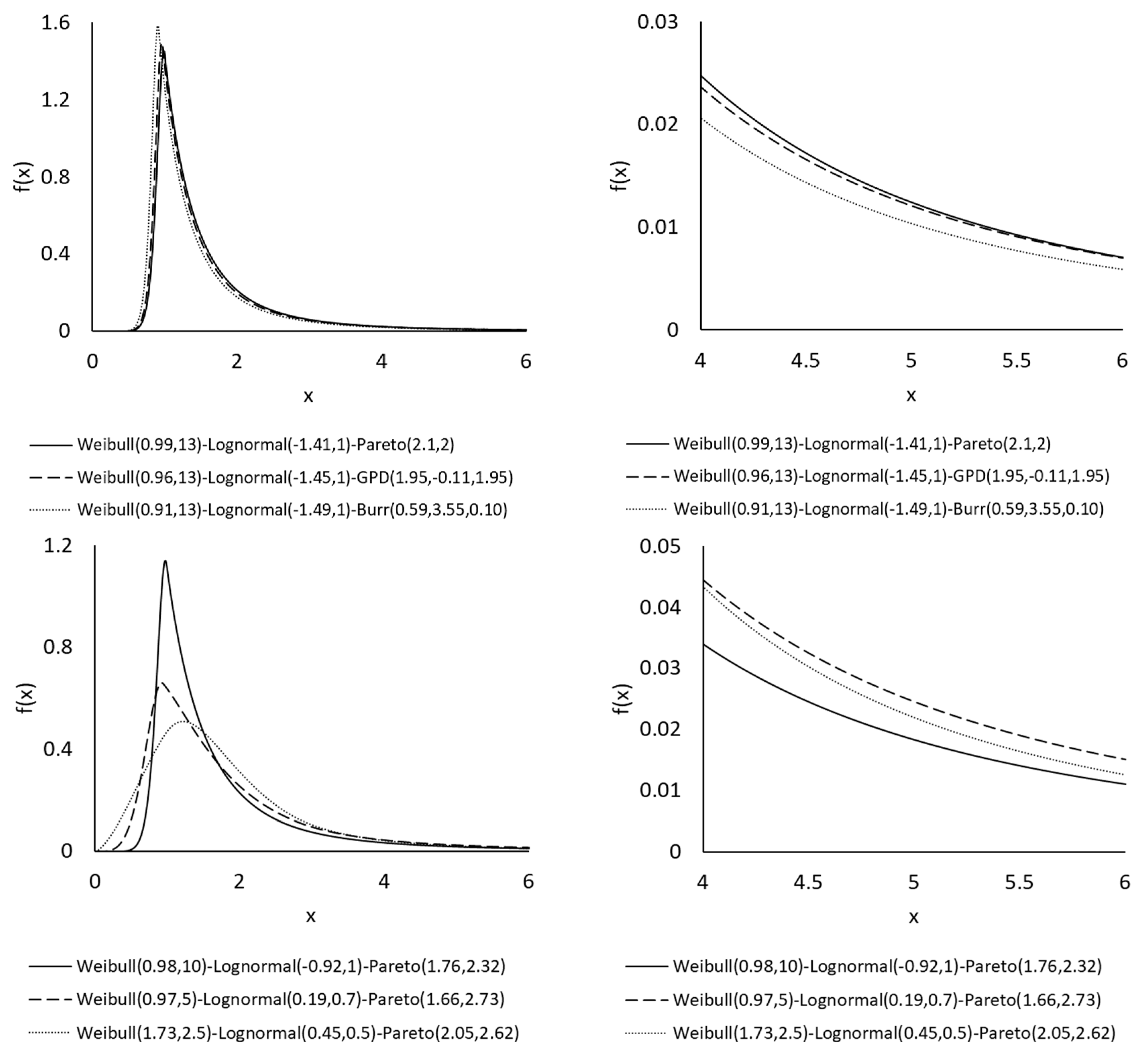
Figure 3.
P–P plots of fitting three-component composite models to Danish data.

Figure 4.
3D map of 14 models’ 99% VaR estimates against BIC and KS values for Danish fire insurance claims data (left) and vehicle insurance claims data (right). The three major categories are noted as traditional models (triangles), two-component composite models (empty circles), and new three-component composite models (solid circles).


Table 1.
Fitting performances of 14 models on Danish fire insurance claims data.
| Model | NLL | AIC | BIC | KS | DIC |
|---|---|---|---|---|---|
| Weibull | 5270.47 (14) | 10,544.94 (14) | 10,556.58 (14) | 0.2555 (13) | 33,495 (14) |
| Lognormal | 4433.89 (12) | 8871.78 (12) | 8883.42 (12) | 0.1271 (12) | 31,822 (12) |
| Pareto | 5051.91 (13) | 10107.81 (13) | 10119.45 (13) | 0.2901 (14) | 33,058 (13) |
| Burr | 3835.12 (7) | 7676.24 (6) | 7693.70 (6) | 0.0383 (9) | 30,625 (6) |
| GB2 | 3834.77 (6) | 7677.53 (7) | 7700.82 (7) | 0.0602 (11) | 30,626 (7) |
| Lognormal-Pareto | 3865.86 (11) | 7737.73 (11) | 7755.19 (11) | 0.0323 (8) | 30,687 (11) |
| Lognormal-GPD | 3860.47 (10) | 7728.94 (10) | 7752.23 (9) | 0.0196 (6) | 30,677 (10) |
| Lognormal-Burr | 3857.83 (9) | 7725.65 (9) | 7754.76 (10) | 0.0193 (5) | 30,673 (9) |
| Weibull-Pareto | 3840.38 (8) | 7686.75 (8) | 7704.21 (8) | 0.0516 (10) | 30,636 (8) |
| Weibull-GPD | 3823.70 (5) | 7655.40 (5) | 7678.68 (3) | 0.0255 (7) | 30,604 (5) |
| Weibull-Burr | 3817.57 (4) | 7645.14 (3) | 7674.24 (2) | 0.0147 (4) | 30,593 (4) |
| Weibull-Lognormal-Pareto | 3815.89 (2) | 7641.77 (1) | 7670.88 (1) | 0.0114 (2) | 30,589 (1) |
| Weibull-Lognormal-GPD | 3815.88 (1) | 7643.76 (2) | 7678.69 (4) | 0.0113 (1) | 30,590 (3) |
| Weibull-Lognormal-Burr | 3815.89 (3) | 7645.77 (4) | 7686.52 (5) | 0.0114 (3) | 30,590 (2) |
Note: We have checked some of these results against those reported in studies by Cooray and Ananda (2005), Scollnik and Sun (2012), Nadarajah and Bakar (2014), and Bakar et al. (2015), where available. We have also tested a wide range of initial values to obtain the most optimal MLE solutions.
Table 2.
Empirical and fitted composite model quantiles for Danish fire insurance claims data.
| Quantile | Empirical | Weibull-Lognormal-Pareto | Weibull-Lognormal-GPD | Weibull-Lognormal-Burr |
|---|---|---|---|---|
| 1% | 0.845 | 0.811 | 0.811 | 0.811 |
| 5% | 0.905 | 0.905 | 0.905 | 0.905 |
| 10% | 0.964 | 0.967 | 0.967 | 0.967 |
| 25% | 1.157 | 1.164 | 1.164 | 1.164 |
| 50% | 1.634 | 1.620 | 1.619 | 1.620 |
| 75% | 2.645 | 2.654 | 2.651 | 2.654 |
| 90% | 5.080 | 5.081 | 5.080 | 5.081 |
| 95% | 8.406 | 8.303 | 8.317 | 8.303 |
| 99% | 24.614 | 25.971 | 26.172 | 25.971 |
Note: The figures are produced from the authors’ calculations.
Table 3.
Parameter estimates of fitting three-component composite models to Danish fire insurance claims data.
Table 3.
Parameter estimates of fitting three-component composite models to Danish fire insurance claims data.
| Model | Maximum Likelihood | Bayesian MCMC (Posterior Distribution) | |||
|---|---|---|---|---|---|
| Estimate | Standard Error | Mean | Median | Standard Deviation | |
| Weibull-Lognormal-Pareto | τ = 16.253 | 1.290 | 16.127 | 16.073 | 1.351 |
| σ = 0.649 | 0.089 | 0.716 | 0.705 | 0.110 | |
| α = 1.411 | 0.040 | 1.416 | 1.415 | 0.042 | |
| θ1 = 0.947 | 0.011 | 0.952 | 0.951 | 0.013 | |
| θ2 = 1.976 | 0.189 | 2.113 | 2.078 | 0.254 | |
| Weibull-Lognormal-GPD | τ = 16.252 | 1.289 | 16.165 | 16.101 | 1.373 |
| σ = 0.648 | 0.088 | 0.728 | 0.719 | 0.113 | |
| α = 1.402 | 0.097 | 1.440 | 1.432 | 0.096 | |
| λ = −0.018 | 0.174 | 0.041 | 0.034 | 0.178 | |
| θ1 = 0.947 | 0.011 | 0.952 | 0.951 | 0.013 | |
| θ2 = 1.988 | 0.218 | 2.106 | 2.070 | 0.291 | |
| Weibull-Lognormal-Burr | τ = 16.253 | 1.290 | 16.14 | 16.106 | 1.376 |
| σ = 0.649 | 0.089 | 0.725 | 0.718 | 0.113 | |
| α = 0.449 | 1.575 | 0.526 | 0.477 | 0.193 | |
| γ = 3.143 | 1.015 | 3.069 | 2.994 | 1.010 | |
| β = 0.001 | 0.039 | 0.391 | 0.358 | 0.260 | |
| θ1 = 0.947 | 0.011 | 0.952 | 0.951 | 0.013 | |
| θ2 = 1.976 | 0.189 | 2.045 | 2.015 | 0.273 | |
Note: The figures are produced from the authors’ calculations.
Table 4.
Fitting performances of 14 models on vehicle insurance claims data.
| Model | NLL | AIC | BIC | KS | DIC |
|---|---|---|---|---|---|
| Weibull | 7132.74 (14) | 14,269.47 (14) | 14,282.02 (14) | 0.1414 (13) | 50,289 (14) |
| Lognormal | 6567.94 (12) | 13,139.87 (12) | 13,152.42 (12) | 0.0816 (5) | 49,160 (12) |
| Pareto | 6906.02 (13) | 13,816.03 (13) | 13,828.57 (13) | 0.1471 (14) | 49,836 (13) |
| Burr | 6292.07 (10) | 12,590.15 (10) | 12,608.96 (10) | 0.0911 (10) | 48,609 (10) |
| GB2 | 6300.41 (11) | 12,608.82 (11) | 12,633.90 (11) | 0.0783 (4) | 48,627 (11) |
| Lognormal-Pareto | 6281.18 (9) | 12,568.36 (9) | 12,587.17 (9) | 0.0934 (12) | 48,587 (9) |
| Lognormal-GPD | 6153.72 (7) | 12,315.43 (7) | 12,340.52 (7) | 0.0853 (8) | 48,333 (7) |
| Lognormal-Burr | 6076.13 (4) | 12,162.27 (4) | 12,193.62 (4) | 0.0766 (3) | 48,178 (4) |
| Weibull-Pareto | 6249.84 (8) | 12,505.67 (8) | 12,524.49 (8) | 0.0933 (11) | 48,524 (8) |
| Weibull-GPD | 6144.36 (6) | 12,296.72 (6) | 12,321.81 (6) | 0.0891 (9) | 48,314 (6) |
| Weibull-Burr | 6062.21 (3) | 12,134.43 (3) | 12,165.78 (3) | 0.0827 (7) | 48,150 (3) |
| Weibull-Lognormal-Pareto | 6088.95 (5) | 12,187.91 (5) | 12,219.27 (5) | 0.0822 (6) | 48,204 (5) |
| Weibull-Lognormal-GPD | 5971.78 (1) | 11,955.56 (1) | 11,993.19 (1) | 0.0764 (2) | 48,090 (2) |
| Weibull-Lognormal-Burr | 6025.74 (2) | 12,065.48 (2) | 12,109.38 (2) | 0.0743 (1) | 46,355 (1) |
Table 5.
Empirical and fitted composite model quantiles for vehicle insurance claims data.
| Quantile | Empirical | Weibull-Lognormal-Pareto | Weibull-Lognormal-GPD | Weibull-Lognormal-Burr |
|---|---|---|---|---|
| 1% | 0.234 | 0.250 | 0.250 | 0.252 |
| 5% | 0.338 | 0.318 | 0.314 | 0.317 |
| 10% | 0.354 | 0.361 | 0.353 | 0.358 |
| 25% | 0.440 | 0.510 | 0.493 | 0.496 |
| 50% | 1.045 | 0.964 | 0.961 | 0.968 |
| 75% | 2.560 | 2.257 | 2.346 | 2.473 |
| 90% | 5.813 | 5.464 | 5.762 | 5.711 |
| 95% | 8.993 | 9.600 | 8.852 | 8.887 |
| 99% | 18.845 | 28.889 | 18.167 | 18.842 |
Note: The figures are produced from the authors’ calculations.
Table 6.
Parameter estimates of fitting three-component composite models to vehicle insurance claims data.
Table 6.
Parameter estimates of fitting three-component composite models to vehicle insurance claims data.
| Model | Maximum Likelihood | Bayesian MCMC (Posterior Distribution) | |||
|---|---|---|---|---|---|
| Estimate | Standard Error | Mean | Median | Standard Deviation | |
| Weibull-Lognormal-Pareto | τ = 7.373 | 0.331 | 7.383 | 7.376 | 0.326 |
| σ = 1.789 | 0.047 | 1.797 | 1.795 | 0.063 | |
| α = 2.632 | 0.267 | 2.492 | 2.521 | 0.254 | |
| θ1 = 0.365 | 0.004 | 0.365 | 0.365 | 0.004 | |
| θ2 = 1312 | 1077 | 1054 | 1057 | 544 | |
| Weibull-Lognormal-GPD | τ = 7.707 | 0.304 | 7.856 | 7.851 | 0.244 |
| σ = 16.917 | 0.053 | 17.454 | 17.451 | 0.386 | |
| α = 4.483 | 0.016 | 4.428 | 4.428 | 0.039 | |
| λ = 12.717 | 0.054 | 12.444 | 12.443 | 0.122 | |
| θ1 = 0.366 | 0.003 | 0.357 | 0.357 | 0.003 | |
| θ2 = 4.626 | 0.033 | 4.699 | 4.699 | 0.093 | |
| Weibull-Lognormal-Burr | τ = 7.647 | 0.341 | 7.784 | 7.943 | 0.258 |
| σ = 12.401 | 0.210 | 12.392 | 12.288 | 0.231 | |
| α = 9.034 | 0.110 | 9.164 | 9.232 | 0.218 | |
| γ = 0.724 | 0.020 | 0.667 | 0.607 | 0.067 | |
| β = 35.198 | 0.371 | 35.297 | 35.595 | 0.514 | |
| θ1 = 0.367 | 0.004 | 0.366 | 0.366 | 0.003 | |
| θ2 = 3.538 | 0.092 | 3.683 | 3.848 | 0.255 | |
Note: The figures are produced from the authors’ calculations.
Table 7.
Parameter estimates and standard errors of fitting Weibull-lognormal-GPD regression model to vehicle insurance claims data with covariates.
Table 7.
Parameter estimates and standard errors of fitting Weibull-lognormal-GPD regression model to vehicle insurance claims data with covariates.
| Model Component | Covariate | Estimate | Standard Error | t-Ratio | p-Value |
|---|---|---|---|---|---|
| Weibull Component (small claims) | Intercept | 0.850 | 0.644 | 1.32 | 0.19 |
| Exposure | −0.085 | 0.055 | −1.54 | 0.12 | |
| Vehicle Age | 0.233 | 0.253 | 0.92 | 0.36 | |
| Driver Age | 1.921 | 0.013 | 143.55 | 0.00 | |
| Gender | −0.012 | 0.009 | −1.29 | 0.20 | |
| Lognormal Component (medium claims) | Intercept | −57.411 | 26.128 | −2.20 | 0.03 |
| Exposure | 8.179 | 26.821 | 0.30 | 0.76 | |
| Vehicle Age | 7.670 | 5.425 | 1.41 | 0.16 | |
| Driver Age | −5.023 | 4.670 | −1.08 | 0.28 | |
| Gender | −1.221 | 11.118 | −0.11 | 0.91 | |
| GPD Component (large claims) | Intercept | 2.269 | 0.192 | 11.80 | 0.00 |
| Exposure | −1.028 | 0.186 | −5.52 | 0.00 | |
| Vehicle Age | −0.116 | 0.043 | −2.71 | 0.01 | |
| Driver Age | −0.049 | 0.023 | −2.08 | 0.04 | |
| Gender | 0.275 | 0.074 | 3.72 | 0.00 |
Note: The figures are produced from the authors’ calculations.
Disclaimer/Publisher’s Note: The statements, opinions and data contained in all publications are solely those of the individual author(s) and contributor(s) and not of MDPI and/or the editor(s). MDPI and/or the editor(s) disclaim responsibility for any injury to people or property resulting from any ideas, methods, instructions or products referred to in the content. |
© 2023 by the authors. Licensee MDPI, Basel, Switzerland. This article is an open access article distributed under the terms and conditions of the Creative Commons Attribution (CC BY) license (https://creativecommons.org/licenses/by/4.0/).
Share and Cite
MDPI and ACS Style
Li, J.; Liu, J. Claims Modelling with Three-Component Composite Models. Risks 2023, 11, 196. https://doi.org/10.3390/risks11110196
AMA Style
Li J, Liu J. Claims Modelling with Three-Component Composite Models. Risks. 2023; 11(11):196. https://doi.org/10.3390/risks11110196
Chicago/Turabian StyleLi, Jackie, and Jia Liu. 2023. "Claims Modelling with Three-Component Composite Models" Risks 11, no. 11: 196. https://doi.org/10.3390/risks11110196
Note that from the first issue of 2016, this journal uses article numbers instead of page numbers. See further details here.