
Coupled Price–Volume Equity Models with Auto-Induced Regime Switching

1
Department of Mathematics, FCT NOVA, and Nova Math, New University of Lisbon, Quinta da Torre, 2829-516 Monte de Caparica, Portugal
2
Department of of Higher Mathematics, Don State Technical University, Gagarin Square 1, Rostov-on-Don 344000, Russia
3
Department of Data Analysis and Machine Learning, Financial University under the Government of the Russian Federation, Leningradsky Prospekt, 49, Moscow 125993, Russia
*
Author to whom correspondence should be addressed.
Risks 2023, 11(11), 203; https://doi.org/10.3390/risks11110203
Submission received: 6 October 2023
/
Revised: 11 November 2023
/
Accepted: 14 November 2023
/
Published: 17 November 2023
(This article belongs to the Special Issue Risks Journal: A Decade of Advancing Knowledge and Shaping the Future)
Abstract
:In this work, we present a rigorous development of a model for the Price–Volume relationship of transactions introduced in 2009. For this development, we rely on the precise formulation of diffusion auto-induced regime-switching models presented in our previous work of 2020. The auto-induced regime-switching models referred to may be based on a finite set of stochastic differential equations (SDE)—all defined on the same bounded time interval—and a sequence of interlacing stopping times defined by the hitting threshold times of the trajectories of the solutions of the SDE. The coupling between price and volume—which we take as a proxy of liquidity—is assumed to be the following: the regime switching in the price variable occurs at the stopping times for which there is a change of region—in the product state space of price and liquidity—for the liquidity variable (and vice versa). The regimes may be defined parametrically—that is, the SDE coefficients keep the same functional form but with varying parameters—or the functional form of the SDE coefficients may change with each regime. By using the same noise source for both the price and the liquidity regime-switching models—volume (liquidity), which, in general, is not a tradable asset—we ensure that despite incorporating information on liquidity, the price part of the coupled model can be assumed to be arbitrage free and complete, allowing the pricing and hedging of derivatives in a simple way.
Keywords:
regime switching diffusions; auto-induced regime switching diffusions; price; volume of transactions; liquidityMSC:
60H10; 60H35; 62M15; 62P20; 60J701. Introduction
Our goal in this work is to study a general model that could be used for pricing and hedging in an arbitrage free and complete financial market model, in which we can consider the mutual influence of the variations of volume—considered as a proxy of liquidity—in the variations of price and vice versa. We accomplish this desideratum with threshold-induced regime switching processes—both price and volume (liquidity) models will be regime switching process—but with a special coupling: the regime switch in the price process will occur at a random time when the volume process crosses a threshold and vice versa. We will show that despite its conceptual simplicity, this model can accommodate most of the usual scenarios describing the mutual influence of liquidity—quantified by the volume of transactions per unit of time—upon price (and vice versa). We will first describe the characteristics of a model of a pair of threshold-induced regime switching processes and we will prove the existence and unicity in law of such a pair of processes.
It is difficult to produce a precise definition of liquidity in financial markets that can account for all the properties that should be attributed to such a concept. Usual quantitative proxies for liquidity are the bid–ask spread —which is the difference between the offer and demand prices—and the number of shares traded by unit of time, which is, for us, the volume of transactions per unit of time. Both these proxies are nonnegative, and we will also suppose that, in our model, the liquidity process has as a state space.
We now briefly describe the contents of the present work.
- In Section 2, we provide an extensive literature review mainly focusing on several ways of considering liquidity in financial markets that are relevant to our purposes.
- Section 3 describes a joint model for price and liquidity—in our approach, liquidity will be taken as the volume of transactions per unit of time per day, in the subsequent practical application—as a regime switching system of SDE with the coefficients of the price model process switching as a consequence of the threshold crossing of the trajectory of the liquidity process and vice versa. We consider a series of plausible scenarios for the joint evolution dynamics of price and liquidity and we stress the need of considering double thresholds in order to prevent ambiguity in the definition of the threshold crossing stopping time.
- In Section 4, we prove the existence of the regime switching coupled (Price, Volume) process by means of the Yamada–Watanabe theorem. The regime switching coupled (Price, Volume) process is defined by gluing together trajectories of price and volume processes at random points defined by the threshold crossings.
- Section 5 is the first section on the application part of this work. We consider data from the Ford Motor Company and we present and justify the use of the Ornstein–Uhlenbeck model for the liquidity (volume) by resorting to observed characteristics of the data and the expected properties of the observed time series volume of transactions per unit of time.
- Finally in Section 7, we summarize the main results of this work and we project further studies that seem justified by the obtained results.
2. A Dedicated Literature Review
There is a vast amount of literature on the subject of liquidity in financial markets. We will first address some of the main aspects of liquidity in relation to our own work.
- Liquidity as a measure of easiness to convert assets into cash;
- The influence of liquidity in portfolio performance;
- Liquidity and the its bid–ask spread proxy;
- Liquidity and its volume of transactions proxy.
In the second part of this literature review, we will describe the works related to the main modeling tool in this work, the auto-induced regime switching stochastic processes given as solutions of stochastic differential equations (SDE). The following research papers deal with particular interpretations of liquidity more related to the easiness of conversion of assets into cash. In Kontŭs and Mihanović (2019), the authors considered liquidity level measured by cash to current liabilities ratio and a deterministic arithmetic mathematical model, for calculating net earnings through decreasing the amount of liquid assets. The work by Georgescu et al. (2020) introduced an analytical framework in their methodology to identify vulnerabilities arising from the liquidity and funding profiles of banks. They proposed a novel liquidity metric that gauges the stress factor necessary for banks to become illiquid, and they outlined another analytical framework for evaluating the resilience of banks in the face of a liquidity shock. The study assessed the impact on the liquidity position of individual banks, considering factors such as the magnitude of funding freezes and the availability of liquidity buyers, across different scenarios. Liquidity is defined as the ease of converting assets into cash without incurring fiscal penalties. In Dolfin et al. (2021), the authors employed the Kinetic Theory for Active Particles approach to simulate the dynamics of liquidity profiles within a complex adaptive network system resembling a stylized financial market. By tracking the time evolution of the aggregate degree of connectivity, they were able to assess the changing network efficiency in two distinct scenarios. This provided an initial analysis of the stability of the emerging and evolving network structures.
In the particular area of studies relating the influence of liquidity in portfolio performance, we may look to the following. A general review of several models of liquidity and issues related to liquidity, including price impact models with price manipulation strategies, was given in Gökay et al. (2011) in the collection Di Nunno and Øksendal (2011). A technical introduction to several aspects of the use of mathematical tools in the study of market liquidity is given in Guéant (2016). We stress the important statement of the author that option pricing models that consider liquidity issues are rarely utilized, mainly due to their predominantly nonlinear nature. Moreover, the author points out that nonlinear pricing models are troublesome in practice when dealing with a book of options. However, the author also stresses that managing options with significant nominal values, particularly when handled independently, underscores the importance of liquidity (see (Guéant 2016, p. 171)). In the work by Çetin and Rogers (2007), dealing with discrete time models, the authors adopted a contrary assumption from the assumptions we postulate in this work; the actions of agents only impact prices during their trading activities, leading to a price process for the share that remains unaffected by the agents’ actions at other times. Both the two following works study diffusion models for the price dynamics where the indirect feedback effect is modeled by making the drift and volatility coefficients depend on the large trader’s trading strategy. In the work by Cvitanić and Ma (1996), we can find the important idea that in the context of a generalized Black–Scholes model, hedging contingent claims involve incorporating coefficients in the stock price dynamics that explicitly rely on the wealth and portfolio process of a specific investor. In other words, the actions of a significant investor influence the price dynamics of primary securities. The paper by Cuoco and Cvitanić (1998) investigates the optimal consumption and investment challenge for an investor of large sums, whose portfolio decisions impact the instantaneous expected returns on the traded assets.
We now detail the analysis of some research papers that sheds light over the complex relations between liquidity assessed by the bid–ask spread and the activity of the market given by the volume of transactions. In the work by Johnson (2008), we learn that in a static perspective, the findings reported in the literature say that stocks that are traded more frequently tend to exhibit narrower bid–ask spreads. In contrast, in a dynamic perspective, when resorting to the statistical analysis of market data, increased trading volume does not necessarily result in markets being more liquid. The authors proposed the conciliation of these two perspectives by reporting an analysis which found that in the model, volume and liquidity are behaving independently, but volume is positively correlated with the liquidity variance, which can be taken as the liquidity risk. The interesting viewpoint that the actions of a fairly large trader can influence the price, causing a noticeable price impact, is taken in Glover et al. (2010); as a consequence, the price impact can be regarded as lasting, as it will impact the underlying price dynamics for other participants in the market. The authors consider a modified geometric Brownian model (GBM) for the stock price; the modification is taken in the volatility term in the associated PDE and is interpreted as the additional shares traded as a result of a deterministic hedging strategy, coupled with a function that models the form of price impact. The thorough analysis of PDE shows that the financial modeling in this equation is insufficient to describe the true price dynamics, thus opening the door to other approaches. In Liu and Yong (2005), the authors investigated how the price impact in the underlying asset market influences the replication of a European contingent claim, deriving a generalized partial differential equation (PDE) for Black–Scholes pricing and confirming the existence and uniqueness of a classical solution to this PDE. Their findings hold significant consequences for empirical statistical analysis of the volatility smile. Numerical analysis of the Black–Scholes type of a PDE obtained when liquidity constraints are introduced in the model are presented in Casabán et al. (2011); Company et al. (2010, 2012).
We will now discuss some relevant literature on volume of transactions and its interplay with price movements in order to establish the desired connection of volume of transactions as a proxy of liquidity of stock prices and, most importantly, to enlighten our model choices. The article by Ying (1966) provides an empirical analysis of the connection between stock prices—daily closing prices—and daily volume of transactions, using statistical tools. The author’s ideas on the connection price–volume is perfectly captured in the following statement: “Prices and volumes of sales in the stock market are joint products of a single market mechanism, and any model that attempts to isolate prices from volumes or vice versa will inevitably yield incomplete if not erroneous results.” The more significant results being that a reduced volume typically coincides with a price decrease, while a substantial increase in volume is generally associated with either a significant price rise or a substantial price fall. The work by Epps (1975) also states that a well-known saying on Wall Street suggests that the trading volume (the number of shares traded) tends to be higher in bull markets and lower in bear markets. A remarkable finding of the author is that the ratio of volume to price change is higher for upticks than the absolute value of this ratio on downticks; he arrived at this conclusion using a two parameter portfolio selection model as a framework and a lognormal model for the end-of-period values. The research by Epps and Epps (1976) gives a continuation of Epps (1975) by modeling the change of the logarithm of price as a mixture distribution with transaction volume as the mixing variable. One of the most significant conclusions reached in this study is that the volume of transactions and the returns from one transaction to the next are correlated random variables. In the article by Tauchen and Pitts (1983), the authors deduced, based on economic theory, the joint probability distribution of both price change and trading volume over any time interval within the trading day. The revue article by Karpoff (1987) also contributed to the understanding of the price–volume relation, offering, among other contributions, the empirical finding that volume shows a positive correlation with the extent of price change and, in equity markets, with the price itself. One of the most significant findings in the study by Jones et al. (1994) is that almost all the information in the trading behavior of agents is encapsulated in the frequency of trades during a specific interval. The authors also advised that their findings indicate that theoretical models should incorporate both trade frequency and size of trades, that is, that the volume of transactions by unit of time is a variable to be considered in the models for the price–volume interaction. They also insisted that a more challenging endeavour might be to explicitly define scenarios where the number of trades encompasses all pertinent information for security pricing, since the size of the trades contains little or no additional information. Finally, in this short review of works on the interaction price and volume of transactions, we note that in the recent study by Dong and Tang (2023), the authors provided an SDE joint model for the price–liquidity relationship, in which the liquidity model is an Ornstein–Uhlenbeck SDE.
The auto-induced regime switching for processes defined as solutions of stochastic differential equations (SDE) has been studied under different perspectives; see Esquível et al. (2020) for a recent review, from which we extract some highlights presented next. Our contributions to the theme of auto-induced regime switching processes given as solutions of SDE started with the PhD thesis by Mota (2007), later exploited in a study already dealing with liquidity modeling, i.e., Rianço et al. (2009), as well as in Mota (2013), where a stock price model with two different mean reverting regimes was studied. A comprehensive study of a stock price regime switching geometric Brownian model was presented in Mota and Esquível (2014), with a detailed analysis of some more technical aspects in Esquível and Mota (2014), and a large comparative statistical study of the regime-switching model and the usual models in Mota and Esquível (2016). In Mota et al. (2021), there is a further exploration of auto-induced regime-switching models with varying functional forms for the coefficients of the SDE. Let us now detail the interactions of our contributions with other authors’ contributions.
In Lejay and Pigato (2017), the authors took a stochastic process model, of geometric Brownian motion functional form type with two regimes corresponding to two disjoint regions of the phase space defined by a threshold; a region for values grater or equal than the threshold and a region for values lesser than the threshold. The theory in Le Gall (1984) allowed the deduction of the existence result for such a model. The fitting of the model to data—the same 21 stock prices used in Esquível and Mota (2014)—was completed by means of the theory of occupation times and local times estimators. A comparison between the results in both Lejay and Pigato (2017) and Pigato (2019) and the results in Esquível and Mota (2014) obtained by different methods was presented in Lejay and Pigato (2019a); since the data were the same and both methods are equally sound, the results were shown to be in good agreement. Moreover, Lejay and Pigato (2019a) allowed the reader to differentiate between the two models, allowing, nevertheless, to detect the similarities. An important remark is that the two models are structurally different, since it appears impossible to describe the model in Lejay and Pigato (2019a) as a process obtained as a sum of excursions of two different geometric Brownian processes; the reason being the structure of the level sets of the geometric Brownian processes. Another approach in the same thematic is provided in Lejay and Pigato (2019b); the model is the same model as in Lejay and Pigato (2019a), but only the estimators for the drift, maximum likelihood estimators, are studied. The estimators for the volatility were given in Lejay and Pigato (2018).
3. The Coupled Price–Liquidity (Volume) Model
Following Rianço et al. (2009), we consider a price–liquidity coupled model with regimes and thresholds given, in a first approximation, by the following stochastic differential equations:
where and are Brownian processes with the following correlation matrix:
and are the drift coefficients of the SDE defining the dynamics of the price and liquidity, respectively, and and are the volatility coefficients of these SDE; these coefficients are supposed to satisfy regularity conditions to ensure the existence and unicity of solutions, conditions that will be detailed in Section 4. The lower and upper thresholds for the price and liquidity are denoted, respectively, by , for the price and , , for the liquidity.
Let us state two hypotheses that rule the regime changes according to the parameters and thresholds. The first hypothesis concerns the SDE for the process describing the time evolution of the price in Formula (1).
- A
- The interplay of the regimes and the thresholds, for the process , is given by the following relations satisfied by the parameter values, and consequently, the price drift coefficient:with a similar relation for the price volatility coefficient.
- B
- The interplay of the regimes and the thresholds for the process , that is, the liquidity process, is given by:with a similar relation for the liquidity volatility coefficient.
The general question of existence and unicity of such a couple of processes is answered in Theorem 5. First, let us gain some intuition on the general properties and modeling capabilities of such a pair of price–liquidity processes. Combining different signs for the drifts according to parameters this model allows for, at least, 16 scenarios, which we detail in Table 1, reproduced from Rianço et al. (2009).
For all these scenarios, we will suppose that for the subdomains defined by the product of the two closed intervals with extremities given by the thresholds, that is, , both price and liquidity have small tendencies with respect to the tendencies in the other subdomains. Of course, some of these scenarios may lack economic sense. Let us concentrate on the first scenario, which may be described in the following way:
- If the price becomes larger than the highest threshold, then liquidity has a tendency to increase;
- If the price becomes smaller than the lowest threshold, then liquidity has a tendency to decrease;
- If liquidity becomes larger than the highest threshold, then the price has a tendency to increase;
- If the liquidity becomes smaller than the lowest threshold, then the price has a tendency to decrease.
This scenario can be achieved with a price and volume combination such as , , and also , and with a liquidity combination such as , , and also:
In Figure 1, we depict an example of a possible evolution of the random process according to the choices corresponding to the first scenario.
Remark 1
(On the double line representation, in Figure 2 and Figure 3, of the thresholds of Figure 1). For reasons that have to do with the structure of level sets of continuous local martingales—see Esquível and Mota (2014) for a detailed explanation—the thresholds , , , and must be taken, in fact, as double thresholds of the form for , for , and for , for . We note that, in the applications of this model, both and are to be chosen small enough so that the units of the processes and —for instance, USD and number of shares traded by unit of time—are insensitive to quantities lesser than and . The rule for the process crossing one of the thresholds, let us say , is the following: in the case that, for some , we have , we consider that the process crosses (from below) at the first time that , that is, at the hitting time of the upper part of the double threshold ; the others cases follow the same principle.
Remark 2
(On the (Price, Volume) regime regions). With a nontrivial determination of the four thresholds , , , and , the state space is divided in nine different subdomains. With the rule for regime switching defined in Remark 1, the double thresholds define nine regions in the complement of the region B, in the state space, formed by the following bands:
where, in each one, a combination of (Price, Volume) regimes is perfectly defined. There is no defined combination of (Price, Volume) regimes in the regions inside each of the bands in B; this fact is evident when we consider the possibility of the (Price, Volume) process staying inside of, say, a Price band while crossing the Liquidity band or vice versa.
Remark 3
(On the regime switching stopping times). An observed possible trajectory of the process such as the one represented in Figure 1 shows that the regime switching occurs whenever this processes passes from one subdomain to another one by crossing one Price threshold or one Liquidity threshold or both thresholds at the same time. The case when crosses a threshold—either or —and does not cross a threshold and the case when crosses a threshold—either or —and does not cross a threshold define in clear way a stopping time according to the principles explained in the Remark 1. Now, considering the double thresholds, we observe that each of the nine subdomains has an exterior border and an interior border (see Figure 2 and Figure 3), and thus, considered the region regimes, explicited in Remark 2, the random time change for switching subdomains is the hitting time of the interior border of the arrival subdomain.
The case when the change in subdomains is such that both and cross one of their respective thresholds at random times, say and —according to the principles explained in the Remark 1— such that , which, for instance, happens at an intersection point of an horizontal and a vertical border of an interior region, is a random time at which both the Price process and the Volume process simultaneously change regimes.
The example of a possible trajectory given in Figure 2—without the details in crossing the double thresholds and in Figure 3 including the details in crossing the double thresholds—shows that since the liquidity threshold has been hit, at time , there is at that time a Price regime switch and then when the Price threshold is hit at time , there is at that random time a Liquidity regime switch. The two sequences of regime switching hitting thresholds stopping times one sequence for Price and another for Liquidity are, in this way, unambiguously defined.
4. On the Existence of a Regime Switching Process
We observe that, by definition, in Formulas (1)–(3), the process only depend on the process —additionally, the process only depends on the process —by means of the sequence of stopping times defined in Remarks 1, 2, and 3. This sequence of stopping times has realizations which are the interlacing of the two sequences of times; one sequence for the crossing of the Price threshold and the other for the crossing of the Volume threshold, with the possibility of equal values in the two sequences of numbers whenever corner hitting occurs. Thus, we can apply the results on the existence of regime switching diffusions developed in Esquível et al. (2020) to each one of the SDE equations in Formula (1) separately. For the reader’s convenience, we now provide, following Esquível et al. (2020), an updated version of context and results that allow to prove the existence of the regime switching process in question.
Let be a complete probability space with a right-continuous complete filtration on it. Let be the Borel -algebra on . For the essential notions pertaining to the subject of existence and unicity of solutions of SDE, the reader is referred to the masterful expositions of (Liptser and Shiryaev 2001, p. 132) and (Kallenberg 2002, pp. 412–26).
Definition 1
(Progressively measurable processes). A process is progressively measurable—with respect to —if for every the process is such that for every , we have that is measurable with respect to .
We observe that since sections of functions defined on a product measure space are measurable, a progressive measurable process is adapted to the filtration . Now, consider an SDE given by:
with a Brownian motion with respect to some filtration such that, almost surely, for all :
in order for the Lebesgue and Ito’s integrals implicit in Formula (5) to exist, and such that the integrands in Formula (5) are progressively measurable. For our purpose, we formulate a third hypothesis, where we will suppose that the stopping times of regime switching, of both price and liquidity, are satisfied.
- C
- Let be an increasing sequence of -stopping times, denoted by , such that we have, almost surely, and, for any , the function:is almost surely finite, that is, .
It is well known that pathwise uniqueness implies uniqueness in law (Proposition 1 in (Yamada and Watanabe 1971, p. 158) or Proposition 3.20 in (Karatzas and Shreve 1991, p. 309)). Furthermore, there is a remarkable result connecting strong existence and pathwise uniqueness due to Yamada and Watanabe Yamada and Watanabe (1971), which has a thorough treatment in (Kallenberg 2002, p. 424).
Theorem 1
(Strong solutions and pathwise uniqueness). Let an SDE—specified by its coefficients μ and σ—have weak solutions and pathwise uniqueness for a given initial law . Then, strong existence and uniqueness in law hold for such solutions.
Existence and unicity of SDE solutions can be studied in Braumann (2019) in the case of Lipschitz regularity and sublinear growth of the coefficients. For our purposes, we have the following important result, initially formulated for homogeneous SDE, that is also valid in the nonhomogeneous case (see (Rogers and Williams 2000, p. 266)). This result is essentially an existence and unicity in law of strong solutions of SDE with irregular coefficients. In (Prokhorov and Shiryaev 1998, p. 40) (and in (Karatzas and Shreve 1991, p. 291), with essentially the classical proof of the Yamada–Watanabe result), there is a formulation of Theorem 1 in (Yamada and Watanabe 1971, p. 164) for nonhomogeneous drift and volatilities that—for dimension one—suit better our purposes of having processes with continuous trajectories.
Theorem 2
(Yamada and Watanabe 1971). Suppose that μ and σ are progressively measurable and satisfy the following hypothesis.
- D
- There exists , an increasing continuous function possibly dependent of , such that , such that:and
- E
- There exists , an increasing concave function, possibly dependent of , such that , such that:and
Then, for any random variable Z, and , pathwise uniqueness holds for the following stochastic differential equation:
Remark 4.
Starting with Theorem 2, that is, the important Yamada–Watanabe result, we have, by the continuity of both μ and σ, applying a well known Skorokhod’s theorem (see (Kallenberg 2002, p. 419)) that there is a weak solution. Finally, by Theorem 1, strong existence and uniqueness in law holds.
The following result is proved in a more general context in Esquível et al. (2020). For the reader’s convenience, we present here a proof that applies directly to the SDE in Formula (1) and that we hope may enlighten the procedure of building a regime switching process by gluing excursions obtained as solutions of SDE.
Theorem 3
(On the existence of regime switching solutions to SDE). Consider a finite set as the parameters of the different m regimes. Let the functions and satisfy the hypothesis of Theorem 2. Let the increasing sequence of -stopping times , defined according to Remark 1, Remark 2, and Remark 3, verify hypothesis C. There exists a process , with continuous trajectories, which is a unique in law regime switching process associated with the parameter space Θ together with the increasing sequence of -stopping times .
Proof.
Consider some random variable measurable with respect to and consider the SDE given by:
where the functions and satisfy the hypothesis of Theorem 2 for every . We observe that the strong solution exists and is unique in law. Now, consider, after the regime switching at time , that the new value of the parameter is . Again, the SDE:
As before, the strong solution and unique in law solution exists and we may define . By induction, we may so have a sequence of unique in law processes and so—using the hypothesis of the sequence of stopping times stated in Formula (7),—we may define the process, for almost all :
which is the unique in law process obtained by gluing together excursions corresponding to regimes prescribed by the initially given sequence of stopping times. The proof that any excursion, for any possible value of the parameter, has a version that is almost surely continuous is a consequence of a general theorem on the dependence on parameter in (Kallenberg 2002, p. 345). This implies that the process has continuous trajectories. □
A simple condition in Theorem 4 ensures that the essential hypothesis on the sequence of stopping times is verified (see Esquível et al. (2020)).
Theorem 4
(A condition ensuring admissible sequence of stopping times). If σ is such that the Ito’s stochastic integral part in the SDE given by Formula (5) is a martingale then verifies Hypothesis C.
It is possible now to formulate a result that ensures the existence of the price–liquidity model proposed. In a first approach, since we want a complete model for pricing, we will suppose that the Brownian processes and are the same. For the general case, we have to state results with enlargement of filtrations corresponding to the two noise sources and .
Theorem 5
(On the existence of a price–liquidity process model). Suppose that for the SDE in Formula (1), both Hypothesis A and Hypothesis B are verified. Suppose that μ and σ—as well as ν and η—satisfy Hypothesis D and Hypothesis E. Suppose that the increasing sequence of -stopping times , derived as an application of Theorem 3 and of Remarks 1, 2 and 3, do satisfy hypothesis C. Then, there exists a unique in law regime switching process with continuous trajectories.
Proof.
The proof is a consequence of Theorem 3 applied to each one of the equations in Formula (1) with the sequence of stopping times generated by the procedure indicated in the Remarks 1, 2, and 3. □
5. Price and Liquidity Models
In the following, we consider particular examples of joint price and liquidity models in order to study real data and assess the functioning of the mixed regime-switching model introduced in Section 3 and studied in Section 4. We recall that our interpretation of liquidity is given by the volume of transactions, that is, the number of transactions by unit of time. We will first deal with the problem of adequately modeling liquidity.
5.1. Liquidity Models
First, let us explore two models for the liquidity as given by the volume of transactions. Let us detail some of the intrinsic and of the observable data characteristics of the daily number of transactions.
- As pointed out previously, there are connections between the variation of the price and a consequent variation of the volume of transactions and vice versa. We propose in this work a model to describe the aforementioned connections.
- The daily number of transactions reflects the available share of the public capital of the firm that integrates the portfolios of common investors. It is expected that the proportion of this public capital, with respect to the whole public capital of the firm, fluctuates around a certain value; this intrinsic characteristic points to a possible mean reverting model.
- There appear to exist abrupt and very significant changes on the volume of transactions that are not immediately connected to the information flow on the value of the firm that influences the price changes. This may occur caused by several reasons: sudden need for cash of an agent with a large share of the public capital of the firm (see, again, Çetin and Rogers (2007); Glover et al. (2010); Gökay et al. (2011), (Guéant 2016, p. 171)); some herd investment phenomena associated with the emergence of an independent and new more rewarding source of profit; and some herd investment phenomena associated with the disappearance of an independent and previously well established source of profit. This characteristic seems to justify the coupling of a mean reverting model with some jump process; we will not consider jump processes in this work.
These characteristics justify the research we present next. We will consider first the exponential Ornstein–Uhlenbeck (EOU) (see, for instance, Schwartz (1997)) given by:
which by Ito’s formula is seen to be the exponential of the well known Ornstein–Uhlenbeck diffusion process. That is, if , then , a very well-known process. In particular, the parameter estimation for such a process can be performed very efficiently (see Aït-Sahalia (2002)).
It is advisable to look at a paradigmatic dataset in order to get a general idea of some qualitative characteristics of a volume of transactions set. The dataset we will consider is from the Ford Motor Company stock and ranges from 19 March 2018 to 17 March 2023, roughly a five-year-long observation of the volume of transactions. In Figure 4, we present on the left-hand side the data and on the right-hand side a simulated trajectory of an exponential Ornstein–Uhlenbeck process with a set of parameters estimated by a heuristic method in such a way that the mean of the process coincides with the mean of the data. We considered the double logarithms of the volume of transactions data in order to lower the order of magnitude of the data—a desirable property for the estimation procedure—and in order to better accommodate the particular model chosen. In the data of this five-year-long set of daily observations, on the left-hand side of Figure 4, it is clear by inspection that there are several significant regime changes taking place around days 400, 500, and 600. It would be advisable to consider this extended period for the application of the joint regime-switching model of Section 3 and Section 4 if we want to find regime changes. At first sight, both the right-hand and the left-hand side of Figure 4 could be thought to be trajectories of the same process, that is, a first argument to support the adequateness of the model given in Formula (11).
5.2. Price Models
For the price model, we consider the classical geometrical Brownian model given by an SDE of the form:
This model was already considered in regime-switching models in Esquível and Mota (2014); Mota (2013) and provides excellent results with respect to pricing of derivatives.
6. Parameter Estimation
In this section, we develop a methodology for the estimation of the model thresholds and regime parameters. The main idea is to start with an equidistant Euler–Maruyama discretization of the SDE and to observe that the recurrence generated allows the definition of a conditional density that can be taken as a contrast quasi-likelihood. Starting references to this methodology are given in Pedersen (1995a, 1995b) and the methodology was exploited in the context of regime-switching models in Mota and Esquível (2016); Mota et al. (2021). An alternative way of building contrast functions that also produce consistent and asymptotically normal estimators is given in Kessler (1997).
6.1. On the Quasi-Likelihood Estimators
Let us briefly expose the general method to obtain estimators that maximize a quasi-likelihood function built upon the Euler–Maruyama discretisation of an SDE. Consider a process given as a solution of an SDE such as the following:
Under regularity conditions, this equation has a strong and unique solution (see (Øksendal 2003, p. 66)). Suppose that these conditions are verified and consider the Euler–Maruyama discretisation scheme given by:
which under regularity conditions—joint measurability of the coefficients, Lipschitz conditions, sublinear growth—is known to have a strong order of convergence of at least (see (Kloeden and Platen 1992, pp. 324–26)). The Euler–Maruyama in the form given by:
may be considered a recursive method for building the approximate trajectories of the solutions of the SDE. Considering the equidistant sequence of time points given by and observing that the increments of the Brownian process are normally distributed, which we denote by , we have that , the law of given that , is given by:
As a consequence, the conditional density of the law is given by:
From this conditional density, we may now assume that the density of the transition probability to go from to in time is given by:
Furthermore, as a consequence, using the Markov character of the process, the logarithm of the density of the transition probability to go from to in time :
In order to get a quasi-likelihood function that we can use as a contrast function, we may neglect the terms that do not contain the parameter functions and and we obtain the contrast quasi-likelihood function given by:
We now consider the particular cases that are relevant for our study. In case of the GBM and and thus, the contrast quasi-likelihood function— to be maximized—is given by:
By equating the derivative of to zero with respect to each of the parameters, we obtain the quasi-normal equations derived from the quasi-likelihood contrast function and we get the estimators in the usual way. The correspondent estimate for the parameter , obtained from the observed data , is given by:
and the estimate of the parameter is given by:
We now consider the model for the liquidity given by the volume of transactions. As previously observed, we want to model “ln(ln(Volume))” with an exponential Ornstein–Uhlenbeck (EOU) process . Then, with , that is with , we have that is an Ornstein–Uhlenbeck (OU) process. Thus, we must model “ln(ln(ln(Volume)))” by to have “ln(ln(Volume))” modeled by . In case of the OU process with and , we have:
The estimate of the parameter , obtained from the observed data , is given by:
the estimate of the parameter is given by:
and the estimate of the parameter is given by:
We observe that the estimates and are coupled in a system of equations that has to be solved as one.
The estimation procedure we use is similar to the one developed previously in Esquível and Mota (2014); Mota (2013); Mota and Esquível (2014); Mota et al. (2021), but adapted for the coupled model (Price, Volume) and is described next.
- We identify a domain of variation for the data and we choose accordingly two extreme values both for the thresholds of the price and the volume of transactions; an example of the criteria for the choice of the thresholds is to have at least ten observations above the upper threshold and ten observations below the lower threshold.
- For a given set of thresholds, we estimate the parameters and compute the value taken by the quasi-likelihood contrast functions on the estimated values of the parameters. The estimation of the parameters is done as follows. We consider the pairs (Price, Volume) for each date. We estimate three sets of the Price model parameters; the first set, with the Price data observations corresponding to the Volume observations that exceed the upper Volume threshold; the second set of parameters, with the Price data observations corresponding to the Volume observations in the region between the upper and the lower threshold; and the third set of parameters, with the Price data observations corresponding to the Volume observations in the region below the lower Volume threshold. We then estimate the three sets of Volume model parameters in a similar way as done with the Price parameter estimation but classifying the Volume data observations in three sets according to the positions of the corresponding Price observation with respect to the two thresholds: above the upper Price threshold, between the Price thresholds, and below the lower Price threshold.
- For the first round of research we reduce the difference between the lower and the upper threshold of both the Price and Volume data by a fixed quantity proportional to the initial separations between the thresholds. Furthermore, we repeat the parameter estimation procedure until the minimal distance between the thresholds—defined by the initial separation of thresholds divided by a fixed quantity—is attained. We identify the values of the thresholds corresponding to the maximum of the quasi-likelihood contrast function and, for the second round of research, we consider a neighborhood of the two sets of thresholds. We next proceed as in the first round and so on and so forth. After a finite number of rounds, the value of the quasi-likelihood contrast function is constant in an interval and we chose the thresholds corresponding to the middle point of this interval.
6.2. Parameter Estimation: Results and Interpretation
The results of the estimation procedure give the values below, with the increasing scale of importance of the values being: blue, orange, and red. The total number of observations considered was 1259.
The estimated thresholds—for and for —are the following: Volume: 2.92666, 2.84673; Price: 2.95864, 1.86765
Price parameters:
- INSIDE region to volume thresholds, − used observations: 988
- OUTER region to UPPER volume threshold, − observations used: 16
- OUTER region to LOWER volume threshold, − observations used: 67
Total observations used in the estimation: 1071 (85.1%)
Volume parameters:
- INSIDE region to price thresholds, , − observations used: 1110
- OUTER region to the UPPER price threshold, , − observations used: 57
- OUTER region to the LOWER price threshold, , − observations used: 79
Total observations used in the estimation: 1246 (98.9%).
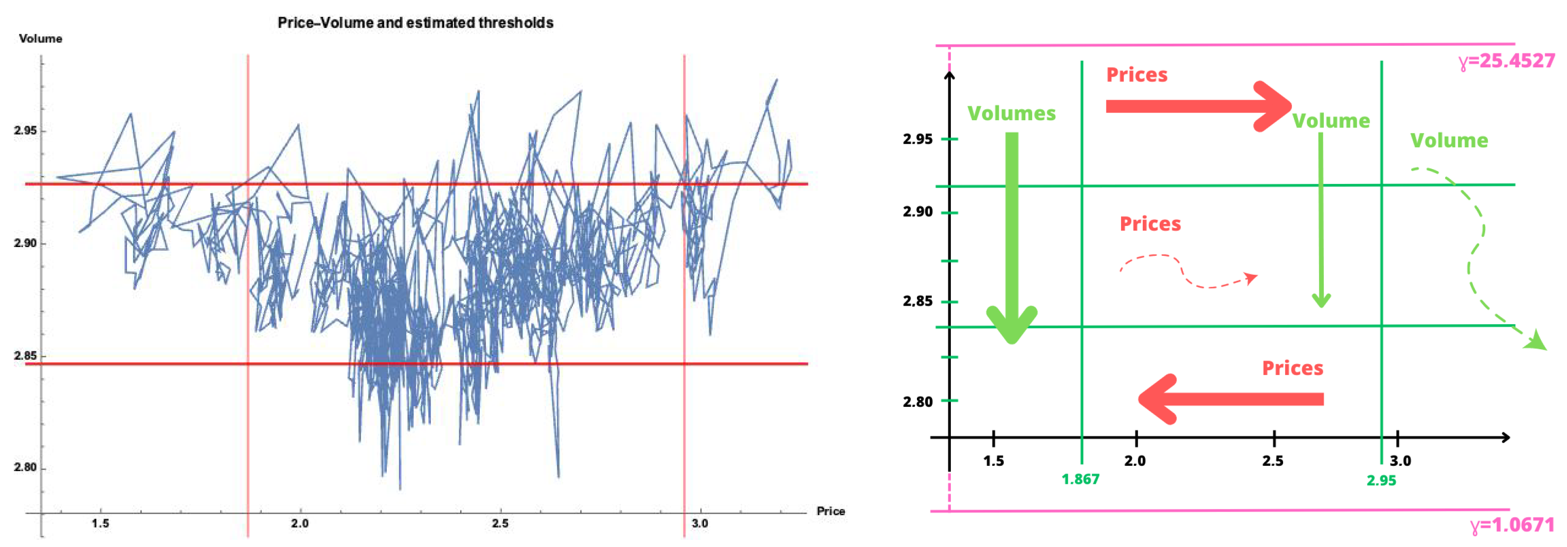
In Figure 5, we have, on the left-hand side, the observed trajectory (Price–Volume) and the estimated thresholds. By resorting to the SDE model estimated parameters, we can observe on the right-hand side of the figure a scheme of the (Price–Volume) dynamics in the phase space of the observed (Price–Volume) trajectory.
The (Price, Volume) dynamics—as analyzed with respect to the logarithm of price and the two-fold logarithm of volume—is different according to one of the nine regions defined by the two thresholds for the price and the two thresholds for the volume; the dynamics depend of the conjunction of the parameters that are different for each of the three regimes of Price and the three regimes of Volume, similarly to what is depicted in Figure 1.
On the right-hand side of Figure 5, we present a schematic representation in the phase space (Price, Liquidity) of the estimated parameters. The general principle for reading this representation is that a greater thickness of the arrow represents a larger value of the parameter and a wavy arrow represents a higher volatility. Furthermore, the direction of the arrow is self explicit: for price—in the horizontal axis of the phase space—since the model is the GMB process, it goes from right to left for a negative drift and it goes from left to right for a positive drift; for liquidity (volume of transactions)—in the vertical axis—the general tendency is decreasing, but this tendency is of different nature for prices lesser than the upper price threshold and for prices larger than this threshold.
In fact, for prices lesser than the upper price threshold, the volume mean reversion occurs in the direction of a value smaller than the values taken by the observed trajectory (Price,Volume). For prices larger than the upper price threshold, the volume mean reversion occurs in the opposite direction of a much larger value than the values taken by the observed trajectory (Price,Volume). The right-hand side of Figure 5 shows that the dynamics of the observed (Price,Volume) trajectory of the Ford Motor Company is of type IV, as defined in Table 1 of page 6. The behavior of the Ford Motor company stock depicted by this model clearly indicates that liquidity decreases in either the highest or the lowest prices and that prices tend to increase with higher liquidity and to decrease with the lowest liquidity; both these conclusions are coherent with standard economic considerations. Firstly, the highest or lowest prices will indicate a reversal of stock demand tendency, and secondly, higher liquidity (respectively, lower liquidity), indicating an increase in demand (respectively, a decrease in demand), will be accompanied by increasing prices (respectively, decreasing prices). At the managerial level of an investment company, admitting the stationarity hypothesis in the dynamics, that is, nonexistence of unexpected high impact events, this information has a clear use; for instance, if prices are at a high point level, high volume trades will face liquidity problems; for instance, at higher liquidity levels, buying may be advisable.
7. Conclusions and Further Work
In this work, we present a complementary study of a coupled regime-switching model for the Price and Volume of transactions—as a proxy of liquidity—of equities, previously introduced in Rianço et al. (2009). We show the existence of a stochastic process that satisfies the SDE equations for Price and Volume with coefficients switching according to thresholds crossing. The existence of this stochastic process comes from the existence of an increasing sequence of threshold hitting regime switching stopping times. In order to build this sequence, the first fundamental rule is that the regime only changes after the trajectory reaches the second threshold of a double line threshold. As a result, there is an increasing sequence of stopping times for Price and there is also a similar one for Volume; from the existence of these two sequences, we can infer that there is a sequence of increasing stopping times for regime switching that are stopping times either for Price regime switching or for Volume regime switching, being always possible to specify their respective nature in any realization of the sequence, that is, if it is a stopping time for Price regime switching or if it is a stopping time for Volume regime switching. These realizations are sequences, of real positive numbers, formed by intertwining times and there may be time values for which both trajectory of the processes, Price and Volume, change regime simultaneously.
We showed how to estimate both the parameters and the thresholds and we applied the estimation procedure introduced to a particular dataset providing an interpretation of the estimated values found in accordance with the model proposed. As a first line of future work, it would be interesting to compare the derivative pricing performance of the model here introduced to the performance of the price GBM regime-switching model in a study similar to the one in the study by Mota and Esquível (2014). Increased performance results for the (Price, Volume) regime-switching model would sustain the importance of considering the information gained by the volume of transactions.
Another natural and more general question to be studied is to model the price–volume relation in the context of algorithmic trading, a methodology that has been largely adopted in many stock exchanges.
A very interesting line of investigation is the auto-induced regime switching diffusions under the perspective of the theory of random dynamical systems. It is well known (see (Arnold 1998, pp. 473–75)) that if the coefficients of the SDE are smooth the Lyapunov exponent of the unique solution of the Fokker–Planck equation associated with the SDE is strictly negative, and hence, the random dynamical system generated by the SDE is exponentially stable. Since, at least in the application developed in this work, the solution of the auto-induced regime switching diffusion is obtained by the gluing of solutions of SDE with smooth coefficients (see Theorem 3), it follows that the regime switching stopping times may be considered as bifurcations points of the random dynamical system. The theory of bifurcations of random dynamical systems has made progress that are presented, for instance, in Crauel and Gundlach (1999).
As already pointed out in Esquível and Mota (2014), the auto-induced regime-switching models with one varying quantity—for instance, temperature—are adequate to describe, for instance, the functioning of a thermostat. The model described in this work with two mutually influencing varying quantities can be used to describe the behavior, for instance, of a hygrostat-thermostat device, which is a device that simultaneously regulate temperature and humidity. A consequent line of investigation is the possible application of the models developed here to other industry phenomena.
Author Contributions
Conceptualization, M.L.E.; methodology, M.L.E., N.P.K., P.P.M. and V.V.S.; software, M.L.E., N.P.K. and P.P.M.; validation, M.L.E., N.P.K., P.P.M. and V.V.S.; formal analysis, M.L.E., N.P.K., P.P.M. and V.V.S.; investigation, M.L.E., N.P.K., P.P.M. and V.V.S.; data curation, M.L.E., N.P.K., P.P.M. and V.V.S.; writing—original draft preparation, M.L.E.; writing—review and editing, M.L.E., N.P.K., P.P.M. and V.V.S.; supervision, M.L.E. All authors have read and agreed to the published version of the manuscript.
Funding
This research received no external funding.
Institutional Review Board Statement
Not applicable.
Informed Consent Statement
Not applicable.
Data Availability Statement
Publicly available datasets were analysed in this study. This data can be found here: https://finance.yahoo.com/quote/F/history?p=F (accessed on 5 October 2023).
Acknowledgments
For the first three authors, this work was partially supported through the project of the Centro de Matemática e Aplicações, UID/MAT/00297/2020, financed by the Fundação para a Ciência e a Tecnologia (Portuguese Foundation for Science and Technology).
Conflicts of Interest
The authors declare no conflict of interest.
Abbreviations
The following abbreviations are used in this manuscript:
| GBM | Geometric Brownian Motion |
| MDPI | Multidisciplinary Digital Publishing Institute |
| PDE | Partial Differential Equations |
| SDE | Stochastic Differential Equations |
References
- Aït-Sahalia, Yacine. 2002. Maximum likelihood estimation of discretely sampled diffusions: A closed-form approximation approach. Econometrica 70: 223–62. [Google Scholar] [CrossRef]
- Arnold, Ludwig. 1998. Random Dynamical Systems. Springer Monographs in Mathematics. Berlin: Springer. [Google Scholar] [CrossRef]
- Braumann, Carlos A. 2019. Introduction to Stochastic Differential Equations with Applications to Modelling in Biology and Finance. Hoboken: John Wiley & Sons. [Google Scholar]
- Casabán, Maria Consuelo, Rafael Company, Lucas Jódar, and José Ramon Pintos. 2011. Numerical analysis and computing of a non-arbitrage liquidity model with observable parameters for derivatives. Computers & Mathematics with Applications 61: 1951–56. [Google Scholar] [CrossRef]
- Çetin, Umut, and L. Chris G. Rogers. 2007. Modeling liquidity effects in discrete time. Mathematical Finance 17: 15–29. [Google Scholar] [CrossRef]
- Company, Rafael, Lucas Jódar, and José-Ramón Pintos. 2012. A consistent stable numerical scheme for a nonlinear option pricing model in illiquid markets. Mathematics and Computers in Simulation 2: 1972–85. [Google Scholar] [CrossRef]
- Company, Rafael, Lucas Jódar, Enrique Ponsoda, and Cristina Ballester. 2010. Numerical analysis and simulation of option pricing problems modeling illiquid markets. Computers & Mathematics with Applications 59: 2964–75. [Google Scholar] [CrossRef]
- Crauel, Hans, and Matthias Gundlach, eds. 1999. Stochastic Dynamics. New York: Springer. [Google Scholar] [CrossRef]
- Cuoco, Domenico, and Jak a Cvitanić. 1998. Optimal consumption choices for a “large” investor. Journal of Economic Dynamics and Control 22: 401–36. [Google Scholar] [CrossRef]
- Cvitanić, Jakša, and Jin Ma. 1996. Hedging options for a large investor and forward-backwar SDE’s. The Annals of Applied Probability 6: 370–98. [Google Scholar] [CrossRef]
- Di Nunno, Giulia, and Bernt Øksendal, eds. 2011. Advanced Mathematical Methods for Finance. Heidelberg: Springer. [Google Scholar] [CrossRef]
- Dolfin, Marina, Leone Leonida, and Eleonora Muzzupappa. 2021. A kinetic theory model of the dynamics of liquidity profiles on interbank networks. Symmetry 13: 363. [Google Scholar] [CrossRef]
- Dong, Ziming, and Dan Tang. 2023. Pricing vulnerable basket spread options with liquidity risk. Review of Derivatives Research 26: 23–50. [Google Scholar] [CrossRef]
- Epps, Thomas W. 1975. Security price changes and transaction volumes: Theory and evidence. The American Economic Review 65: 586–97. [Google Scholar] [CrossRef]
- Epps, Thomas W., and Mary Lee Epps. 1976. The stochastic dependence of security price changes and transaction volumes: Implications for the mixture-of-distributions hypothesis. Econometrica 44: 305–21. [Google Scholar] [CrossRef]
- Esquível, Manuel L., and Pedro P. Mota. 2014. On some auto-induced regime switching double-threshold glued diffusions. Journal of Statistical Theory and Practice 8: 760–71. [Google Scholar] [CrossRef]
- Esquível, Manuel L., Nadezhda P. Krasii, and Pedro P. Mota. 2020. Auto and externally induced regime switching diffusions. Communications on Stochastic Analysis 14: 27–47. [Google Scholar]
- Georgescu, Oana-Maria, Dimitrios Laliotis, Miha Leber, and Javier Población. 2020. A liquidity shortfall analysis framework for the european banking sector. Mathematics 8: 787. [Google Scholar] [CrossRef]
- Glover, Kristoffer J., Peter W. Duck, and David P. Newton. 2010. On nonlinear models of markets with finite liquidity: Some cautionary notes. SIAM Journal on Applied Mathematics 70: 3252–71. [Google Scholar] [CrossRef]
- Gökay, Selim, Alexandre F. Roch, and H. Mete Soner. 2011. Liquidity models in continuous and discrete time. In Advanced Mathematical Methods for Finance. Heidelberg: Springer, pp. 333–65. [Google Scholar]
- Guéant, Olivier. 2016. The Financial Mathematics of Market Liquidity. From Optimal Execution to Market Making. Chapman & Hall/CRC Financial Mathematics Series. Boca Raton: CRC Press. [Google Scholar]
- Johnson, Timothy C. 2008. Volume, liquidity, and liquidity risk. Journal of Financial Economics 87: 388–417. [Google Scholar] [CrossRef]
- Jones, Charles M., Gautam Kaul, and Marc L. Lipson. 1994. Transactions, volume, and volatility. The Review of Financial Studies 7: 631–51. [Google Scholar] [CrossRef]
- Kallenberg, Olav. 2002. Foundations of Modern Probability, 2nd ed. New York: Springer. [Google Scholar]
- Karatzas, Ioannis, and Steven E. Shreve. 1991. Brownian Motion and Stochastic Calculus, 2nd ed. New York: Springer. [Google Scholar]
- Karpoff, Jonathan M. 1987. The relation between price changes and trading volume: A survey. The Journal of Financial and Quantitative Analysis 22: 109–26. [Google Scholar] [CrossRef]
- Kessler, Mathieu. 1997. Estimation of an ergodic diffusion from discrete observations. Scandinavian Journal of Statistics 24: 211–29. [Google Scholar] [CrossRef]
- Kloeden, Peter E., and Eckhard Platen. 1992. Numerical Solution of Stochastic Differential Equations. Volume 23 of Applications of Mathematics (New York). Berlin: Springer. [Google Scholar] [CrossRef]
- Kontŭs, Eleonora, and Damir Mihanović. 2019. Management of liquidity and liquid assets in small and medium-sized enterprises. Economic Research-Ekonomska Istraživanja 32: 3253–71. [Google Scholar] [CrossRef]
- Le Gall, Jean-François. 1984. One-dimensional stochastic differential equations involving the local times of the unknown process. In Stochastic Analysis and Applications (Swansea, 1983). Volume 1095 of Lecture Notes in Math. Berlin: Springer, pp. 51–82. [Google Scholar] [CrossRef]
- Lejay, Antoine, and Paolo Pigato. 2017. Data and Methods for A Threshold Model for Local Volatility: Evidence of Leverage and Mean Reversion Effects on Historical Data. Technical Report RT-0494. Inria Nancy-Grand Est. Berlin: Weierstrass Institute. [Google Scholar]
- Lejay, Antoine, and Paolo Pigato. 2018. Statistical estimation of the oscillating brownian motion. Bernoulli 24: 3568–602. [Google Scholar] [CrossRef]
- Lejay, Antoine, and Paolo Pigato. 2019a. A threshold model for local volatility: Evidence of leverage and mean reversion effects on historical data. International Journal of Theoretical and Applied Finance 22: 24. [Google Scholar] [CrossRef]
- Lejay, Antoine, and Paolo Pigato. 2019b. Maximum likelihood drift estimation for a threshold diffusion. Scandinavian Journal of Statistics 47: 609–37. [Google Scholar] [CrossRef]
- Liptser, Robert S., and Albert N. Shiryaev. 2001. Statistics of Random Processes. I, Expanded ed. Volume 5 of Applications of Mathematics (New York). Berlin: Springer, General Theory, Translated from the 1974 Russian original by A. B. Aries, Stochastic Modelling and Applied Probability. [Google Scholar]
- Liu, Hong, and Jiongmin Yong. 2005. Option pricing with an illiquid underlying asset market. Journal of Economic Dynamics and Control 29: 2125–56. [Google Scholar] [CrossRef]
- Mota, Pedro P. 2007. Brownian Motion with Drift Threshold Model. Ph.D. thesis, FCT UNL, Monte de Caparica Portugal, Caparica, Portugal. Available online: http://hdl.handle.net/10362/1766 (accessed on 11 January 2020).
- Mota, Pedro P. 2013. On a continuous-time stock price model with two mean reverting regimes. In Advances in Regression, Survival Analysis, Extreme Values, Markov Processes and Other Statistical Applications. Edited by João Lita da Silva, Frederico Caeiro, Isabel Natário and Carlos Braumann. Berlin/Heidelberg: Springer, pp. 297–305. [Google Scholar]
- Mota, Pedro P., and Manuel L. Esquível. 2014. On a continuous time stock price model with regime switching, delay, and threshold. Quantitative Finance 14: 1479–88. [Google Scholar] [CrossRef]
- Mota, Pedro P., and Manuel L. Esquível. 2016. Model selection for stock prices data. Journal of Applied Statistics 43: 2977–87. [Google Scholar] [CrossRef]
- Mota, Pedro P., Manuel L. Esquível, and Nadezhda P. Krasii. 2021. Some double diffusion models for stock prices. Global and Stochastic Analysis 8: 53–66. [Google Scholar]
- Øksendal, Bernt. 2003. Stochastic Differential Equations, 6th ed. Universitext. Berlin: Springer. [Google Scholar] [CrossRef]
- Pedersen, Asger Roer. 1995a. Consistency and asymptotic normality of an approximate maximum likelihood estimator for discretely observed diffusion processes. Bernoulli 1: 257–79. [Google Scholar] [CrossRef]
- Pedersen, Asger Roer. 1995b. A new approach to maximum likelihood estimation for stochastic differential equations based on discrete observations. Scandinavian Journal of Statistics 22: 55–71. [Google Scholar]
- Pigato, Paolo. 2019. Extreme at-the-money skew in a local volatility model. Finance and Stochastics 23: 827–59. [Google Scholar] [CrossRef]
- Prokhorov, Yuri Vasil’evich, and Albert Nikolaevich Shiryaev, eds. 1998. Probability Theory III. In Encyclopaedia of Mathematical Sciences. Berlin: Springer, Volume 45. [Google Scholar] [CrossRef]
- Rianço, Nelson S., Manuel L. Esquível, Pedro P. Mota, and Carlos A. Veiga. 2009. On a price-liquidity threshold regime switching model (preliminary report). In Proceedings of the 6th St. Petersburg Workshop on Simulation. Edited by Sergeĭ Mikhaĭlovich Ermakov, Viatcheslav Melas and Andrey Pepelyshev. St. Petersburg: VVM com. Ltd., vol. I, pp. 419–24. [Google Scholar]
- Rogers, L. Chris G., and David Williams. 2000. Diffusions, Markov Processes, and Martingales. Cambridge Mathematical Library. Cambridge: Cambridge University Press, vol. 2, Itô calculus, Reprint of the second (1994) edition. [Google Scholar] [CrossRef]
- Schwartz, Eduardo S. 1997. The stochastic behavior of commodity prices: Implications for valuation and hedging. The Journal of Finance 52: 923–73. [Google Scholar] [CrossRef]
- Tauchen, George E., and Mark Pitts. 1983. The price variability-volume relationship on speculative markets. Econometrica 51: 485–505. [Google Scholar] [CrossRef]
- Yamada, Toshio, and Shinzo Watanabe. 1971. On the uniqueness of solutions of stochastic differential equations. Journal of Mathematics of Kyoto University 11: 155–67. [Google Scholar] [CrossRef]
- Ying, Charles C. 1966. Stock market prices and volumes of sales. Econometrica 34: 676–85. [Google Scholar] [CrossRef]
Figure 1.
Possible evolution of a trajectory of according to the implementation of the first scenario.
Figure 1.
Possible evolution of a trajectory of according to the implementation of the first scenario.
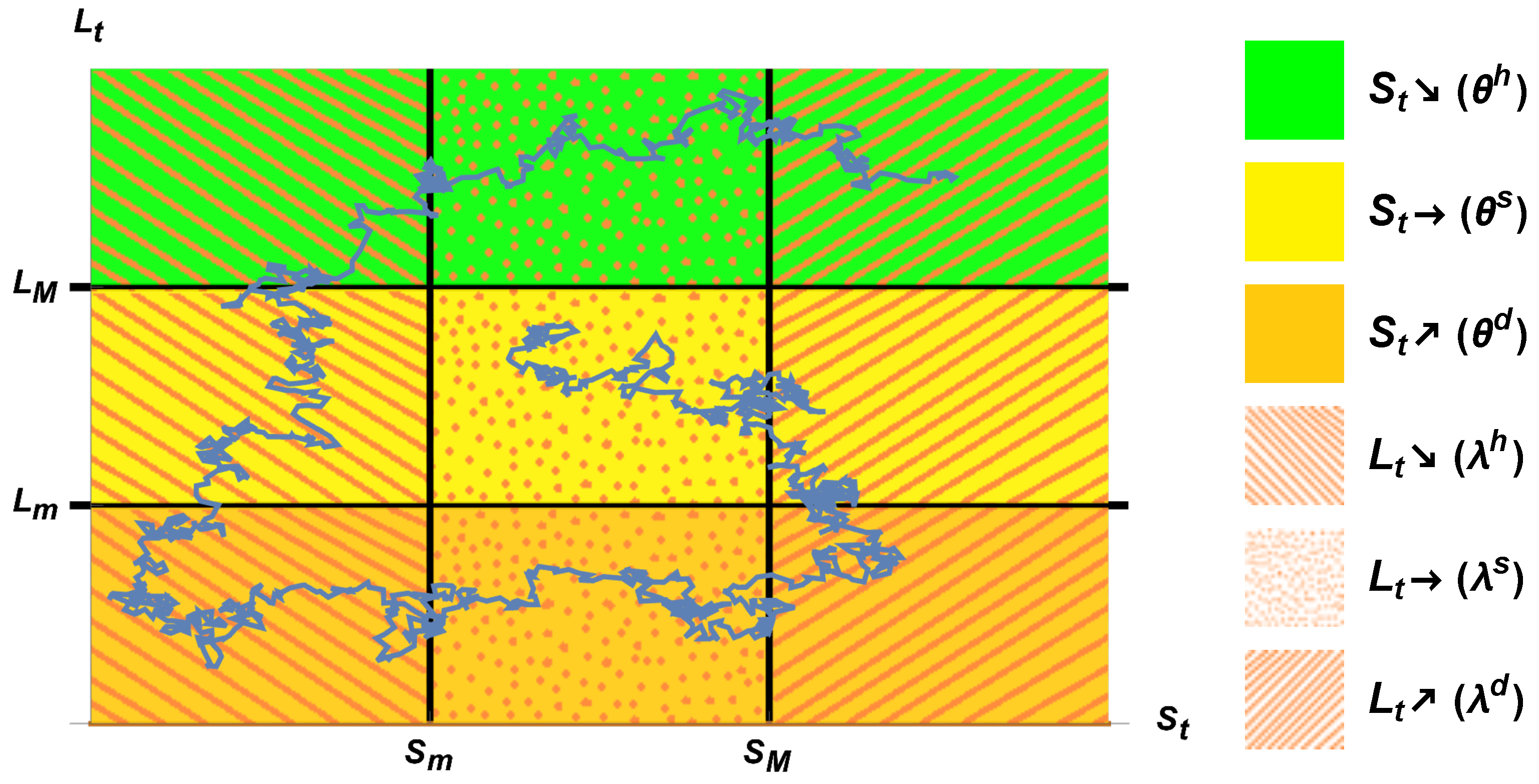
Figure 2.
A global view of a joint trajectory crossing one of their respective (double) thresholds at random times.
Figure 2.
A global view of a joint trajectory crossing one of their respective (double) thresholds at random times.

Figure 3.
A local view of a joint trajectory crossing one of their respective (double) thresholds at random times.
Figure 3.
A local view of a joint trajectory crossing one of their respective (double) thresholds at random times.

Figure 4.
Ford Motor Company’s volume of transactions and a trajectory of an EOU process.
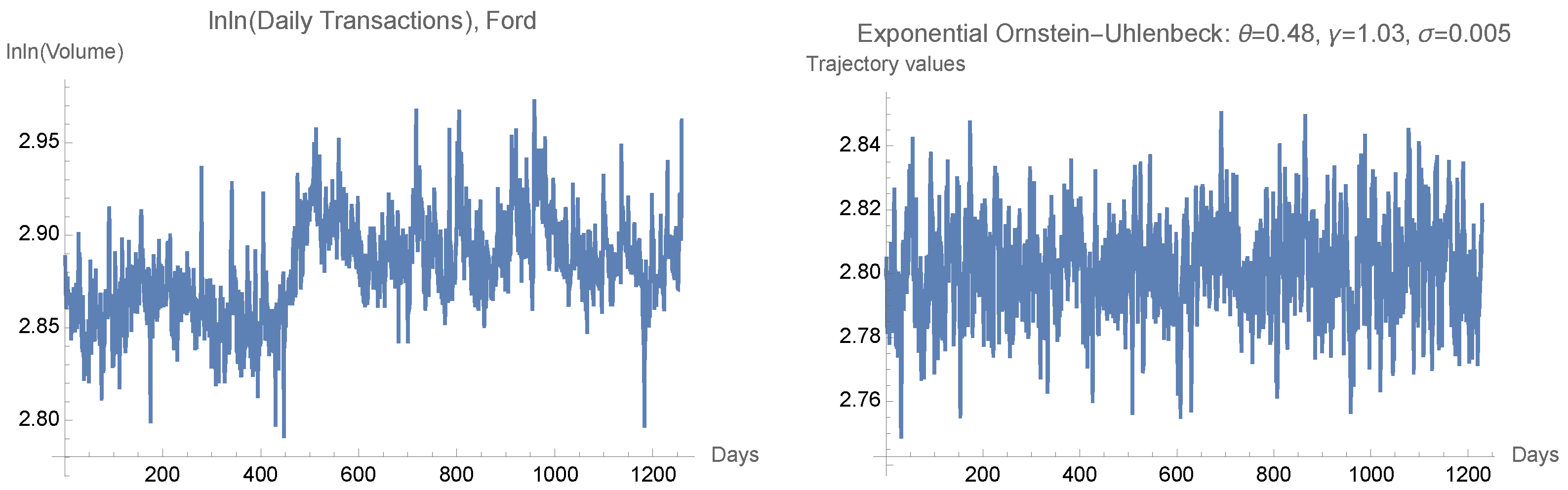
Figure 5.
On the left, Ford Motor Company price–volume of transactions and estimated thresholds values: Volume: 2.92666, 2.84673; Prices: 2.95864, 1.86765; On the right, schematic representation of the dynamic (Price–Volume) from the estimated parameters.
Figure 5.
On the left, Ford Motor Company price–volume of transactions and estimated thresholds values: Volume: 2.92666, 2.84673; Prices: 2.95864, 1.86765; On the right, schematic representation of the dynamic (Price–Volume) from the estimated parameters.

Table 1.
Some 16 scenarios of possible (Price,Volume) dynamics.
| Scenarios | I | II | III | IV | V | VI | VII | VIII |
| Liquidity on highest price subdomain | ↑ | ↓ | ↓ | ↓ | ↓ | ↓ | ↓ | ↓ |
| Liquidity on lowest price subdomain | ↓ | ↓ | ↓ | ↓ | ↓ | ↑ | ↑ | ↑ |
| Price on highest liquidity subdomain | ↓ | ↓ | ↓ | ↑ | ↑ | ↓ | ↓ | ↑ |
| Price on lowest liquidity subdomain | ↑ | ↓ | ↑ | ↓ | ↑ | ↓ | ↑ | ↓ |
| Scenarios | IX | X | XI | XII | XIII | XIV | XV | XVI |
| Liq. on highest price subdomain | ↓ | ↑ | ↑ | ↑ | ↑ | ↑ | ↑ | ↑ |
| Liq. on lowest price subdomain | ↑ | ↓ | ↓ | ↓ | ↑ | ↑ | ↑ | ↑ |
| Pri. on highest liquidity subdomain | ↑ | ↓ | ↑ | ↑ | ↓ | ↓ | ↑ | ↑ |
| Pri. on lowest liquidity subdomain | ↑ | ↓ | ↓ | ↑ | ↓ | ↑ | ↓ | ↑ |
Disclaimer/Publisher’s Note: The statements, opinions and data contained in all publications are solely those of the individual author(s) and contributor(s) and not of MDPI and/or the editor(s). MDPI and/or the editor(s) disclaim responsibility for any injury to people or property resulting from any ideas, methods, instructions or products referred to in the content. |
© 2023 by the authors. Licensee MDPI, Basel, Switzerland. This article is an open access article distributed under the terms and conditions of the Creative Commons Attribution (CC BY) license (https://creativecommons.org/licenses/by/4.0/).
Share and Cite
MDPI and ACS Style
Esquível, M.L.; Krasii, N.P.; Mota, P.P.; Shamraeva, V.V. Coupled Price–Volume Equity Models with Auto-Induced Regime Switching. Risks 2023, 11, 203. https://doi.org/10.3390/risks11110203
AMA Style
Esquível ML, Krasii NP, Mota PP, Shamraeva VV. Coupled Price–Volume Equity Models with Auto-Induced Regime Switching. Risks. 2023; 11(11):203. https://doi.org/10.3390/risks11110203
Chicago/Turabian StyleEsquível, Manuel L., Nadezhda P. Krasii, Pedro P. Mota, and Victoria V. Shamraeva. 2023. "Coupled Price–Volume Equity Models with Auto-Induced Regime Switching" Risks 11, no. 11: 203. https://doi.org/10.3390/risks11110203
Note that from the first issue of 2016, this journal uses article numbers instead of page numbers. See further details here.