Abstract
Green bonds are an increasingly important area not only in the financing of investments important to the environment, but recently also as an object of investment. From the investors point of view, the key aspect still remains the efficiency of the investment and its profitability. The subject of this research is to evaluate changes in the efficiency of green bonds issued in the selected CEE countries (Poland, Slovakia, Czech Republic, and Hungary), in the short and long term. Poland is the largest issuer of green bonds in this group, followed by the Czech Republic, Hungary, and Slovakia. Individual green bonds in these group of countries are characterized by varying levels of green bond yields, duration of the investment, issue size and counterparty risk. These factors greatly hinder their comparability, especially in terms of investment efficiency. This manuscript fits into this area, as the main purpose of the manuscript is to show similarities in the yields of green bonds issued in Poland and green bonds issued in CEE countries. The hypothesis that will be tested is that changes in the effectiveness of green bonds issued in Poland are strongly correlated with changes in the effectiveness of green bonds issued in CEE countries. The results of the research positively verified the hypothesis, and the objectives of the research were achieved. It was shown that green bonds issued in the Czech Republic and Slovakia demonstrate a high similarity in terms of effectiveness to green bonds issued in Poland. At the same time, the results confirmed that of all the bonds analysed, the one bond issued by the Hungarian government is the least related to green bonds issued in Poland in terms of effectiveness for investors. The study used multiresolution analysis and Dynamic Time Warping. The Dynamic Time Warping algorithm measures the similarity between two sequences that can change over time. The analysis was carried out over a wide temporal cross-section, analysing the similarity between the effectiveness in both the short and long term.
1. Introduction
The progressive degradation of the natural environment, causing far-reaching and irreversible climate change, requires decisive action to change the existing mechanisms by which economies around the world function. The cause of adverse environmental changes is primarily an environmental social and economic imbalance, which can be addressed through global ecological transformation and through the implementation of global sustainable development policies. The concept of sustainable development mainly refers to the efficient use of natural resources while protecting the environment. A key aspect of sustainable development is therefore to ensure economic growth while maintaining environmental sustainability (Robinson 2004).
The first attempt to introduce the idea of sustainable development was made in the 1980s, and since then the concept has been continuously updated. By the year 2000, the United Nations (UN) had implemented the Millennium Project, in which it set out eight Millennium Development Goals. However, 12 years later, in June 2012, the UN began the process of setting new development goals. Ultimately, this process ended with the adoption in September 2015 of a global action program based on the concept of sustainable development, presented in the document Transforming our world: the 2030 Agenda for Sustainable Development (United Nations 2015). The Agenda contains 17 Sustainable Development Goals (and 169 related tasks), the role of which is to integrate activities in three dimensions of sustainable development: economic, social, and environmental (Ministerstwo Rozwoju i Technologii 2019). Additional environmental protection activity has also been undertaken in Europe. In December 2019, the European Commission presented a set of policy initiatives called the European Green Deal. The overarching goal of the Green Deal is to achieve climate neutrality in Europe by 2050.
The financing of environmentally oriented projects, so-called ‘green investments’, plays an important role in maintaining climate balance and achieving climate neutrality. By 2030, it is estimated that Europe will need an additional investment of EUR 480 billion per year to achieve environmental goals, including as much as EUR 350 billion per year to reduce greenhouse gas (GHG) emissions (Kotecki 2021). The widespread demand for green investments in the global economy has become a central issue and challenge for financial markets. As a result, recent years have seen a marked increase in green activity by financial institutions and a rapid development of the market for environmentally oriented financial instruments.
Green bonds are becoming a key instrument in the financing of green investments. Green bonds are fixed-income debt securities, similar in design to classic bonds. The characteristic that distinguishes green bonds from classic bonds is the purpose of the issue. The purpose of issuing green bonds is always oriented towards financing or refinancing activities aimed at environmental protection (Hadaś-Dyduch et al. 2022; Gemra 2021; Ehlers and Packer 2017; OECD 2015), et al. Green bonds thus represent a commitment by the issuer to use the money raised through their issuance exclusively for environmental purposes (Hadaś-Dyduch et al. 2022). The issue of green bonds was initiated by the European Investment Bank in 2007–2008. Since then, the green bond market has been growing steadily, and as the market grows, different types of green bonds are emerging (Figure 1).
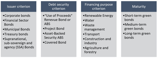
Figure 1.
Classification of green bonds. Source: Own study based on (OECD 2015; Doran and Tanner 2019; MSRB 2018).
The subject of the research is the effectiveness of green bonds issued in Poland and selected countries of Central and Eastern Europe in the short and long term. This formulation of the subject of the research is justified by both theoretical and practical considerations. The main rationale for undertaking research on the effectiveness of green bonds in CEE countries is the poor state of knowledge in this area. There are only a few studies in the reference literature focusing on the green bond market in the European Union (Dan and Tiron-Tudor 2021; Frydrych 2021), globally (Laskowska 2017) and in individual CEE countries (Gemra 2021; Sági 2020). However, there is no holistic approach to the green bond market in the CEE countries, nor studies comprehensively showing the relationships between the green bond markets in the CEE countries, especially in terms of their efficiency. The research gap identified on the basis the source literature justifies the need to undertake research in this area. The issue of the effectiveness of green bonds in CEE countries is important both for issuers, investors, and the entire economy.
Previous studies have reported that since 2016, i.e., from the creation of the green bond market in the CEE countries, both the number of issues and the value of funds raised have varied. The number of green bond issues in the analysed countries varied: nine issues were carried out in Poland, eight issues were carried out in Hungary, seven issues were carried out in the Czech Republic, and only one green bond issue was carried out in Slovakia. (Hadaś-Dyduch et al. 2022). As a result, the main objective of the manuscript is to identify similarities in terms of the effectiveness of green bonds issued in Poland and other selected Central and Eastern European countries—both in the long and short term. The implementation of the research goal required the calculation of an effectiveness index for each green bond, followed by application of the author’s algorithm based on multiresolution analysis and an algorithm based on Dynamic Time Warping. The Dynamic Time Warping algorithm measures the similarity between two sequences that can change over time. The analysis was carried out over a wide temporal cross-section, analysing the similarity between the effectiveness in both the short and long term.
This manuscript puts forward the following hypothesis: changes in the effectiveness of green bonds issued in Poland are strongly correlated with changes in the effectiveness of green bonds issued in CEE countries.
2. Literature Review
As previously stated, green bonds are debt instruments which allocate the proceeds of emissions exclusively to the financing or refinancing of new or existing green projects. Projects usually cover a wide range of activities:
- Climate change adaptation;
- Environmental protection;
- Energy efficiency and renewable energy;
- Sustainable water and wastewater management;
- Reduction of air pollution;
- Biodiversity protection;
- Transport;
- Others.
The criteria for categorising projects as green can vary from sector to sector and from region to region (Karginova-Gubinova et al. 2020).
Green bonds are instruments that are used to reduce the supply and demand gap for financial resources related to the financing of broadly understood ecology. Ehlers and Pecker (Ehlers and Packer 2017) believe that there must be favourable market conditions for the developing green bond market, ensuring adequate profitability for both issuers and investors. Therefore, as emphasized by Deribew (2017), the issuance of green bonds should be based on a few key principles, as described below:
- Use of the proceeds of the issue—the issuer should declare the eligibility of the project financed through the bonds to the relevant green investment category, which should be supported by legal documentation; there should be clear environmental benefits associated with the project(s) financed through the issue of these bonds; green investment areas include, among others: biodiversity conservation, low-carbon transport energy efficiency and renewable energy, clean water, and sustainable waste management.
- Selection and evaluation process—the investment decision-making process should be well described by the issuer to determine the eligibility of investments using green bond proceeds; they should also document the eligibility of investments into a particular category of green projects.
- Proceeds management—funds raised through the issuance of green bonds should be disclosed and transferred to a subportfolio or confirmed by another formal internal process; investors should be informed by the issuer of the intended types of eligible instruments used in the implementation of the green project.
- Reporting—reports on the implementation of investments made with funds raised through the issuance of green bonds should be submitted by the issuer at least once a year, detailing where possible the environmental benefits through quantitative/qualitative indicators, e.g., reduction in greenhouse gas emissions, number of people provided with access to clean energy, or clean water projects (Deribew 2017).
The green bond market (mainly in the CEE countries) is still in its infancy, so it is worth noting the determinants of its development. The main determinant is the type of projects that are financed with green bonds, given that regulators around the world are developing their own criteria for financing using these instruments. Moreover, projects financed through this instrument require an appropriate use of resources, so a specific project must meet several conditions set out in the regulator’s guidelines (Bhutta et al. 2022).
Research often highlights the quality of information in relation to green bonds. Martin and Moser (2016) emphasise that investors prefer quality of information when making investment decisions, and positively view those bonds in which issuers provide detailed information on the use of funds and environmentally friendly projects in the long term. As a result, these instruments are perceived as a safe investment. Biddle et al. (2009) emphasise that the quality of information is essential in gaining the trust of bondholders. In contrast, Hafner et al. (2020) highlighted elements that inhibit the expansion of green investments (including green bonds). They pointed out that unintelligible green financing policies and misinformation are some of the many factors that act as impediments to green financing.
Flaherty et al. consider that immediate investments (for example in climate change mitigation) could be financed by issuing green bonds so that future generations who will benefit from these actions can repay the debt (Flaherty et al. 2017). Moreover, they point out that the intergenerational burden-sharing formula is one way to develop the green bond market, while the main macroeconomic drivers of long-maturity bonds (to which green bonds belong) are production, inflation rates, and interest rates. High inflation rates, for instance, significantly limit the issuance of these bonds. On the other hand, high interest rates encourage shorter bond durations. Reduced production and income are also associated with reduced issuance of long-maturity bonds.
The source literature also discusses the cost of green bonds capital. Various researchers claim that financing environmentally friendly and sustainable projects, helps reduce the capital cost. Their main case is that market participants positively perceive issuers involved in social projects that provide low-cost financing. In contrast, other researchers argue that the most important concern of the issuer is increasing returns to shareholders, and as green bonds are riskier than conventional bonds, investors demand higher returns on them (Bhutta et al. 2022).
Preclaw and Bakshi note several important issues related to the cost of green bonds (Preclaw and Bakshi 2015). The price of green bonds may reflect the growing demand for these instruments and, as a result, indicate an imbalance in supply and demand for green issues. In this situation, the spread differential may not continue indefinitely. If issuers perceive an opportunity for cheaper financing, they can be expected to lean towards the market; at the same time, lower future yields resulting from narrower spreads may reduce the inflow of funds for green investments. Moreover, green bonds should be traded with narrower spreads to reflect their externalities, such as mitigating climate risk by engaging in environmental projects. Narrower green bond spreads may simply reflect a preference on the part of investors, which may be the case if investors accumulate enough other benefits to compensate for the lower cash flow. These benefits may, for example, take the form of psychological benefits for investors, brand value, impact on regulators or other indirect benefits. Investors positively disposed towards green investments suggest that they want to receive risk-adjusted remuneration, which is the equivalent of conventional investments.
Caramichael and Rapp (2022) indicate that there are several direct and indirect benefits to issuers of green bonds, which potentially should encourage green investment. If an issuer chooses to issue green bonds, this can attract new investors interested in sustainable investments, thereby increasing demand for them. If the additional demand results in green bond yields being lower than those of conventional bonds, this difference in yield is called the green premium or ‘greenium’. However, it is important to note that even if green bond issuance offers greenium, green bond issuance may still be more expensive compared to conventional bonds. From an investor’s point of view, there are a few explanations why investors accept the lower green bonds yield compared to similar traditional bonds. The frequent explanation for green-premium (greenium) is that investors accept a lower return for an environmental benefit. Green bonds actually consist of a traditional bond that has the added value of financing green projects. Therefore, investors accept the lower yield of green bonds and are willing to pay a higher price for the bond. By optimising the compromise between environmental impact and returns, investors should apply demand pressures that will create ‘smart greenium’, rewarding credible green bonds with a high incremental impact and lower interest rates.
On the other hand, Zerbib (2019) investigated factors associated with low green bond issuance costs, and found that the lower cost of green bond debt does not depend on the so-called issue greening, but it is result of other elements, i.e., reduced investor search for sustainable investments, risk management through intangible asset management, etc. Ehlers and Packer (2017) emphasize that a significant part of investors accept a lower spread and thus express their intention to pay a premium for green bonds, and that this should be evident in an increase in bond prices at issuance. At the same time, they argue that not all issuers can benefit from yield reduction when green bonds are issued. Partridge and Medda (2020) point out that green bonds must be competitive in all respects to prove attractive to investors who are subject to a fiduciary duty, i.e., they are required to put yields ahead of all other investments. They argue that green assets can deliver returns that are as good or better than their conventional counterparts, in which case investors may become interested in them and help invest in sustainability at the same time. Moreover, notwithstanding the clear greenium, issuers still seem to like issuing green bonds for various reasons, e.g., raising their sustainability profile, and are not as focused on generating greenium as some investors. Issuers also seem to enjoy attracting a new investor base rather than focusing on pricing, as long as the pricing is competitive with the overall market. Nevertheless, greenium is still key to the green bond market growth, as it is primary market prices that ultimately affect the cost of capital for the issuer, not secondary market prices. Larcker and Watts (2020) conclude that in actual market conditions, investors are categorically unwilling to give up environmentally friendly assets. When the risks and returns are fixed and known to investors ex ante, investors view green and non-green securities from the same issuer as almost exact substitutes. Thus, the greenium is essentially zero. Kapraun et al. (2021) find that all things being equal, there is no difference in yields for green bond issues. However, the existence and significance of the green premium varies considerably depending on the currency and type of issuer. It is high and significant for bonds issued by public entities, like governments, supranational organisations, or for bonds denominated in EUR.
In addition to direct environmental benefits, green bonds also provide indirect benefits, for example by pointing to the issuer’s environmental experience, providing a marketing advantage, potentially lowering the issuer’s capital cost by engaging new investors, or improving business activity performance by acquiring new customers. This intermediate result is called a green halo (Caramichael and Rapp 2022). Flammer (2021) pointed out that investors react positively to the predictor of a green bond issue, with the reaction being stronger for first-time issuers and third-party certified green bonds. Issuers boost their post-issuance environmental results (i.e., environmental ratings are higher and CO2 emissions are lower) and attract a larger group of long-term and ecological investors. Tang and Zhang (2020) find that the issuance of green bonds has a positive impact on stock prices, but at the same time they do not find a significant premium for green bonds. This situation suggesting that the stock profits associated with green bond announcements are not fully driven by the lower cost of debt. They also show that after the issuance of green bonds, domestic institutional ownership increases. Moreover, the stock liquidity after the issuance of green bonds is significantly better.
Wang et al. (2020) examined the green bonds premium variables. They showed that green bond issuer characteristics help to produce a higher premium. Green corporate bond price growth is most evident in new issues with high levels of corporate social responsibility. It is also higher for corporate bond issues with a lower concentration of ownership and in the hands of long-term institutional investors. They also note the positive outlook for higher stock returns on new green bond issues, which is consistent with the theory of stakeholder value maximization, according to which corporate involvement in sustainable financing practices increases long-term corporate value and is therefore preferred by shareholders.
Agliardi and Agliardi on the other hand, discussed the volatility of green bonds from the investors’ point of view (Agliardi and Agliardi 2019). They pointed out that as investors become more knowledgeable about the Sustainable Development Goals, green bonds demand increases. They also show the influence of asset volatility that results in greenium for green bonds issuers (Chung et al. 2019). Chung et al. also presented the importance of volatility in bond pricing. They concluded that higher expected returns are generated by bonds with more specific risk. The benefits of diversification can be obtained by issuing different types of bonds in the market.
When discussing the issue of the green bond market, attention should be paid to its efficiency. The efficient market hypothesis was formulated by E. Fama (Karginova-Gubinova et al. 2020). According to this hypothesis, available information entirely determines the prices of financial assets. As a result, an investor can achieve a satisfactory rate of return only if he accepts greater risk taking into account market efficiency. E. Fama distinguished the following forms of market efficiency:
- Weak—all information reflected in past price movements is contained in current prices;
- Moderate—takes into account both past price dynamics and all price information that is publicly available;
- Strong—contains both all publicly available information and confidential information.
Currently, it is believed that all information is contained in the transaction prices of financial instruments. This is due to the large number of players involved in analysing and monitoring all data affecting the price of securities. It is estimated that their number (analysts and investors) is much higher than the number of financial assets traded. At the same time, due to the varying costs of access to data for different market participants at different times negatively verifies the efficient market hypothesis. In addition, it is observed that the rationality of investor behaviour is not confirmed in market prices, because investors may succumb to overconfidence, herd instinct or may draw wrong conclusions about losses or profits, and besides, they may succumb to calendar effects, which are characterized by abnormal changes in the profitability of securities specific to a certain time, day of the week, month, etc. (Karginova-Gubinova et al. 2020). From the perspective of green bond effectiveness, Bachelet et al. found that the higher yield of green bonds is influenced by higher liquidity, and at the same time green bonds show lower volatility compared to their counterparts (Bachelet et al. 2019). They also showed differences between institutional and private issues of green bonds. Institutional green bonds have a negative premium but higher liquidity. Private green bonds, on the other hand, are characterized by a positive premium but at the same time significantly lower liquidity compared to their counterparts. In contrast, in the case of green bonds from private certified and uncertified issuers, the positive premium was found to be very high for the latter. Green bonds may have a negative premium and may be issued taking into account:
- Discount;
- Investors’ willingness to pay for environmental sustainability;
- Less exposure to risk.
The premium imposes the need to maintain a good reputation of (institutional) issuers or ecological verification in order to reduce information asymmetry and provide investors with a guarantee against bonds greenwashing. Chiesa and Barua argue that the volume of green bond issuance is positively correlated with the financial condition of the issuer and its credit rating, with the coupon rate and the availability of collateral, and with the sector in which the issuer operates. (Chiesa and Barua 2019). Moreover, euro-denominated issues in emerging markets are much larger. Arguably, these features make bonds more reliable, safer, and generate returns for investors, making it easier to issue larger sizes due to greater investor demand. Karginova-Gubinova et al. believe that the efficient operation of the green bond market and appropriately economically justified quotes will effectively raise financing for green projects (Karginova-Gubinova et al. 2020). If financial abuses and stock market bubbles appear on the market, the amounts obtained from the issuance of green bonds will be insufficient due to the decreasing number of investors. The authors proved that the market of green bonds is currently not efficient, even in its weak form. This is in line with conclusions regarding calendar effects, which are not typical for green bonds. Therefore, in order to increase the efficiency of the green bond market, the supply of and demand for green bonds, and thus the development of the green economy, it is necessary to increase the rationality of potential investors in their analysis of information about green bonds (strong knowledge of the clean economy, resource-saving technologies, etc.), improve market models (high-quality work of financial analysts by increasing their number and thus competition; special education), reduce transaction costs and increase the availability of information (distribution of reports on the green bond market, the dynamics of their indices, etc.). Moreover, the standardization of the terms used and an increase in the number of investors, especially qualified institutional investors, will strengthen confidence in the market and influence trading trends, which will contribute to the efficiency of the green bond market.
3. Materials and Methods
3.1. Green Bond Issuance in Poland and other Selected CEE Countries
The first green bond issuance in selected CEE countries took place in 2016 in Poland, and in subsequent years also in the other countries surveyed. However, the countries differ in terms of:
- The numbers of green bond issues;
- The currency of green bond issues;
- The values of green bond issues (Poland ($5893.81 million), Czech Republic ($5582.61 million), Hungary ($3320.73 million) and Slovakia’s only to USD 361.38 million) (Environmental Finance Data 2022).
- By the sector:
- ○
- The state sectors were dominated in Poland and Hungary;
- ○
- The private sectors were dominated in Czech Republic and Slovakia.
In Poland, green bond issuance took place in both the private and public sectors. The main issuers of green bonds in Poland were two financial sector entities (mBank and PKO Bank Polski S.A.) and two non-financial companies (PKN Orlen and Cyfrowy Polsat S.A.). One of the issuers of the financial sector is mBank (the first fully online bank in Poland), which focuses on implementing innovations in online and mobile banking. Meanwhile, the second bank issuing green bonds in Poland was Bank PKO BP, whose activities have for many years been oriented towards the idea of sustainable development, and are in line with the European Green Deal programme. In addition to the financial sector, the non-financial sector was also an issuer of green bonds in Poland. The main issuer of green bonds in this sector was PKN Orlen. PKN Orlen is an energy company that focuses primarily on renewable energy and modern petrochemistry, as well as on searching for innovations in the field of new mobility, hydrogen energy and recycling. Cyfrowy Polsat’s activities, on the other hand, focus primarily on the provision of integrated media and telecommunications services, such as television services, telephone services, data services, and access to broadband internet. A detailed summary of private sector emissions in Poland is presented in Table 1.

Table 1.
Green bond issue in Poland (private sector).
In addition to the private sector, green bond issuance in Poland was carried out by the government. The Polish government carried out 4 green bond issues, denominated in EUR (Table 2).
Table 2.
Government green bond issue in Poland.
The Czech Republic was the second country among the CEE countries in terms of the value of green bonds issued. In the Czech Republic, the issuer of green bonds was exclusively the private sector. The nonfinancial sector accounted for a significant portion of the issuance ($4989.05 million), while the financial sector comprised issues worth only $593.56 million. The main issuer of green bonds in the Czech Republic during the period under review was CTP Group N.V. covering the logistics and industrial real estate sector in Central and Eastern Europe. The main evidence of the Company’s focus on sustainability is its BREEAM (Building Research Establishment Environmental Assessment Method) certificate, which confirms the implementation of the concept of sustainable development in infrastructure and buildings. The company has been raising capital through the issue of green bonds for three years. Another green bonds issuer in the Czech Republic was a bank belonging to the Erste Group-Ceska Sporitelna AS. The bank’s activities are oriented towards the idea of sustainable development, as evidenced by the constant adaptation of the bank’s business activities to protection of the environment. To date, Bank Ceska Sporitelna AS has carried out only one green bond issue (Table 3).
Table 3.
Green bond issue in Czech Republic.
Hungary was the third country in terms of green bond issuance among the selected CEE countries. The issuance of Hungarian green bonds covered the non-financial and financial public sectors and the private sector. To date, the Hungarian government has carried out six green bond issues, denominated in different currencies: HUF, EUR, USD, JPY, and Chinese Yuan (RMB). However, due to the availability of statistical data, only two issues are subject to empirical analysis (Table 4).
Table 4.
Green bond issue in Hungary.
The CEE group also includes Slovakia, which has the smallest number of green bond issues compared to the group as a whole. There was only one issue in Slovakia, which was carried out by Tatra Banka, a leader in financial innovation in the Slovak market (Table 5).
Table 5.
Green bond issue in Slovakia.
3.2. Method
In our research, we take into account the entire maturity of the tested green bonds. A modified proprietary WDTW algorithm was used in the research. This algorithm is based on wavelet analysis and dynamic time warping. The DTW algorithm in this model was implemented to measure the degree of similarity of changes in the examined time series between green bonds issued in selected countries of Central and Eastern Europe. In addition, the wavelet in the proprietary WDTW model is used to perform a wavelet decomposition of the analysed time series and to examine their similarity in specific time trends.
In the first step of the algorithm, based on detailed information about the green bonds analysed (issue prospectus, stock exchange quotations, etc.), the current rate of return on the bond for its holder was calculated. The measurement—the current rate of return on the bonds—is calculated as the quotient of: the market price of the bond by the closing price of the session and the amount of annual coupon payments specified in the bond issue prospectus. For each bond, we obtain a one-dimensional series that has a certain number of observations.
The series included in the study are not equinumerous, nor are they multiples of two. The size of individual series representing the current rate of return on bonds is presented Table 6:
Table 6.
Individual series representing the current rate of return on green bonds.
In the next step, we extend the time series. We expand the series using appropriate methods so that the number of each series is a multiple of 2. Various methods of extending finite series are given in the literature, e.g., zero-padding, assumption of periodicity of the signal, mirror reflection at the end of the signal, and similar methods. Each method has its advantages and disadvantages. The degree of the advantages and disadvantages of the methods of extending the series depends on many factors, one of which is the specificity of the examined series.
The next key step in the algorithm is wavelet decomposition. Series presenting the current rate of yield on bonds are subjected to wavelet decomposition at different levels of resolution. Based on the discrete wavelet transform algorithms, we determine the coefficients for short-term and long-term dependencies in the context of the analysed series. At this stage, we obtain details and approximations. An example wavelet decomposition is shown in Figure 2 below.
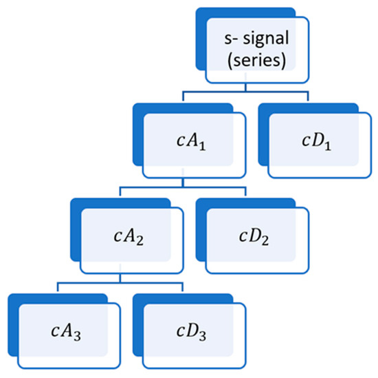
Figure 2.
Wavelet decomposition of the signal s analysed at level 3.
The last step of the algorithm is to determine the similarity between the series, i.e., to determine to what extent the analysed series have similar changes. To achieve this goal, we use dynamic wavelet transform (proprietary name), i.e., the distance (describing the degree of similarity) between the appropriate coefficients of the wavelet transform of the examined time series at specific levels of decomposition.
The maximum number of steps of the algorithm depends on the length of the examined series. In the case of series of different lengths, the number of maximum steps depends on the number of elements of the shortest series included in the study.
3.3. Theoretical Background to the Method
3.3.1. Dynamic Time Warping (DTW)
The Dynamic Time Warping algorithm is typically used to match two time series that differ in distance, length, time, and run rate. All linearized data can be examined by the DTW algorithm and distances can be measured using Euclidean distance or other distance measurement methods (Rabiner et al. 1978; Myers and Rabiner 1981). The procedure for the DTW algorithm is as follows:
- Introduction to the time series algorithm:
- X—of length N
- Y—of length M.
- Development of a grid of dimensions N × M, where in each of its fields is calculated the distance between samples of signals with numbers N and M, where N = 1, 2, …, N and M = 1, 2, …, M.
- Determination of the path W—the path W connects points (1, 1) and (N, M) so that the cost of transition between these points is as low as possible and must meet the following conditions:
- Boundary—which the first points of the X and Y waveforms and the last points of these waveforms coincide, which ensures that the entire time series waveforms will be matched to each other,
- Monotonicity—which guarantees correct synchronization of time courses and none of the time series will go back in time during matching,
- Step length—which ensures that no element of the X and Y waveforms will be missed, because subsequent points on the matching path cannot be too far away on the matched waveforms.
Each successive point on the W path must be indicated so that it is adjacent to the previous point, and the N and M indices cannot be reduced. The generated path is called the optimal alignment path.
Determining the distance between two points requires matching two signals, which are calculated as the sum of the values of all fields through which the path passes—more on how the algorithm works is presented in (Hadaś-Dyduch 2019b).
3.3.2. Wavelet Analysis
Wavelets are mathematical tools that, in an improved way (compared to the windowed Fourier method), make it possible to analyse the properties of signals in the neighbourhood of selected time moments, (more in (Hadaś-Dyduch 2019a, 2019b; Daubechies 1990; Rakowski 2003), among others). Fundamental features of the wavelet:
- Absence of a constant component;
- Occurrence of oscillations;
- In a finite interval the wavelet should be different from zero and outside this interval it should fade very fast, e.g., exponentially.
The wavelet transform, Wf(t,s), is the scalar product of the signal f(t) and the scaled and shifted wavelet:
where:
As can be seen from the above formulas, the wavelet transform of a function of one variable, is a function of time and scale. Since the calculation of the wavelet transform is labour-intensive and expensive, the following formulas are used, allowing the wavelet transform to be reversible (Rakowski 2003):
where a > 0, b > 0 are time-scale plane discretization parameters.
- Digital filters are used to calculate the discrete wavelet representation of the signal:
- Low-pass h;
- High-pass g.
In the case of transformations, only the low-pass filter h is sufficient, being the base for the high-pass filter g. The wavelet is not directly used in discrete wavelet transforms, but its properties determine the values of the set of numerical coefficients that constitute the wavelet representation of the signal (Figure 3). The choice of wavelet determines the choice of associated digital filters appearing in the transformation formulas (Rakowski 2003).
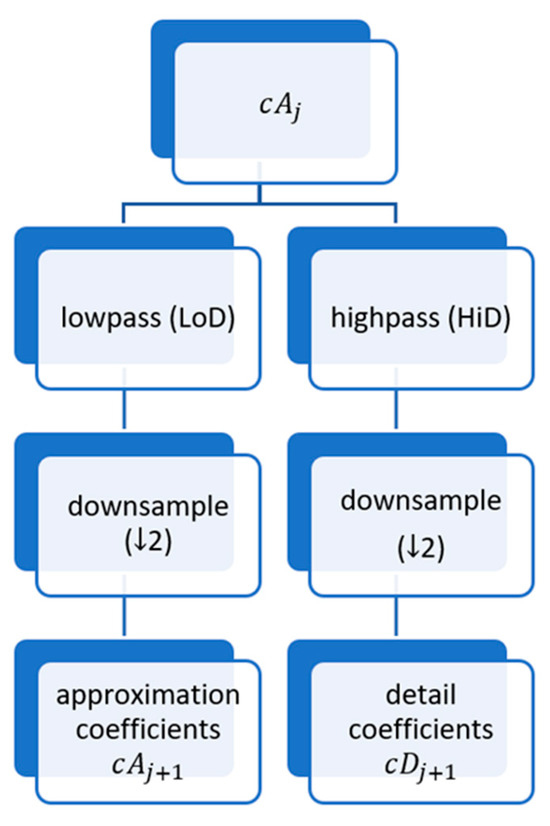
Figure 3.
One-Dimensional DTW.
There are many types of wavelets. Each wavelet has its advantages and disadvantages. Details in this regard are described, among others, in (Hadaś-Dyduch 2019b). One interesting wavelet is the Daubechies wavelet. This is an example of a compact wavelet. Details about this family of wavelets are described, e.g., in (Hadaś-Dyduch 2019a, 2019b; Daubechies 1990, 1992).
4. Results
The study included green bonds issued in the selected CEE countries. The study covered one bond issued in Slovakia, nine bonds issued in the Czech Republic, two bonds issued in Hungary, and six bonds issued in Poland. Detailed parameters concerning the bonds have been described in the previous chapter. Making a brief assessment of bond quotations in statistical terms, the following conclusions can be drawn (Table 7):
Table 7.
Selected statistical measurements of green signage quotations in individual countries of the CEE group.
- The average price of the analysed bonds ranges from EUR 81.41 to EUR 119.35.
- On average, the results deviate from the mean value by +/−0.45 to +/−9.06. The smallest deviation is in the case of C6 bonds issued by the Czech Republic, and the highest in the case of P4 bonds issued by Poland.
- Asymmetry coefficient—in the simplest terms—is a measurement used to study the shape of the feature distribution. In the analysed sample, the quotations of all the analysed bonds are characterized by left-sided asymmetry, i.e., the majority of quotations are above the average quotation price. The smallest asymmetry was observed for the W1 bond, a bond issued by Hungary, and the largest for the P4 bond issued by Poland.
- Kurtosis, which is used to assess the extent to which all observations are close to the average value, has a positive value for all the analysed bonds except for the W1 bond, i.e., we are dealing with slender distributions. In the case of three bonds, i.e., C6, P4, P5 bonds, the kurtosis is greater than 3, which means that the distribution of quotations is more slender than normal, and it can be assumed that there are two independent normal subpopulations with similar average values and different variances.
- The smallest spread (range—the difference between the maximum and minimum value from our set of observations) in bond prices was for C6 bonds and amounted to EUR 2.48. The lowest price of this bond was EUR 98.99 and the highest was EUR 101.47. The largest difference between the maximum value of quotations and the minimum value was recorded for P5 bonds and amounted to EUR 109.06.
The volatility of all the analysed bonds is low (see Figure 4), below 8%. The smallest diversification of quotations was recorded for C6 bonds—0.44%, and the highest for W1 bonds—8.65%.
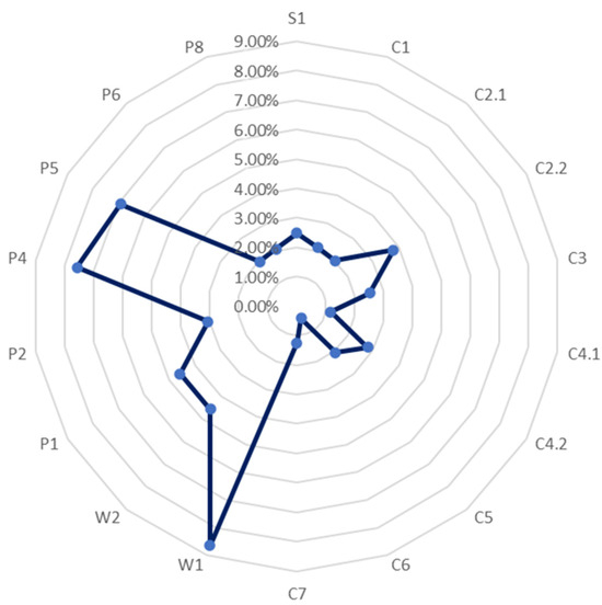
Figure 4.
Volatility coefficient for individual green bonds.
Quartile analysis provides a great deal of information (see Table 8). Data for the first, second, and third order quartiles are presented in the table below. We conclude, inter alia, that:
Table 8.
Quartile analysis.
- The largest quartile range is in the case of P4 bonds issued in Poland (coupon-3mWIBOR + 51 bps; issuer Bank PKO). It can be said that in the case of 25% of the quotations of P4 bonds, the price of the bonds was at or above EUR 119.06. On the other hand, in the case of 75% of the quotations of P4 bonds, the price of the bonds was at least EUR 119.07. Moreover, in the case of 50% of the P4 bonds, the price of the bonds was at or above EUR 122.82. In the case of 25% of the quotations of P4 bonds, the price of the bonds was at or above EUR 124.7. On the other hand, in the case of 75% of the quotations of P4 bonds, the price of the bonds was at least EUR 124.7.
- The smallest quartile range is for C6 bonds issued in the Czech Republic (CTP issuer). It can be said that in the case of 25% of the quotations of C6 bonds, the price of the bonds was at or above EUR 101. On the other hand, in the case of 75% of the quotations of C6 bonds, the price of the bonds was at least EUR 101. Moreover, for 50% of C6 bonds, the bond price was at or above EUR 101.1. In the case of 25% of the quotations of C6 bonds, the price of the bonds was at or above EUR 101.22. On the other hand, in the case of 75% of the quotations of C6 bonds, the price of the bonds was at least EUR 101.22.
Bond W1 has the largest quarter spread, and C6 the smallest (see Figure 5).
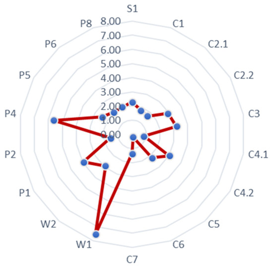
Figure 5.
Quarter range for individual green bonds. Source: Own calculations.
5. Detailed Results from the Empirical Study
The analysis of green bonds issued in Poland in the context of the similarity of changes with green bonds issued in other CEE countries was carried out in a spatial-temporal context. The analysis was conducted for various time trends, e.g., in a weekly, monthly, semi-annual, and annual trend.
Of course, in the first step, based on detailed information about the analysed green bonds (issue prospectus, stock exchange quotations, etc.), the current rate of return on the bond for its holder was calculated. The measurement—the current rate of return on the bond for its holder—was calculated as the quotient of: the market price of the bond by the closing price of the session and the amount of annual coupon payments specified in the bond issue prospectus. For each bond, a one-dimensional series with a specific number of observations was obtained. Then, the next steps of the WDTW algorithm were applied. The values obtained from the algorithm inform about the similarity. The smallest value is zero, which means 100% similarity between two time series. The higher the value of the WDTW measure, the smaller the similarity between the two series.
The conclusions of the study are described below in both spatial and temporal contexts.
5.1. Short-Term Trend
5.1.1. Trend 2–4 Days
Conclusion 1
Changes in the current rate of return of all green bonds issued in Poland in a two-day trend are very weakly related to changes in the current rate of return of W2 bonds issued in Hungary.
On a scale from 0 to 1, where the number one means no connection and the number zero means 100%, the following results were obtained based on the WDTW model:
- For P1 bonds—0.7416 (on a scale from 0 to 1);
- For P2 bonds—0.7931 (on a scale from 0 to 1);
- For P4 bonds—0.7979 (on a scale from 0 to 1);
- For P5 bonds—0.9973 (on a scale from 0 to 1);
- For P6 bonds—0.9973 (on a scale from 0 to 1);
- For P8 bonds—0.7847 (on a scale from 0 to 1).
As can be seen, all the results oscillate around 0.8, and WDTW (P5, S1) oscillates around 1, so the volatility of the current rate of return for a holder of bonds issued in Poland is not related in the 2–4-day trend to the volatility of the current rate of return for a W2 bond holder.
The W2 bond is a bond issued by the Hungarian government with a coupon of 1.75% (see Figure 6).

Figure 6.
The current rate of income (in %) for W2 green bonds issued in Hungary. Source: Own calculations.
However, it cannot be concluded that the current yields of all green bonds issued in Hungary do not have a similar volatility to the current yields of green bonds issued in Poland. This is because the W1 bond issued by the Hungarian government with a coupon of 4% shows a similar tendency of change to bonds issued in Poland (see Figure 7).
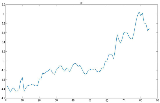
Figure 7.
The current rate of income (in %) for W1 green bonds issued in Hungary. Source: Own calculations.
On a scale from 0 to 1, where the number one means no connection and the number zero means 100%, the volatility of the W1 bonds is linked to the given bonds issued in Poland, and the following values of the WDTW index were obtained based on the WDTW model:
- For P1 bonds—0.1039 (on a scale from 0 to 1);
- For P2 bonds—0.1134 (on a scale from 0 to 1);
- For P4 bonds—0.1109 (on a scale from 0 to 1);
- For P5 bonds—0.4941 (on a scale from 0 to 1);
- For P6 bonds—0.1148 (on a scale from 0 to 1);
- For P8 bonds—0.0924 (on a scale from 0 to 1).
As can be seen, all the results oscillate around 0.1, except for WDTW (W1, P5), and therefore the volatility of the current rate of return for a holder of bonds issued in Poland is strongly related in the 2–4-day trend to the volatility of the current rate of return for a holder of W1 bonds.
Conclusion 2
Of all the analysed bonds, the W2 bond is the least related to changes in bonds issued in Poland in terms of effectiveness for its holder (see data in Figure 8 and Figure 9).
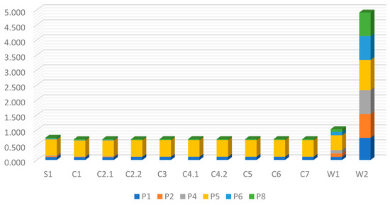
Figure 8.
WDTW index for individual bonds using only the first level of wavelet decomposition in the WDTW algorithm. Percentage analysis in the context of the analysis of all analysed bonds. Source: Own calculations.
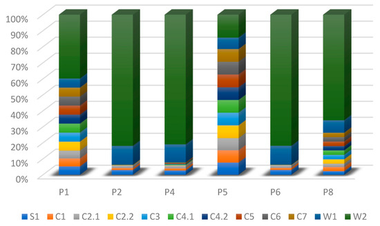
Figure 9.
WDTW index for individual bonds using only the first level of wavelet decomposition in the WDTW algorithm. Percentage analysis in the context of P1, P2, P4, P5 P6, and P8 bonds. Source: Own calculations.
Conclusion 3
Changes in the current rate of return of all green bonds issued in Poland in the 2–4-day trend are very strongly related to changes in the current rate of return of bonds issued in the Czech Republic. The exception is the P5 bond, where we only see a moderate link between the volatility of P5 bonds and bonds issued in the Czech Republic (see Table 9).
Table 9.
Values of the proprietary WDTW index for the indicated bonds, using only the first level of resolution in the algorithm.
The greatest dependence of bonds issued in the Czech Republic is with the bonds P2, P4, and P6. The smallest with the P5 bond.
Conclusion 4
All the green bonds issued in Poland (except P5 bonds) are in the 2–4-day trend and are very strongly related to changes in the current yield rate of green bonds issued in Slovakia. In the case of P5 bonds, we can talk about a moderate relationship between the volatility of the current rate of return of P5 bonds and S1 bonds (see Figure 10).
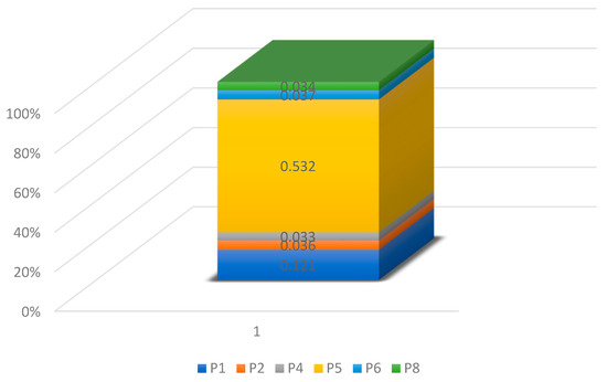
Figure 10.
Values of the proprietary WDTW index between the S1 bond and the P1, P2, P4, P5, P6, and P8 bonds, using only the first level of wavelet decomposition in the algorithm. Source: Own calculations.
The lowest correlation of current yields for a holder of a given bond, excluding the P5 bond, was observed between the P1 bond and the S1 bond. The P1 bond has a coupon of—3 month EURIBOR + 1.25% and the S1 bond has a coupon of—0.5% (see Figure 11 for the development of current yields for a holder of the S1 bond and the P1 bond).
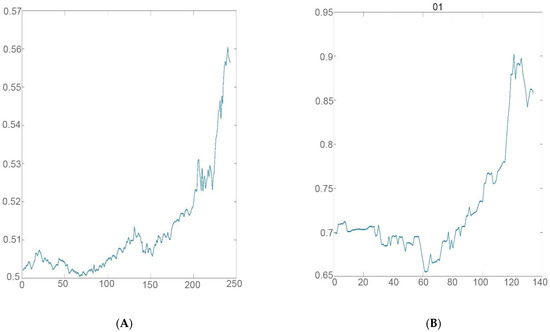
Figure 11.
The current rate of income (in %) for green bonds issued in Poland and Slovakia. (A) The current rate of income (in %) for S1 green bonds issued in Slovakia. (B) The current rate of income (in %) for P1 green bonds issued in Poland. Source: Own calculations.
Conclusion 5
In the 2–4-day trend, the current rate of return for a holder of the P5 bond shows volatility related only to the W2 bond. In the case of the other bonds, it shows a connection at a moderate level. The P5 bond is most closely related to the W1 bond (see Figure 12).
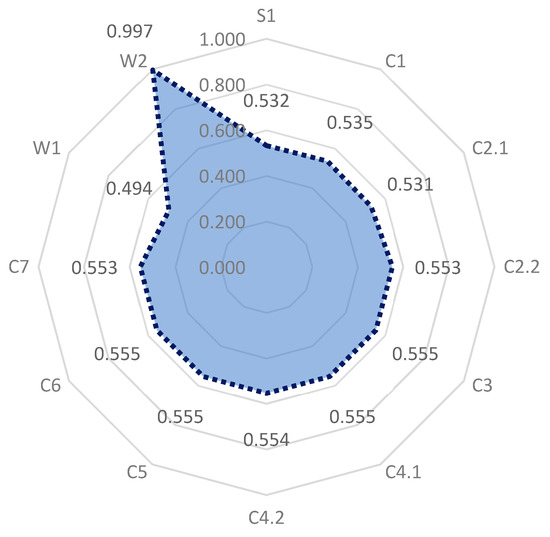
Figure 12.
Values of the proprietary WDTW index between the P5 bond and green bonds issued by the Czech Republic, Hungary, and Slovakia, using only the first level of wavelet decomposition in the WDTW algorithm. Source: Own calculations.
Table 10.
Brief characteristics of the P5 green bond.
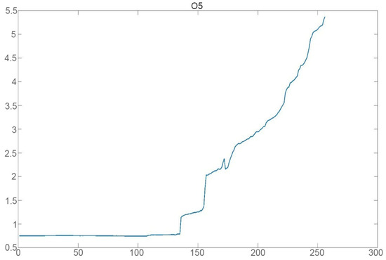
Figure 13.
The current rate of income (in %) for P5 green bonds issued in Poland.
5.1.2. Trend 4–8 Days
On the basis of the author’s model, appropriate calculations can also be made in order to assess the relationship between the tested bonds in the weekly trend. The conclusions are presented below.
Conclusion 1
Changes in the current rate of return of all green bonds issued in Poland are, in the weekly trend, very weakly related to changes in the current yield rate of W2 bonds issued in Hungary. On a scale from 0 to 1, where the number one means no connection and the number zero means 100%, the following results were obtained based on the WDTW model:
- For P1 bonds—0.8657 (on a scale from 0 to 1);
- For P2 bonds—0.9735 (on a scale from 0 to 1);
- For P4 bonds—0.9958 (on a scale from 0 to 1);
- For P5 bonds—0.9250 (on a scale from 0 to 1);
- For P6 bonds—0.9958 (on a scale from 0 to 1);
- For P8 bonds—0.9937 (on a scale from 0 to 1).
As can be seen, all results oscillate around the value of 1, so the volatility of the current rate of income for a holder of bonds issued in Poland is not related in the weekly trend to the volatility of the current rate of income for a holder of W2 bonds. It should be noted that the P5 bond, which is moderately related in the case of links with other bonds, shows a strong link in the case of W2 bonds. The opposite is true for W1 bonds (see Figure 14).

Figure 14.
Values of the proprietary WDTW index between bonds W1, W2 and bonds P1, P2, P4, P5, P6, and P8, using the second level of wavelet decomposition in the WDTW algorithm. Source: Own calculations.
On a scale from 0 to 1, where the number one means no connection and the number zero means 100%, the volatility of the W1 bonds is linked to the given bonds issued in Poland, and the following values of the WDTW index were obtained based on the WDTW model:
- For P1 bonds—0.1179 (on a scale from 0 to 1);
- For P2 bonds—0.1597 (on a scale from 0 to 1);
- For P4 bonds—0.1575 (on a scale from 0 to 1);
- For P5 bonds—0.5231 (on a scale from 0 to 1);
- For P6 bonds—0.1601 (on a scale from 0 to 1);
- For P8 bonds—0.1323 (on a scale from 0 to 1).
As can be seen, all the results except for WDTW (P5, W1) are less than 0.17, so the volatility of the current rate of return for a holder of bonds issued in Poland is strongly related in the weekly trend to the volatility of the current rate of return for a holder of W1 bonds.
Conclusion 2
Of all the analysed bonds in the weekly trend, the W2 bond is the least related to changes in bonds issued in Poland in terms of effectiveness for its holder (see data in Figure 15 and Figure 16).
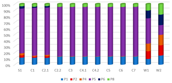
Figure 15.
WDTW index for individual bonds using the second level of wavelet decomposition in the WDTW algorithm. Percentage analysis in the context of the analysis of all analysed bonds. Source: Own calculations.
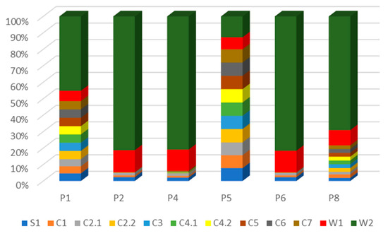
Figure 16.
WDTW index for individual bonds using the second level of wavelet decomposition in the WDTW algorithm. Percentage analysis in the context of P1, P2, P4, P5 P6, and P8 bonds. Source: Own calculations.
Conclusion 3
Changes in the current yield rate of all green bonds issued in Poland, with the exception of P5 bonds, are in the weekly trend very strongly related to changes in the current yield rate of bonds issued in the Czech Republic (see Figure 17).

Figure 17.
Treemap showing the strength of the relationship between the current rate of return for a holder of bonds issued in the Czech Republic and bonds issued in Poland in the weekly trend. (A) Treemap showing the strength of the relationship between the current rate of return for a holder of bonds issued in the Czech Republic with the P1 bond. (B) Treemap showing the strength of the relationship between the current rate of income for a holder of bonds issued in the Czech Republic with the P2 bond. (C) Treemap showing the strength of the relationship between the current rate of return for a holder of bonds issued in the Czech Republic with the P4 bond. (D) Treemap showing the strength of the relationship between the current rate of return for a holder of bonds issued in the Czech Republic with the P5 bond. (E) Treemap showing the strength of the relationship between the current rate of return for a holder of bonds issued in the Czech Republic with the P6 bond. (F) Treemap showing the strength of the relationship between the current rate of return for a holder of bonds issued in the Czech Republic with the P8 bond. Source: Own elaboration based on calculations in the Matlab program.
For all green bonds issued in the Czech Republic, the WDTW index showing the “scale” of the relationship between the current rate of return on bonds issued in Poland for their holder with other analysed bonds in the two-day trend is less than 0.1 (on a scale from 0 to 1). The exception is the P5 bond; here the volatility linkage is at the base level.
The greatest dependence is with bonds P2, P4, and P6. The smallest is with the P5 bond. Therefore, based on the results, it can be concluded that the energy policy of the Czech Republic is similar to the energy policy in Poland (see Figure 17).
Conclusion 4
Changes in the current yield rate of all green bonds issued in Poland are, in the weekly trend, strongly related to changes in the current yield rate of bonds issued in Slovakia (see Figure 18). Only in the case of P4 bonds is there a moderate link between the current rate of return on the P4 bond and the green S1 bond.
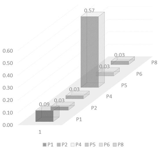
Figure 18.
WDTW index between S1 and P1, P2, P4, P5, P6, and P8 using second level wavelet decomposition in the WDTW algorithm. Source: Own calculations.
Conclusion 5
The analysis shows unequivocally that in the weekly trend, all bonds issued in Poland show volatility in the current rate of return for the holder that is strongly related to the volatility of bonds issued in Slovakia and the Czech Republic. The weakest relationship is with the P1 bond (see Figure 19). Only the P5 bond shows a moderate relationship.
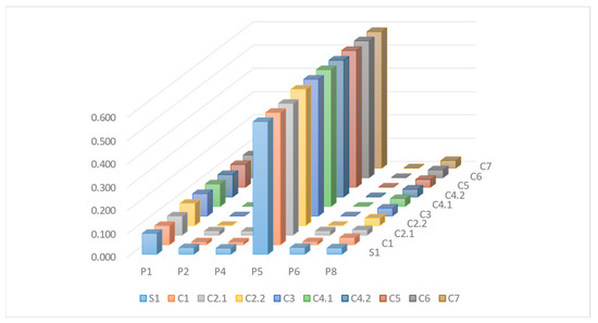
Figure 19.
WDTW ratio between bonds issued in the Czech Republic and Hungary and bonds issued in Poland using the second level of wavelet decomposition in the WDTW algorithm. Source: Own calculations.
5.2. Long-Term Trend
The data on which the empirical study were carried out are daily data. The rows are not equal. The maximum number of elements in the series is 256 observations. Therefore, various time periods were considered to constitute long-term trends in the article. Due to the fact that the P1 bond is described with a series of only 134 elements, it is not possible to consider the trend over a period longer than one or two months.
Conclusion 1
Analysis of bonds issued in Slovakia and those issued in Poland shows unequivocally that the volatility of the current rate of return for a holder of S1 bonds is linked to the volatility in the rate of return for a holder of the bonds P1, P2, P4, P6, and P8 in the long-term trend, monthly, two-monthly, and half-yearly.
As shown in Figure 20, there is a definite lack of connection between the volatility of the current rate of return for a holder of S1 and P5 bonds. It should be mentioned that the S1 bond is a bond issued by TATRA BANK, and the P5 bond by PKO BANK. The S1 bond has a coupon—0.5%, and the P5 bond—a 3-month WIBOR + 0.6%
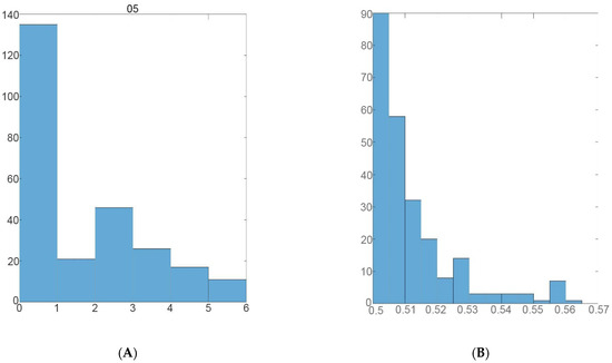
Figure 20.
Histograms presenting the current rate of income (in %) for individual analysed green bonds issued in Poland. Source: Own calculations. (A) Histogram presenting the current rate of income (in %) for P5 green bonds issued in Poland. (B) Histogram presenting the current rate of income (in %) for S1 green bonds issued in Slovakia. Source: Own calculations.
Statistical analysis of S1 and P5 bonds shows that:
- For S1 bonds:
- The current yield closes in the range of 0.5005 [%]–0.56 [%] (the difference is 0.06 [%]);
- The average value of this index is 0.512% with an error of 0.0008%;
- The index is characterized by low volatility (the coefficient of variation is 2.5%);
- The current yield index shows strong right-handed asymmetry (Figure 21) (asymmetry coefficient is 1.95[%], kurtosis is 3.46 [%]).
 Figure 21. WDTW index between a bond issued in Slovakia and bonds issued in Poland, using the WDTW algorithm in the trends 16–32 days, 32–64 days, 64–128 days. Source: Own calculations.
- For P5 bonds:
- The current yield closes in the range 0.744[%]–5.366[%] (the difference is 4.623 [%]);
- The average value of this rate is 1.806% with an error of 0.086%;
- The deviation from the mean is ±0.013% for S1, and ±1.382 for P5;
- However, the analysed index shows very high volatility for P5 bonds—the coefficient of variation is 76.5%;
- The current yield index shows centre-right asymmetry (Figure 21) (asymmetry coefficient is 1.0395 [%], kurtosis is—0.19 [%]).
Figure 22 indicates that:
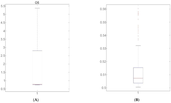
Figure 22.
Quantile analysis. The current rate of income (in %) for the analysed green bonds issued in Poland. (A) Quantile analysis. The current rate of income (in %) for P5 green bonds issued in Poland. (B) Quantile analysis. The current rate of income (in %) for S1 green bonds issued in Slovakia. Source: Own calculations.
- -
- For 50% of listings, the value of the current market rate of the green bond index is:
- For S1 bonds was not less than 0.50733%;
- For P5 bond was not less than 0.7535%.
- -
- For 25% of quotations, the value of the current market rate of green bonds is:
- For S1 bonds at most 0.50363%, (and for 75% listings at least 0.50363%);
- For P5 bonds at most 0.7335% (and at least 0.7535% in the case of 75% listings).
- -
- In the case of 75% of listings, the value of the current market rate of the green bond index is:
- For S1 bonds—at most 0.51586% (and for 25% of listings at least 0.51586%);
- For P5 bonds—at most 2.7956% (and for 25% of listings at least 2.7956%) (Figure 22).
Conclusion 2
Analysis of the bonds issued in the Czech Republic and the bonds issued in Poland clearly shows that the volatility of the current rate of income for a holder of these green bonds is related to the volatility of the current rate of income for a holder of P1, P2, P4, P6, and P8 bonds in the long-term trend, both monthly, and bi-monthly or half-yearly. There is no link only to the P5 bond.
As shown in the figure below, the WDTW ratio between bonds issued in the Czech Republic and the P1 bond is below 0.11. For the 16–32-day trend, the indicator ranges from 0.077 to 0.098 (on a scale of 0 to 1), for the 32–64-day trend, the indicator ranges from 0.083 to 0.108, and for the 64–128-day trend, the indicator values are between 0.063 and 0.078 (see Figure 23). All values are low, so the conclusion can be drawn that all green bonds issued in the Czech Republic have a current rate of return related to the volatility of the current rate of return of P1 bonds.
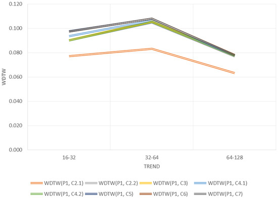
Figure 23.
WDTW between green bonds issued in the Czech Republic and P1 green bonds issued in Poland. Source: Own calculations.
The WDTW ratio between the bonds issued in the Czech Republic and the P2 bond is very low (see Table 11, Figure 24). For the 16–32-day trend, the indicator ranges from 0.0004 to 0.0206, for the 32–64-day trend, the indicator ranges from 0.0003 to 0.0166, and for the 64–128-day trend, the indicator values range from 0.0002 to 0.009. All values are very low, so it can be concluded that there is a very strong relationship between all green bonds issued in the Czech Republic and the P2 bond issued in Poland in terms of the yield of these bonds.
Table 11.
Values of the proprietary WDTW index between the current yield rate of bonds issued in the Czech Republic and the current yield rate of P2 bonds.
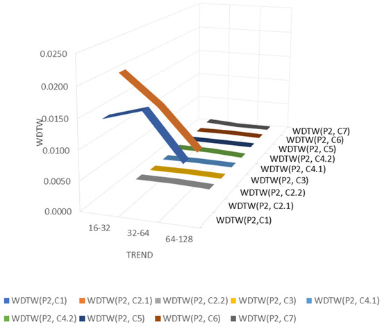
Figure 24.
WDTW between green bonds issued in the Czech Republic and P2 green bonds issued in Poland. Source: Own calculations.
The WDTW ratio between the bonds issued in the Czech Republic and the P4 bond is very low (see Table 12, Figure 25). For the 16–32-day trend, the indicator ranges from 0.005 to 0.021, for the 32–64-day trend, the indicator ranges from 0.002 to 0.018, and for the 64–128-day trend, the indicator values range from 0.003 to 0.011. All values are very low, although slightly higher than the WDTW ratio between the current yields of green bonds issued in the Czech Republic and the P2 bond. The ratio is lower than 0.022, so it can be concluded that there is a very strong link between all green bonds issued in the Czech Republic and the P4 bond issued in Poland in terms of the yield of these bonds.
Table 12.
Values of the proprietary WDTW index between the current yield rate of bonds issued in the Czech Republic and the current yield rate of P4 bonds.
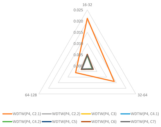
Figure 25.
WDTW between green bonds issued in the Czech Republic and P4 green bonds issued in Poland. Source: Own calculations.
The WDTW ratio, calculated for current bondholder yields between bonds issued in the Czech Republic and the P4 bond, assumes very high values (see Table 13, Figure 25). The values oscillate between 0.84 and 1 (on a scale from 0 to 1, where 1 means no similarity and 0 means complete similarity between the two series). For the 16–32-day trend, this indicator ranges from 0.968 to 1, for the 32–64-day trend, the indicator ranges from 0.91 to 0.926, and for the 64–128-day trend, the indicator values range from 0.833 to 0.844. All values are very high, so it can be concluded that there is no link between all green bonds issued in the Czech Republic and the P5 bond issued in Poland in terms of the yield of these bonds.
Table 13.
Values of the proprietary WDTW index between the current yield rate of bonds issued in the Czech Republic and the current yield rate of P5 bonds.
It should be noted that the value of the WDTW ratio for the current yield rate of bonds issued in the Czech Republic and the current yield rate of P5 bonds decreases as the time trend increases (see Figure 26). For example, for the relationship between C7 and P5, in the 16–32-day trend, WDTW (P5, C7) = 0.999, and in the 64–128-day trend, WDTW (P5, C7) = 0.844. Therefore, it can be concluded that the relationship between these bonds may occur over a long-term trend.
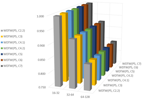
Figure 26.
WDTW between green bonds issued in the Czech Republic and P5 green bonds issued in Poland. Source: Own calculations.
The WDTW ratio between the current yields of bonds issued in the Czech Republic and the P6 bond has very low values, i.e., values below 0.02 (on a scale from 0 to 1). For the 16–32-day trend, the indicator ranges from 0 to 0.021, for the 32–64-day trend, the indicator ranges from 0 to 0.018, and for the 64–128-day trend, the indicator values range from 0 to 0.009. All values are very low (see Table 14, Figure 27) and therefore it can be concluded that there is a very strong relationship between the current yields of bonds issued in the Czech Republic and the P6 bond in terms of the yields of these bonds.
Table 14.
Values of the proprietary WDTW index between the current yield rate of bonds issued in the Czech Republic and the current yield rate of P6 bonds.
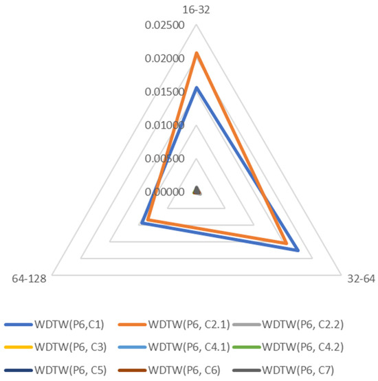
Figure 27.
WDTW between green bonds issued in the Czech Republic and P6 green bonds issued in Poland. Source: Own calculations.
Conclusion 3
The WDTW ratio between the current rate of return of the W1 bond issued in Hungary and the bonds issued in Poland ranges from 0.054 to 0.951 (on a scale from 0 to 1). The highest values of the indicator are for WDTW(W1, P5). The conclusion can be drawn that over the long-term trend there is no relationship in terms of yields between W1 and P5 bonds. A relationship can be established in the context of P1, P2, P4, P6, and P8 bonds, because their WDTW ratio with W1 bond is relatively low—below 0.2, on a scale from 0 to 1 (see Figure 28, Table 15).
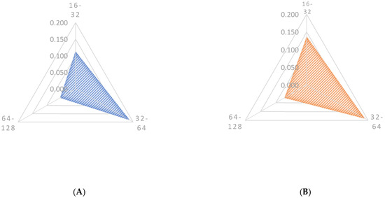
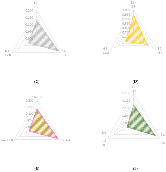
Figure 28.
WDTW between W1 green bonds issued in Hungary and green bonds issued in Poland. (A) WDTW(W1, P1). (B) WDTW(W1, P2). (C) WDTW(W1, P4). (D) WDTW(W1, P5). (E) WDTW(W1, P6). (F) WDTW(W1, P8). Source: Own calculations.
Table 15.
Values of the proprietary WDTW index between the current rate of return on W1 bonds and the current rate of return on bonds issued in Poland.
The WDTW ratio between the current rate of return of the W1 bond issued in Hungary and the bonds issued in Poland ranges from 0.28 to 1 (on a scale from 0 to 1). The highest values of the indicator are for WDTW (W2, P5). The conclusion can be drawn that over the long-term trend there is no relationship in terms of yield between the W2 bond and bonds issued in Poland (see Figure 29, Table 16).

Figure 29.
WDTW between W2 green bonds issued in Hungary and green bonds issued in Poland. Source: Own calculations.
Table 16.
Values of the proprietary WDTW index between the current rate of return on W2 bonds and the current rate of return on bonds issued in Poland.
6. Discussion and Conclusions
This study investigates the relationship between the yields of green bonds issued in Poland compared to the yields of green bonds issued in other CEE countries. The study was based on 20 green bond issues in CEE countries, including as many as 6 issues carried out in Poland. The aim of the article was to find an answer to the question whether the effectiveness of green bonds issued in Poland is related to the effectiveness of green bonds issued in other CEE countries in both the long and short term. A modified proprietary WDTW algorithm based on wavelet analysis and dynamic time transformation was used for the similarity analysis. In the first set of analyses, a short-term spatial-temporal analysis covering a range of 2–4 days was performed. The results of the analysis showed moderate (bond P5) and very strong correlations between the current yield of green bonds issued in Poland (P1, P2, P3, P4, P6, P7, P8) and changes in the current yield of almost all green bonds issued in the other CEE countries. The only exception is the W2 bond issued by the Hungarian government, for which no significant similarities were found with any of the Polish green bond issues.
The results of the study for the 2–4-day period were also confirmed in the short-term spatial-temporal analysis covering the 4–8-day range. Comparing the results for these two time periods, it can be seen that green bonds issued in the Czech Republic, Slovakia, and Hungary (W1 bond) show high similarity in terms of effectiveness to green bonds issued in Poland. At the same time, the results of the study confirmed that of all the bonds analysed, the W2 bond (issued by the Hungarian government) is the least similar to green bonds issued in Poland in terms of effectiveness for its holder.
Similar results were obtained in the long-term analysis. In the course of the analysis, no significant differences were found between the volatility of the current yield for a bondholder of P1, P2, P4, P6, and P8 bonds and a bondholder of Slovak, Czech, and Hungarian bonds (W1) over the long-term trend. Invariably, however, the research showed a lack of correlation in the performance of the Polish bond with the W2 bond over the long-term trend.
The results of the study therefore confirm the hypothesis, which assumed that there is a strong relationship between green bonds issued in Poland and those issued in the other CEE countries. Thus, the results of the study suggest that climate policies in the CEE countries are similar and commensurate. Indeed, the results of the analysis provide strong evidence indicating that Poland’s energy policy is strongly linked to that of the Czech Republic and Slovakia. Only in the case of Hungary can it not be clearly established whether the energy policies of Poland and Hungary show the same development trend.
The results of the research provide important insights relevant to investors into the yields of green bonds in the CEE countries. Indeed, investors are looking for new low-risk investments that, in addition to an adequate yield, pursue important social objectives. The results of the survey indicate that by choosing green bonds issued in the CEE countries for the purpose of investment, investors receive a product that is issued by entities with a high degree of credibility (e.g., banks or governments), and that is in line with the idea of sustainable development. However, it should be borne in mind that due to the developing green bond market in the CEE countries, the results of the study are still preliminary and should be treated with some caution. The research was carried out in the selected CEE countries and included only 20 green bond issues (9 in the Czech Republic, 2 in Hungary, 1 in Slovakia and 8 in Poland). It is therefore legitimate to pose the question as to whether the results can provide a basis for drawing conclusions on the profitability correlation of green bonds issued in the CEE countries in the future. Changing social, health and military conditions may affect the causes and effects of changes in green bond yields differently in individual CEE countries, but this cannot be predicted at present. However, the research has undoubtedly contributed to some extent to a better understanding of the yields of green bonds issued in the selected CEE countries.
The added value of this manuscript is a detailed description of the empirical and analytical development of green bonds in selected countries of Central and Eastern Europe. The empirical analysis was carried out based on the author’s wavelet analysis model. The model is innovative and the results obtained using it are unique. The manuscript describes in detail not only the construction of the author’s model, but also the results obtained using it. The presented research has no limitations, apart from data availability.
Author Contributions
Conceptualization methodology, M.H.-D., B.P. and M.C.; formal analysis, M.H.-D., B.P. and M.C; investigation, M.H.-D.; resources, M.H.-D., B.P. and M.C.; data curation, M.H.-D., B.P. and M.C.; writing—original draft preparation, M.H.-D.; B.P. and M.C.; writing—review and editing, M.C.; visualisation, M.H.-D., B.P. and M.C.; supervision, B.P.; project administration, M.H.-D., B.P. and M.C.; funding acquisition, M.H.-D., B.P. and M.C. All authors have read and agreed to the published version of the manuscript.
Funding
The paper is funded under the subsidy for the maintenance and development of the research potential of the University of Economics in Katowice.
Data Availability Statement
Data are contained within the article.
Conflicts of Interest
The authors declare no conflict of interest.
References
- Agliardi, Elettra, and Rossella Agliardi. 2019. Financing environmentally-sustainable projects with green bonds. Environment and Development Economics 24: 608–23. [Google Scholar] [CrossRef]
- Bachelet, Maria Jua, Leonardo Becchetti, and Stefano Manfredonia. 2019. The Green Bonds Premium Puzzle: The Role of Issuer Characteristics and Third-Party Verification. Sustainability 11: 1098. [Google Scholar] [CrossRef]
- Bhutta, Umair Saeed, Adeel Tariq, Muhammad Farrukh, Ali Raza, and Muhammad Khalid Iqbal. 2022. Green bonds for sustainable development: Review of literature on development and impact of green bonds. Technological Forecasting & Social Change 175: 121378. [Google Scholar] [CrossRef]
- Biddle, Gary C., Gilles Hilary, and Rodrigo S. Verdi. 2009. How does financial reporting quality relate to investment efficiency? Journal of Accounting and Economics 48: 112–31. [Google Scholar] [CrossRef]
- Caramichael, John, and Andreas C. Rapp. 2022. The Green Corporate Bond Issuance Premium. In International Finance Discussion Papers 1346. Washington, DC: Board of Governors of the Federal Reserve System. [Google Scholar] [CrossRef]
- Chiesa, Micol, and Suborna Barua. 2019. The surge of impact borrowing: The magnitude and determinants of green bond supply and its heterogeneity across markets. Journal of Sustainable Finance & Investment 9: 138–61. [Google Scholar] [CrossRef]
- Chung, Kee H., Junbo Wang, and Chunchi Wu. 2019. Volatility and the cross-section of corporate bond returns. Journal of Financial Economics 133: 397–417. [Google Scholar] [CrossRef]
- Dan, Anamaria, and Adriana Tiron-Tudor. 2021. The Determinants of Green Bond Issuance in the European Union. Journal of Risk and Financial Management 14: 446. [Google Scholar] [CrossRef]
- Daubechies, Ingrid. 1990. The wavelet transforms, time-frequency localization and signal analysis. IEEE Transactions on Information Theory 36: 961–1005. [Google Scholar] [CrossRef]
- Daubechies, Ingrid. 1992. Ten Lectures on Wavelets. Philadelphia: Society for Industrial and Applied Mathematics. [Google Scholar]
- Deribew, Habtu Nigus. 2017. Risk and Returns of Green Bonds. As: Norwegian University of Life Sciences. Available online: https://nmbu.brage.unit.no/nmbu-xmlui/handle/11250/2460844 (accessed on 23 November 2022).
- Doran, Michael, and James Tanner. 2019. Green Bonds—An Overview. Chicago: Backer McKenzie. [Google Scholar]
- Ehlers, Torsten, and Frank Packer. 2017. Green bond finance and certification. BIS Quarterly Review, 89–104. Available online: https://www.bis.org/publ/qtrpdf/r_qt1709h.htm (accessed on 23 November 2022).
- Environmental Finance Data. 2022. Available online: https://efdata.org/ (accessed on 30 June 2022).
- Flaherty, Michael, Arkady Gevorkyan, Siavash Radpour, and Willi Semmler. 2017. Financing climate policies through climate bonds–A three stage model and empirics. Research in International Business and Finance 42: 468–79. [Google Scholar] [CrossRef]
- Flammer, Caroline. 2021. Corporate green bonds. Journal of Financial Economics 142: 499–516. [Google Scholar] [CrossRef]
- Frydrych, Sylwia. 2021. Green bonds as an instrument for financing in Europe. Ekonomia i Prawo. Economics and Law 20: 239–55. [Google Scholar] [CrossRef]
- Gemra, Kamil. 2021. Swiadomość funkcjonowania green bonds na polskim rynku obligacji korporacyjnych. Kwartalnik Nauk o Przedsiębiorstwie 61: 30–38. [Google Scholar] [CrossRef]
- Hadaś-Dyduch, Monika. 2019a. Falki Dyskretne. Warsaw: CeDeWu Warszawa. [Google Scholar]
- Hadaś-Dyduch, Monika. 2019b. Modelowanie Procesów Finansowych, Gospodarczych i Społecznych z Zastosowaniem Analizy Wielorozdzielczej. Katowice: Prace Naukowe/Uniwersytet Ekonomiczny w Katowicach. [Google Scholar]
- Hadaś-Dyduch, Monika, Blandyna Puszer, Maria Czech, and Janusz Cichy. 2022. Green Bonds as an Instrument for Financing Ecological Investments in the V4 Countries. Sustainability 14: 12188. [Google Scholar] [CrossRef]
- Hafner, Sarah, Aled Jones, Annela Anger-Kraavi, and Jan Pohl. 2020. Closing the green finance gap–A systems perspective. Environmental Innovation and Societal Transitions 34: 26–60. [Google Scholar] [CrossRef]
- Kapraun, Julia, Carmelo Latino, Christopher Scheins, and Christian Schlag. 2021. (In)-credibly green: Which bonds trade at a green bond premium? Paper presented at the Paris December 2019 Finance Meeting EUROFIDAI-ESSEC, Paris, France, December 19; Available online: https://papers.ssrn.com/sol3/papers.cfm?abstract_id=3347337 (accessed on 23 November 2022).
- Karginova-Gubinova, Valentina, Anton Shcherbak, and Sergey Tishkov. 2020. Efficiency of the green bond market and its role in regional security. E3S Web of Conferences 164: 09040. [Google Scholar] [CrossRef]
- Kotecki, Ludwik. 2021. Zielone Finanse w Polsce 2021, UN Global Compact Network Poland (UN GCNP) oraz Instytut Odpowiedzialnych Finansów (IOF). Available online: https://odpowiedzialnybiznes.pl/publikacje/zielone-finanse-w-polsce-2021/ (accessed on 23 November 2022).
- Larcker, David F., and Edward M. Watts. 2020. Where’s the greenium? Journal of Accounting and Economics 69: 101312. [Google Scholar] [CrossRef]
- Laskowska, Anna. 2017. The Green Bond as a Prospective Instrument of the Global Debt Market. Copernican Journal of Finance & Accounting 6: 69–83. [Google Scholar]
- Martin, Patrick R., and Donald V. Moser. 2016. Managers’ green investment disclosures and investors’ reaction. Journal of Accounting and Economics 61: 239–54. [Google Scholar] [CrossRef]
- Ministerstwo Rozwoju i Technologii. 2019. Zrównoważony Rozwój, Agenda 2030. Available online: https://www.gov.pl/web/rozwoj-technologia/agenda-2030 (accessed on 23 November 2022).
- MSRB. 2018. About Green Bonds. Municipal Securities Rulemaking Board. MSRB. Available online: https://www.msrb.org/sites/default/files/About-Green-Bonds.pdf (accessed on 23 November 2022).
- Myers, Cory S., and Lawrence R. Rabiner. 1981. A comparative study of several dynamic time-warping algorithms for connected-word recognition. Bell System Technical Journal 60: 1389–409. [Google Scholar] [CrossRef]
- OECD. 2015. Green Bonds. Mobilising the Debt Capital Markets for a Low-Carbon Transition. Paris: OECD. [Google Scholar]
- Partridge, Candace, and Francesca Romana Medda. 2020. Green bond pricing: The search for greenium. The Journal of Alternative Investments 23: 49–56. Available online: https://discovery.ucl.ac.uk/id/eprint/10121376/1/JAI-PartridgeMedda.pdf (accessed on 23 November 2022). [CrossRef]
- Preclaw, Ryan, and Anthony Bakshi. 2015. The Cost of Being Green, Barclays Credit Research. Available online: https://www.environmental-finance.com/assets/files/US_Credit_Focus_The_Cost_of_Being_Green.pdf (accessed on 23 November 2022).
- Rabiner, Lawrence, A. Rosenberg, and S. Levinson. 1978. Considerations in dynamic time warping algorithms for discrete word recognition. IEEE Transactions on Acoustics, Speech, and Signal Processing 26: 575–82. [Google Scholar] [CrossRef]
- Rakowski, Waldemar. 2003. A proof of the necessary condition for perfect reconstruction of signals using the two-channel wavelet filter bank. Bulletin of the Polish Academy of Sciences. Technical Sciences 51: 13–23. [Google Scholar]
- Robinson, John. 2004. Squaring the circle? Some thoughts on the idea of sustainable development. Ecological Economics 48: 369–84. [Google Scholar] [CrossRef]
- Sági, Judit. 2020. Certain Issues of Green Bonds and Their Perception by Financial Markets, with Focus on Hungary. Polgári Szemle: Gazdasági és Társadalmi Folyóirat 16: 423–33. [Google Scholar] [CrossRef]
- Tang, Dragon Yongjun, and Yupu Zhang. 2020. Do shareholders benefit from green bonds? Journal of Corporate Finance 61: 101427. [Google Scholar] [CrossRef]
- United Nations. 2015. Department of Economic and Social Affairs Sustainable Development. Available online: https://sdgs.un.org/2030agenda (accessed on 23 November 2022).
- Wang, Jiazhen, Xin Chen, Xiaoxia Li, Jing Yu, and Rui Zhong. 2020. The market reaction to green bond issuance: Evidence from China. Pacific-Basin Finance Journal 60: 101294. [Google Scholar] [CrossRef]
- Zerbib, Olivier David. 2019. The effect of pro-environmental preferences on bond prices: Evidence from green bonds. Journal of Banking & Finance 98: 39–60. [Google Scholar]
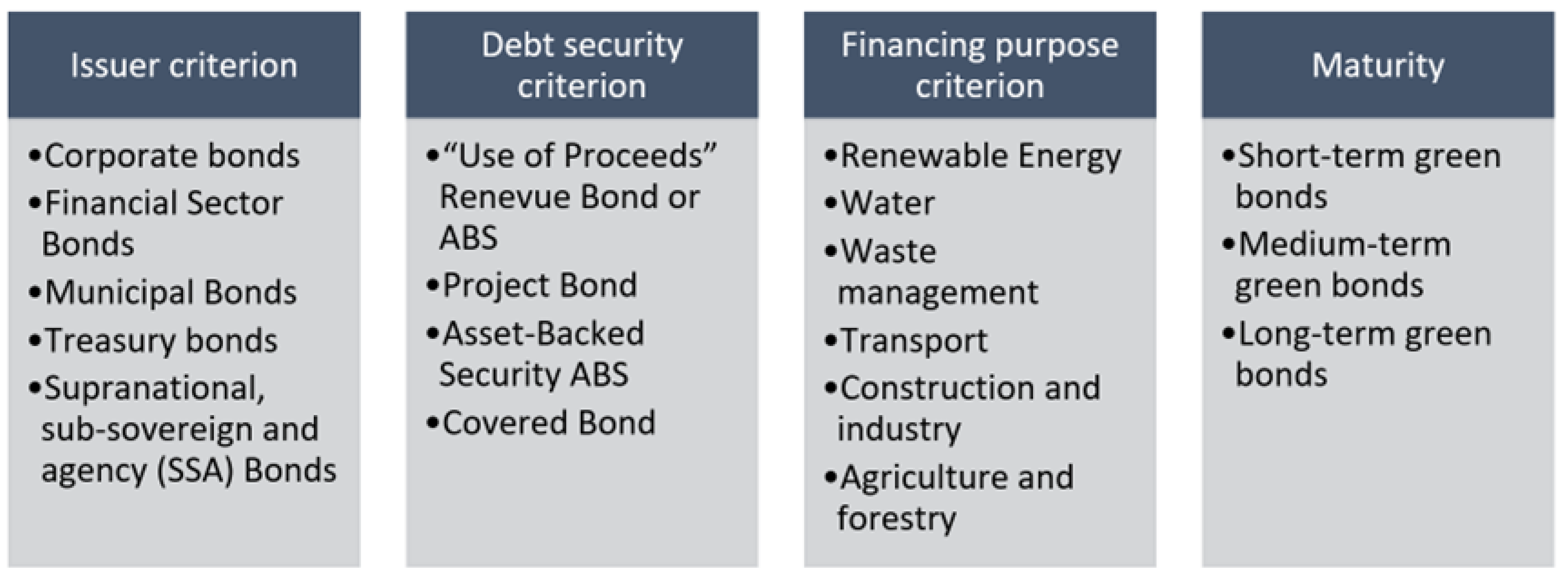

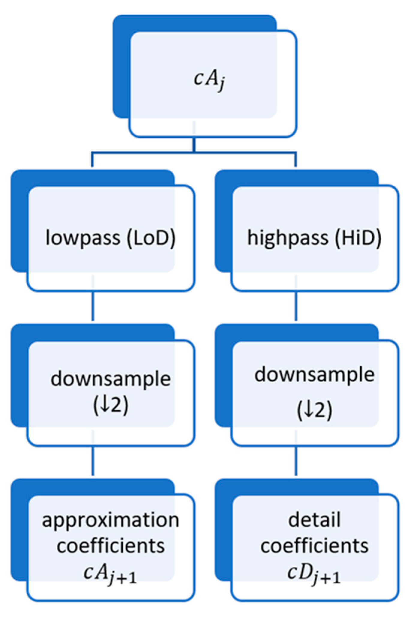


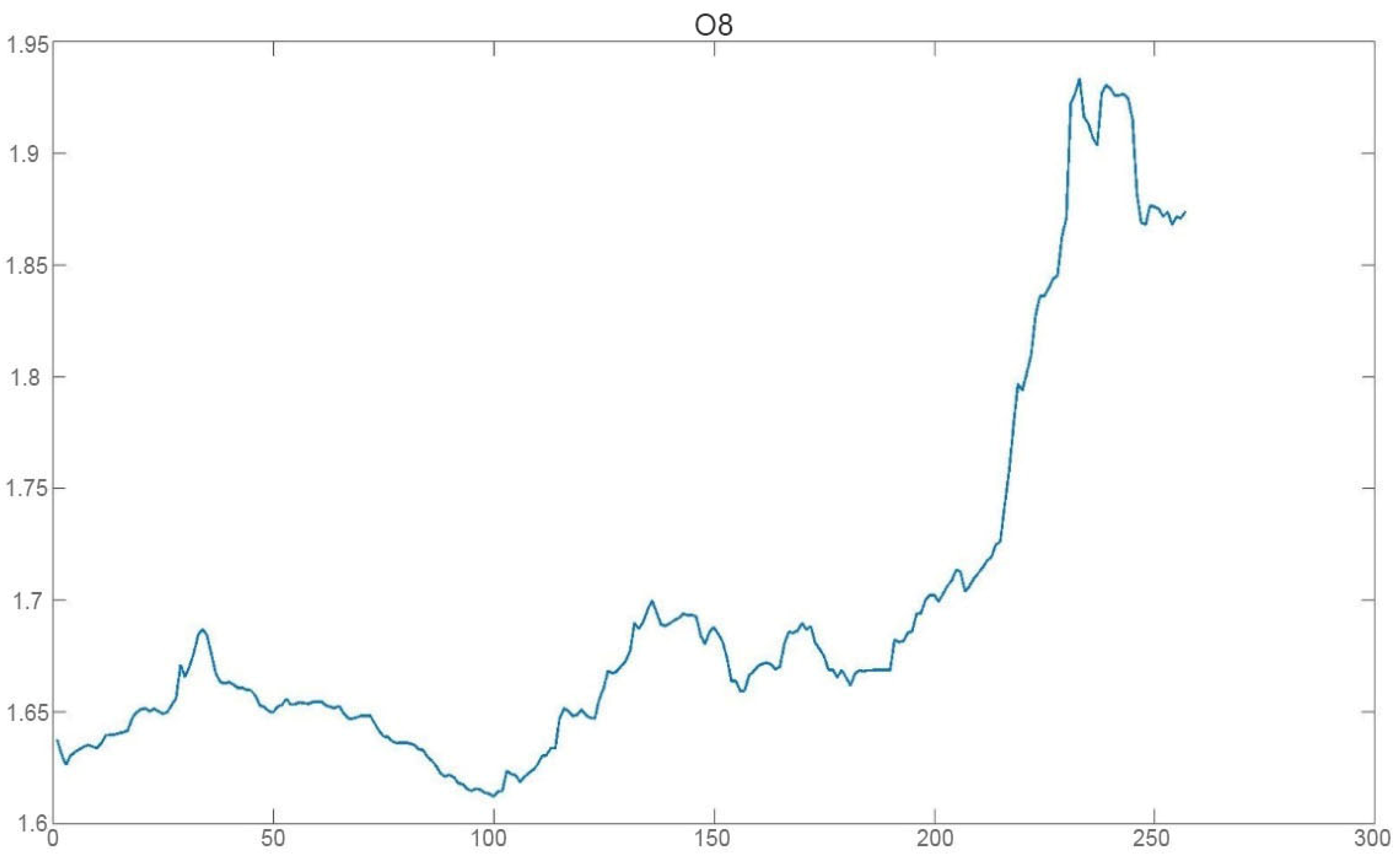
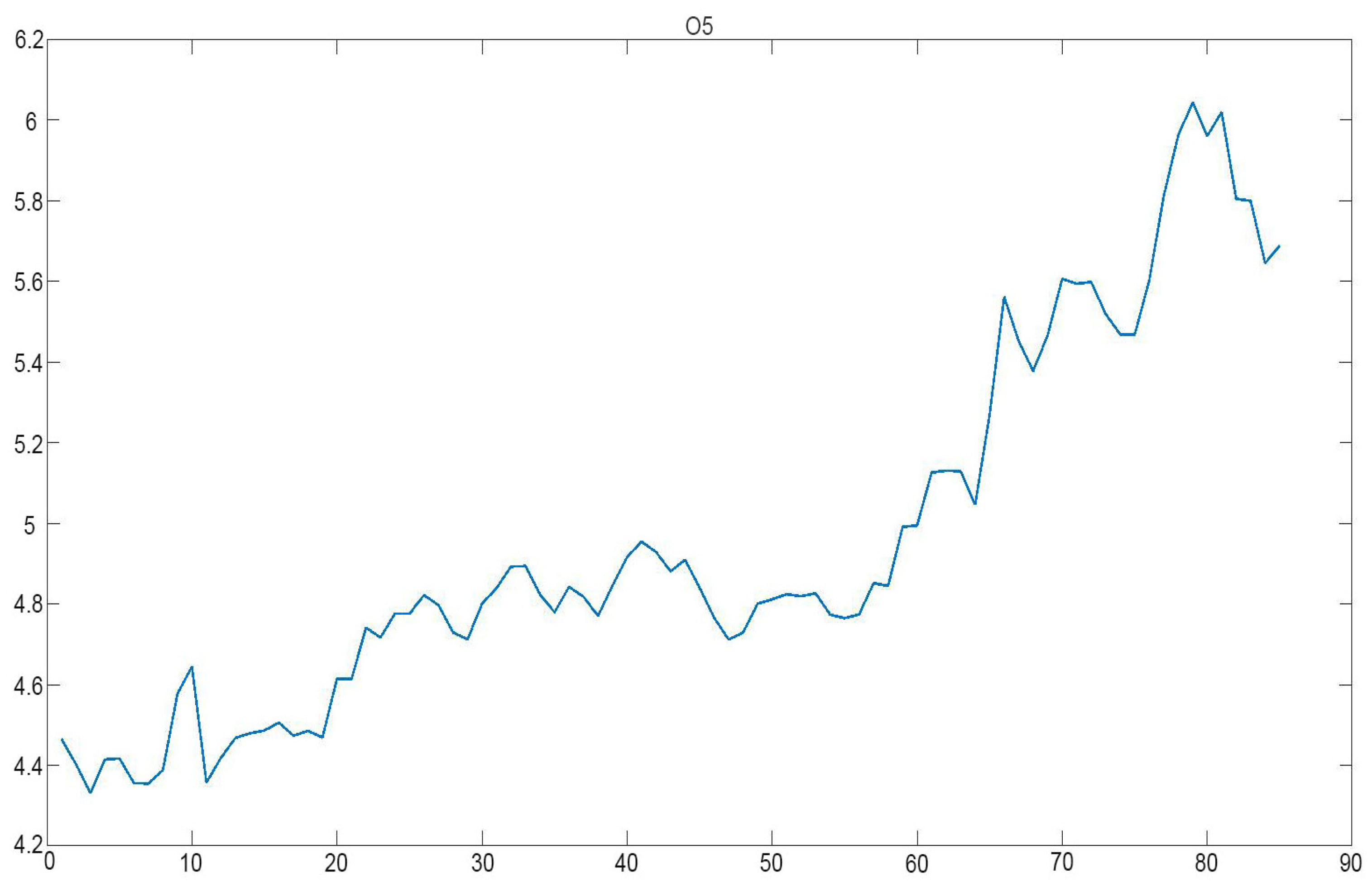
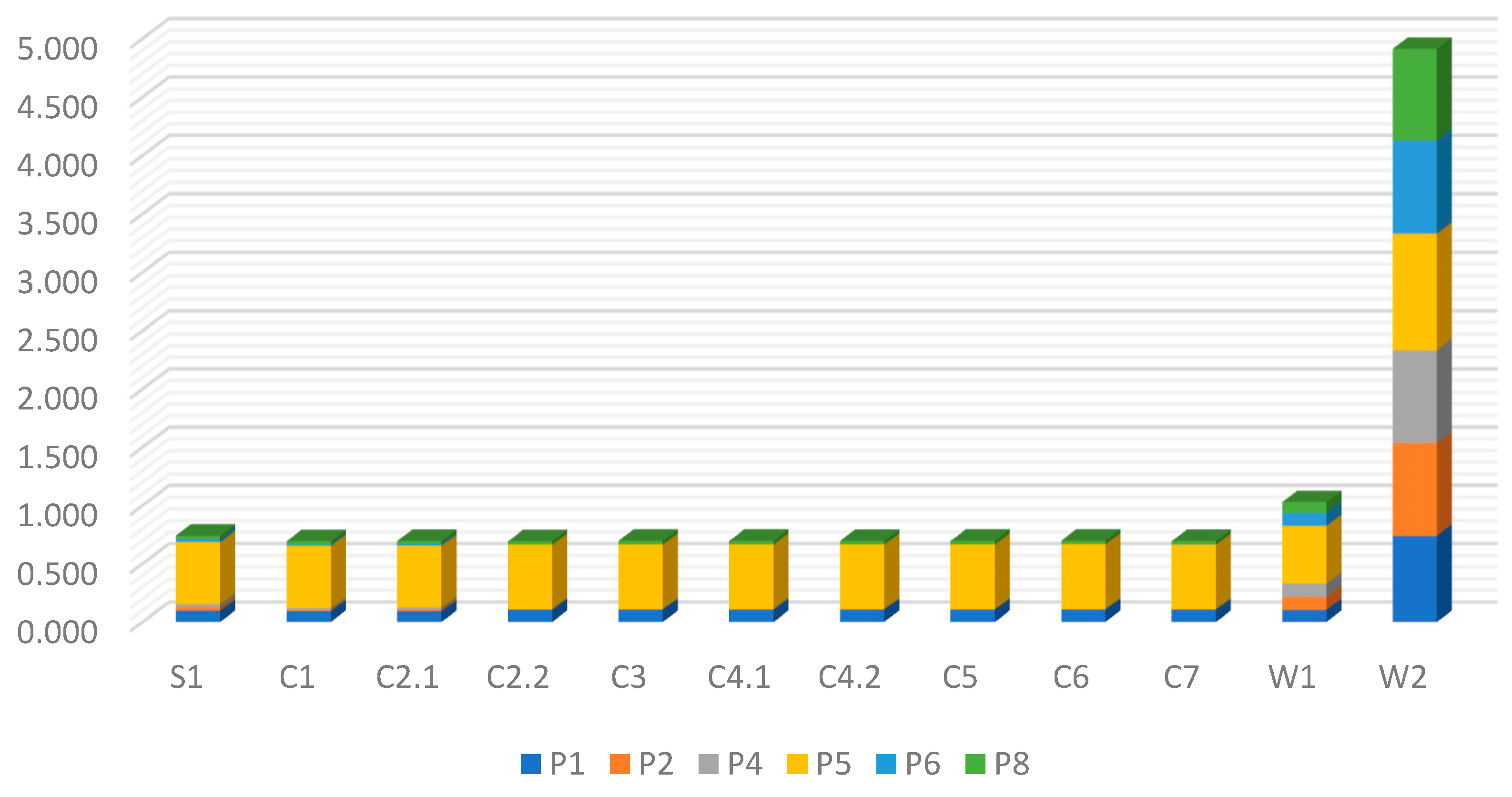


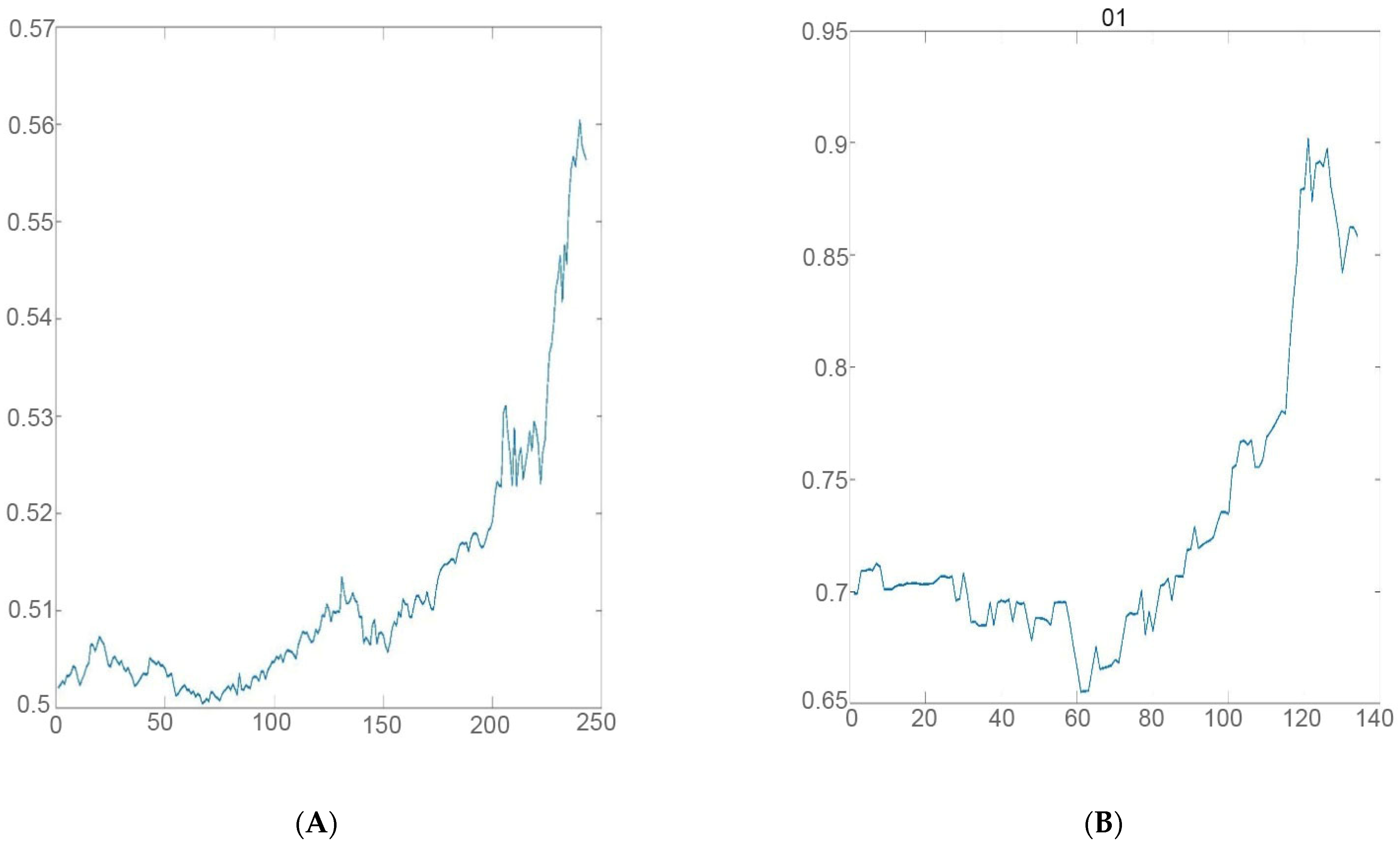
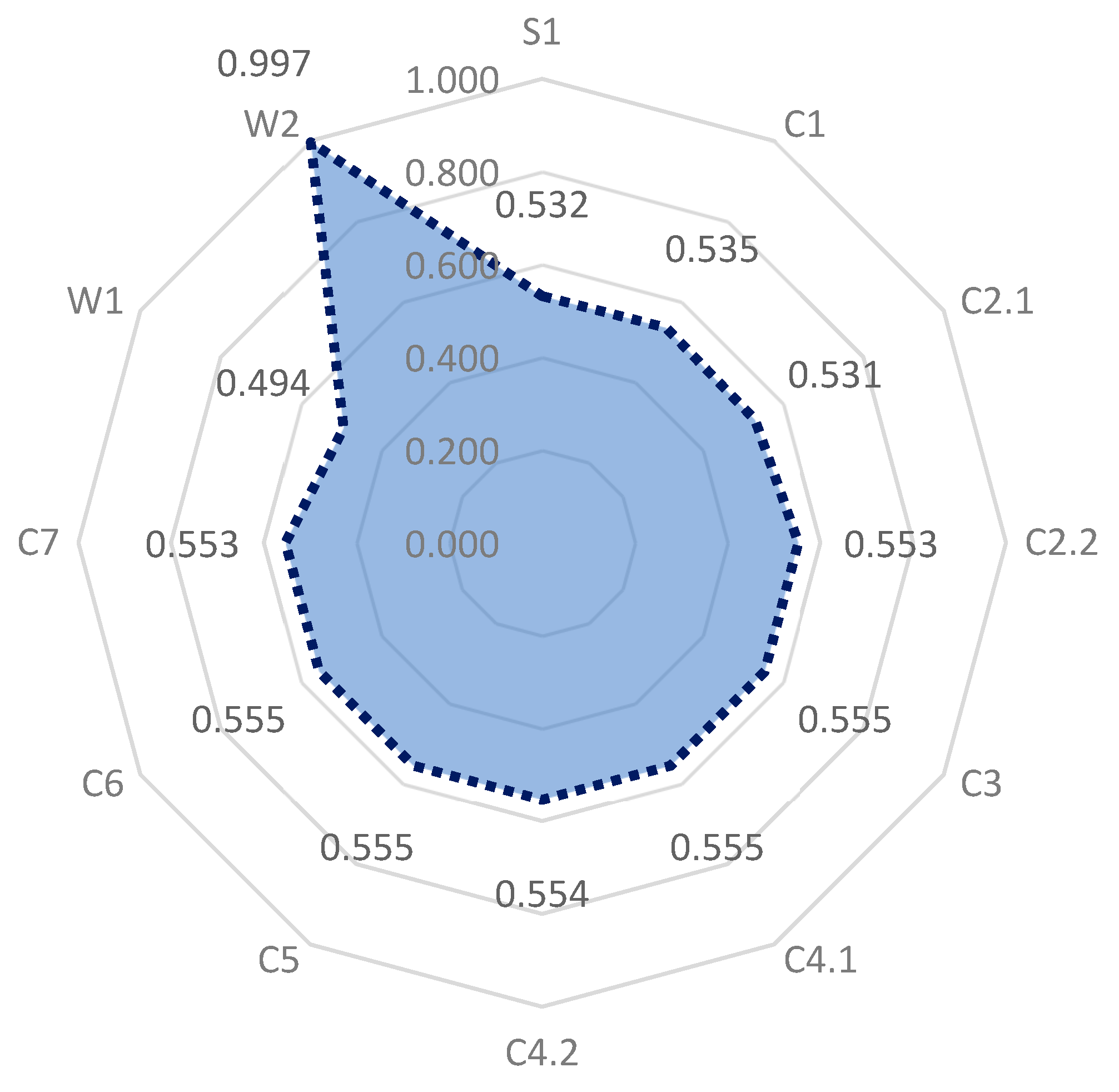

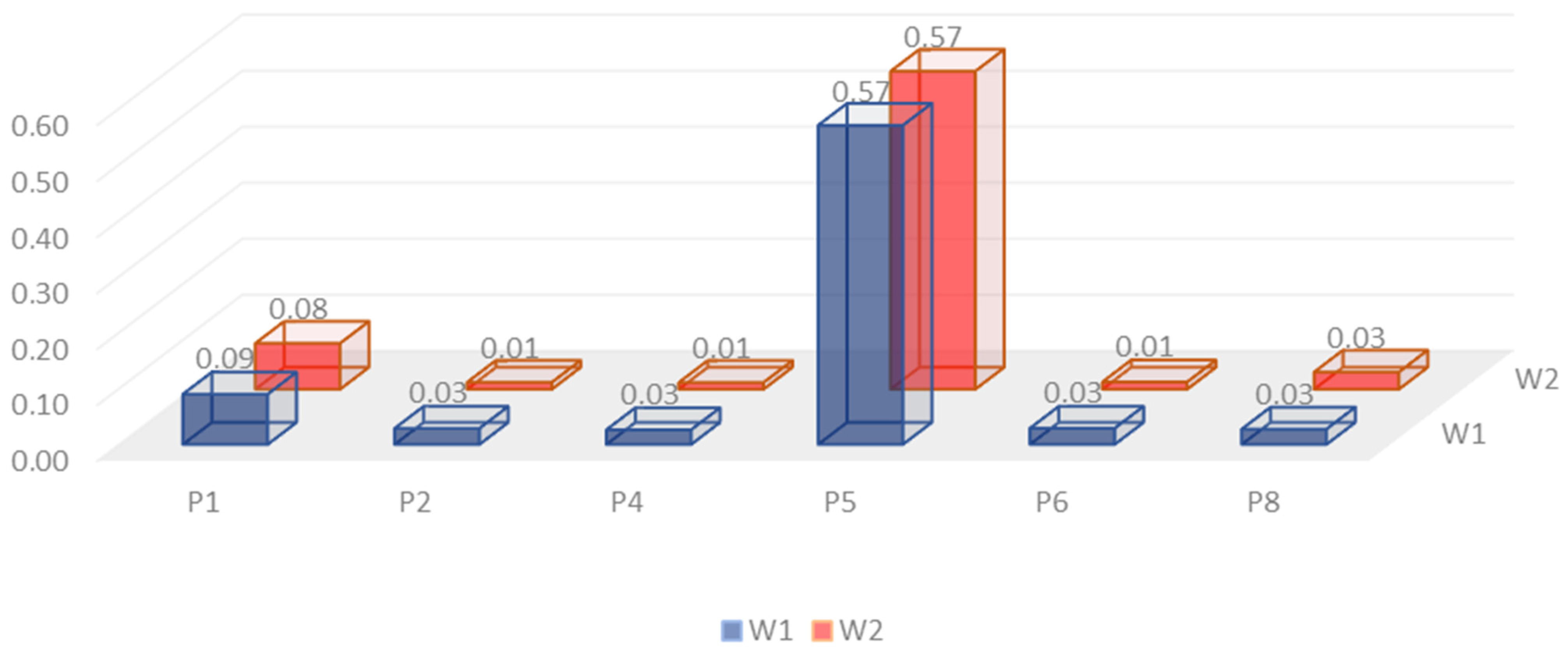


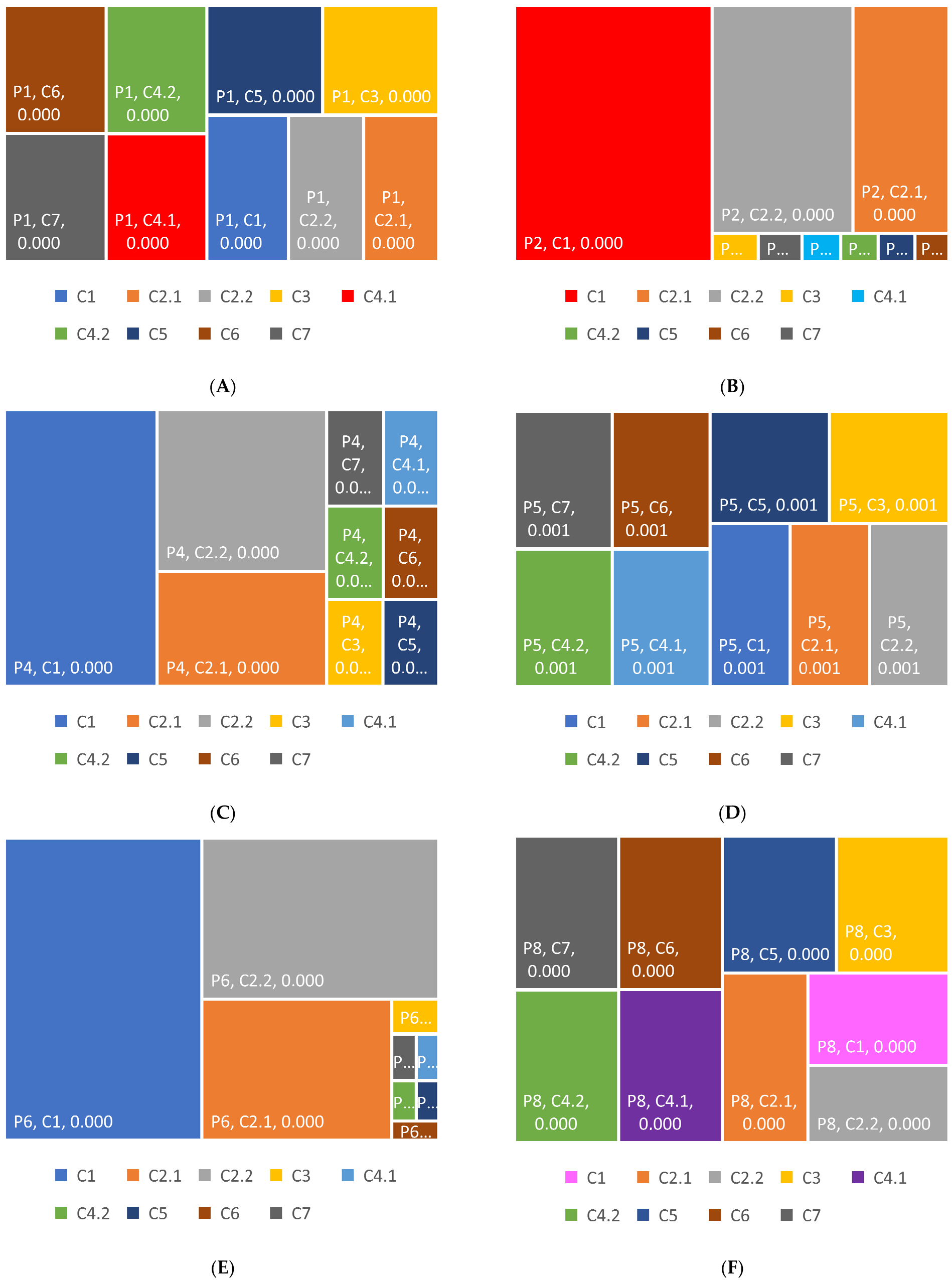


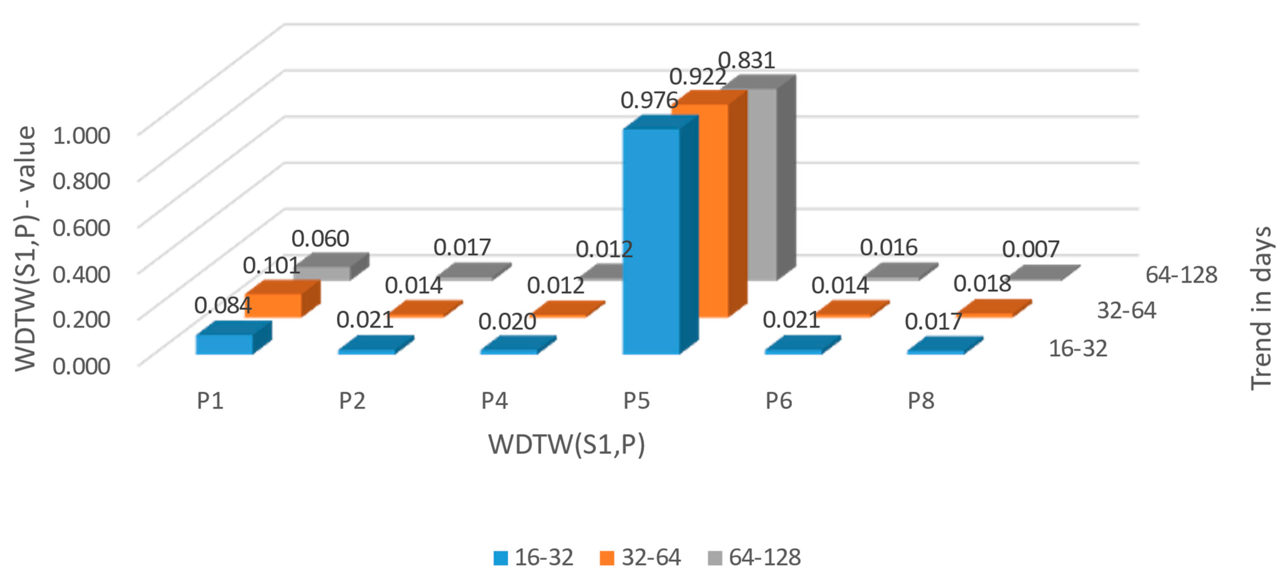
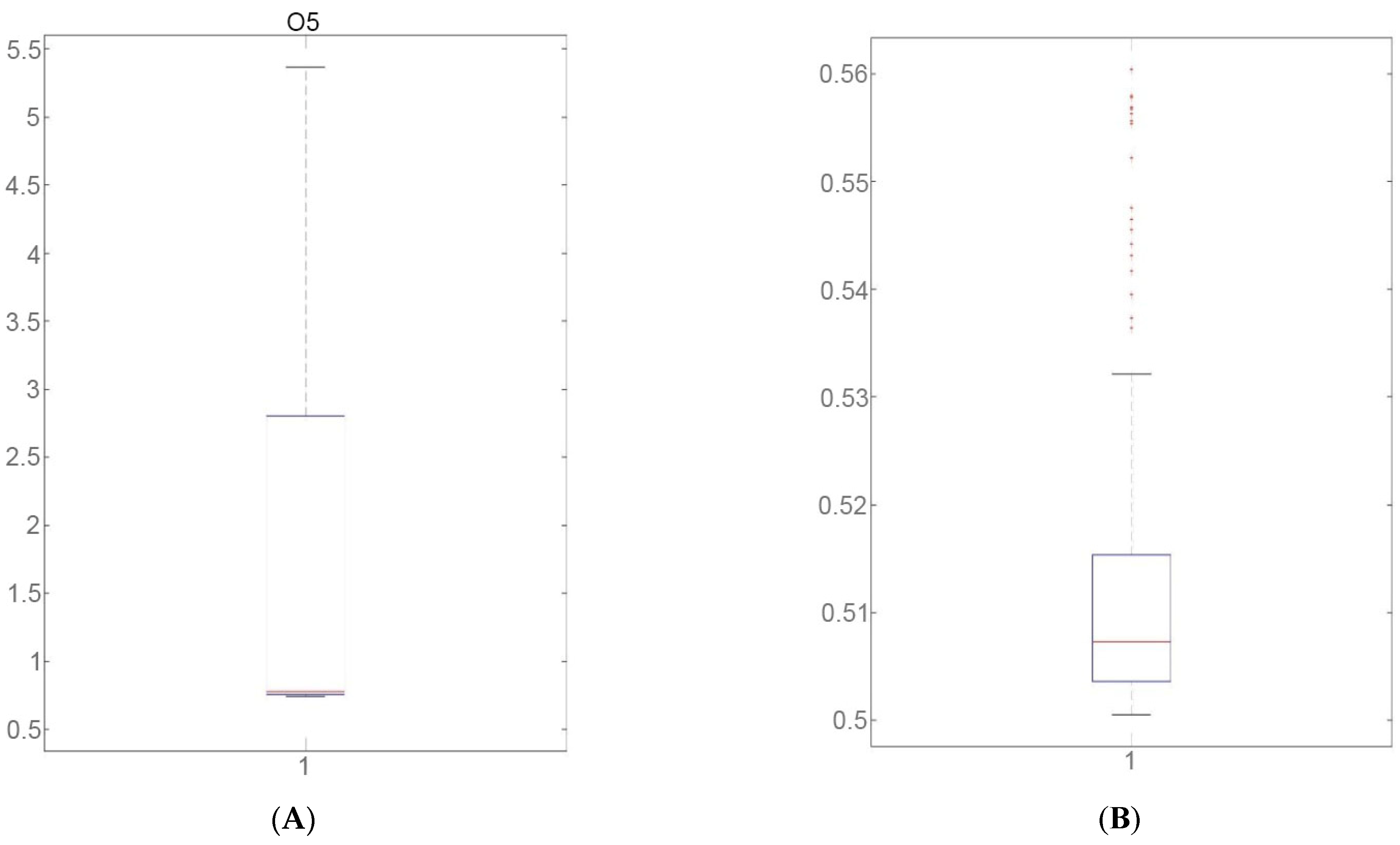
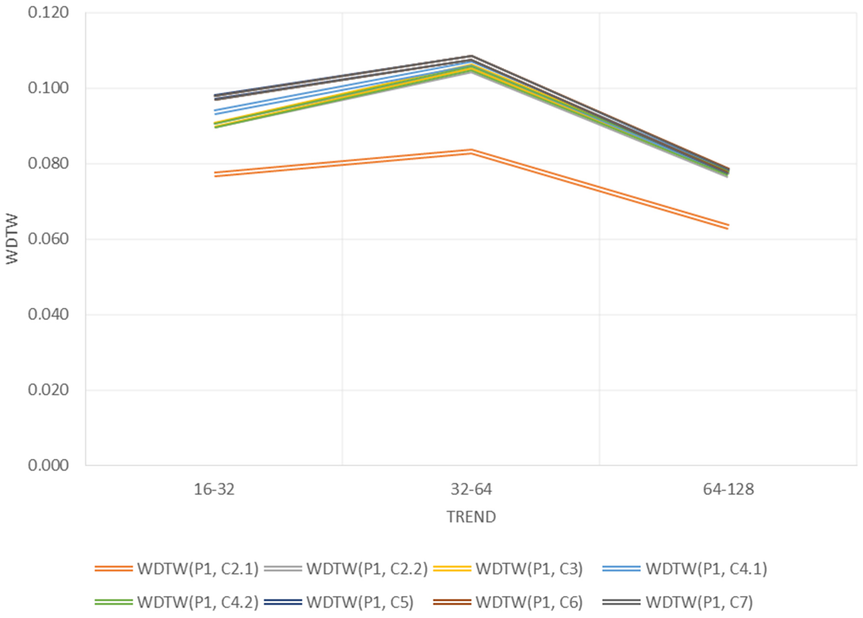
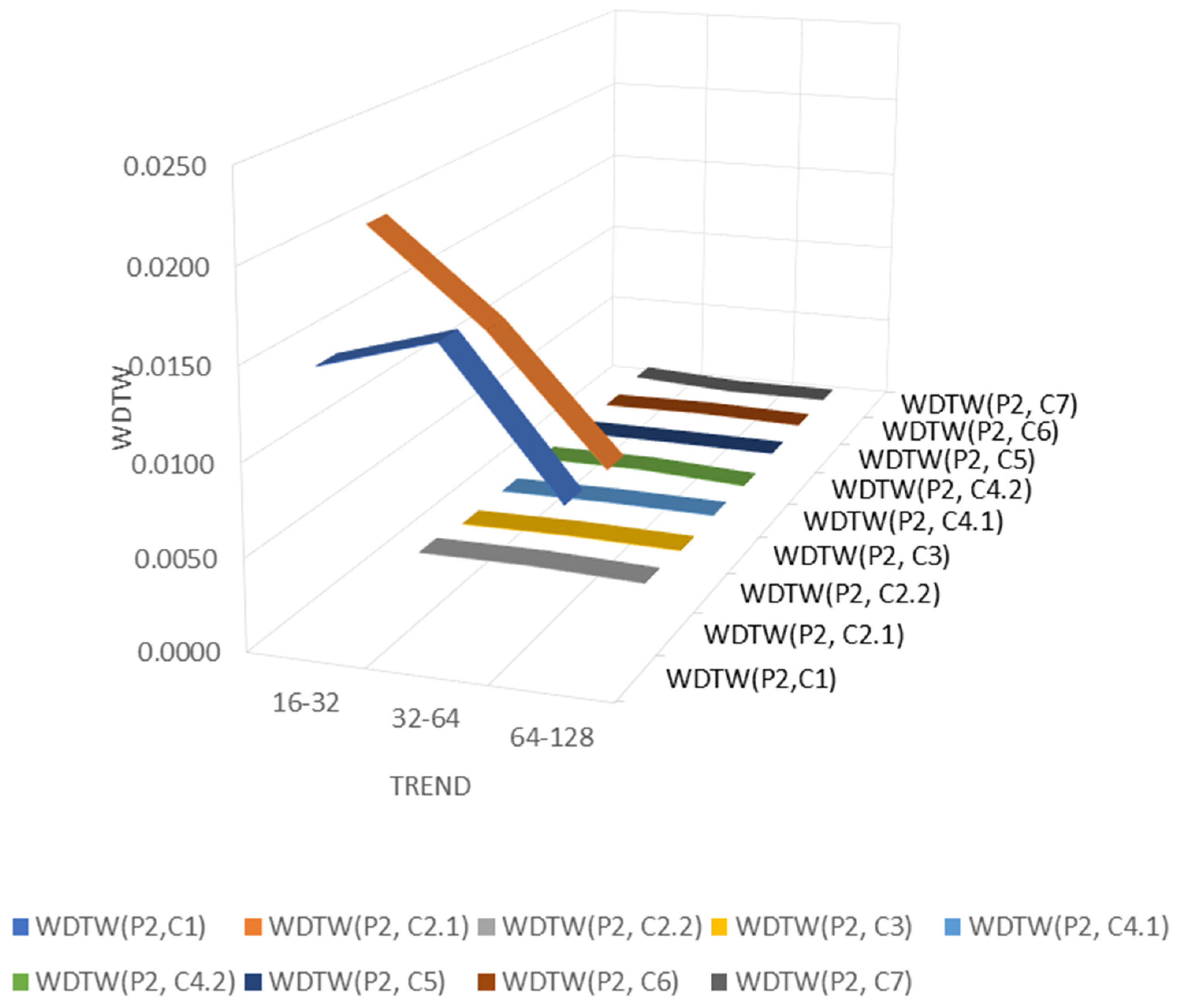
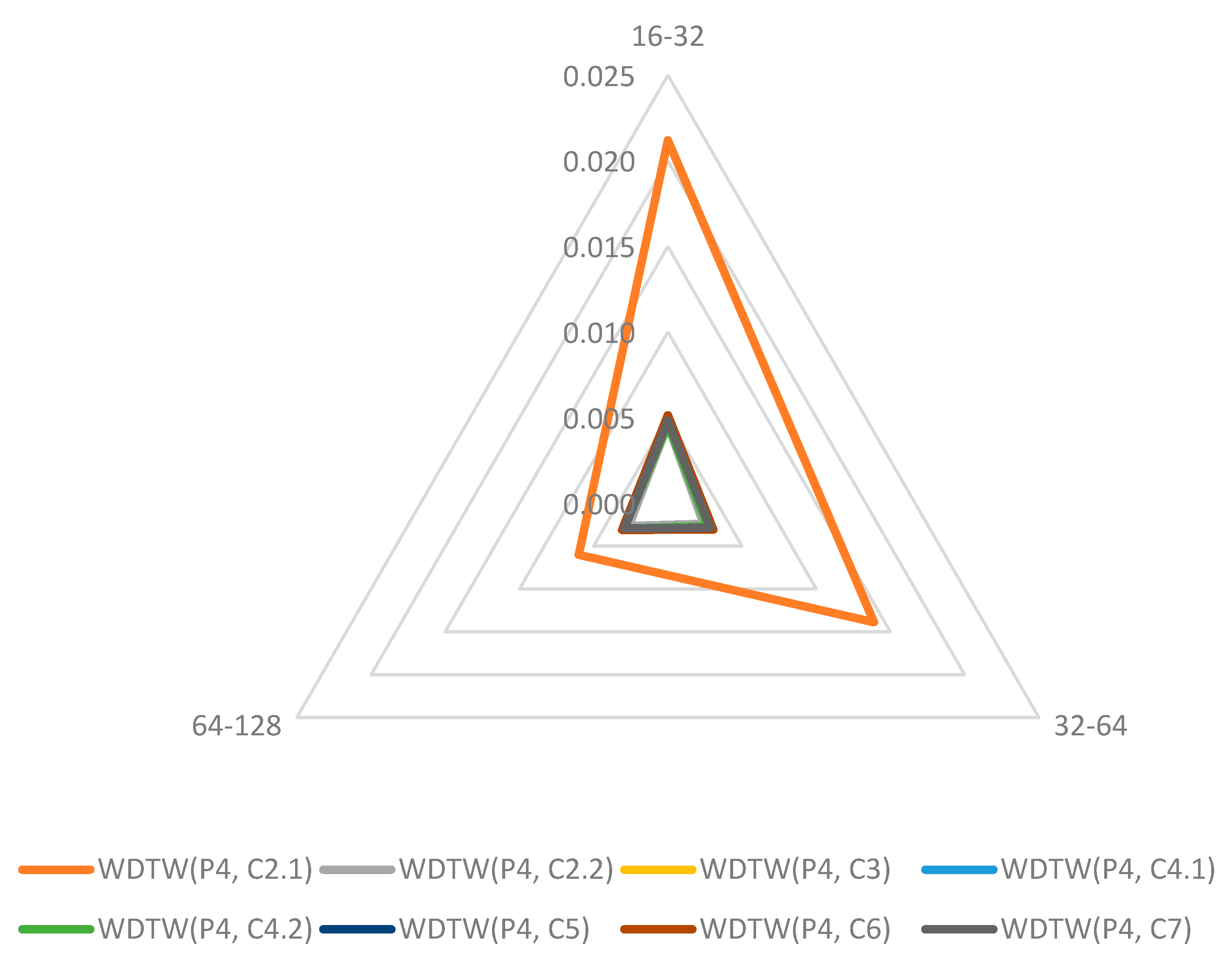
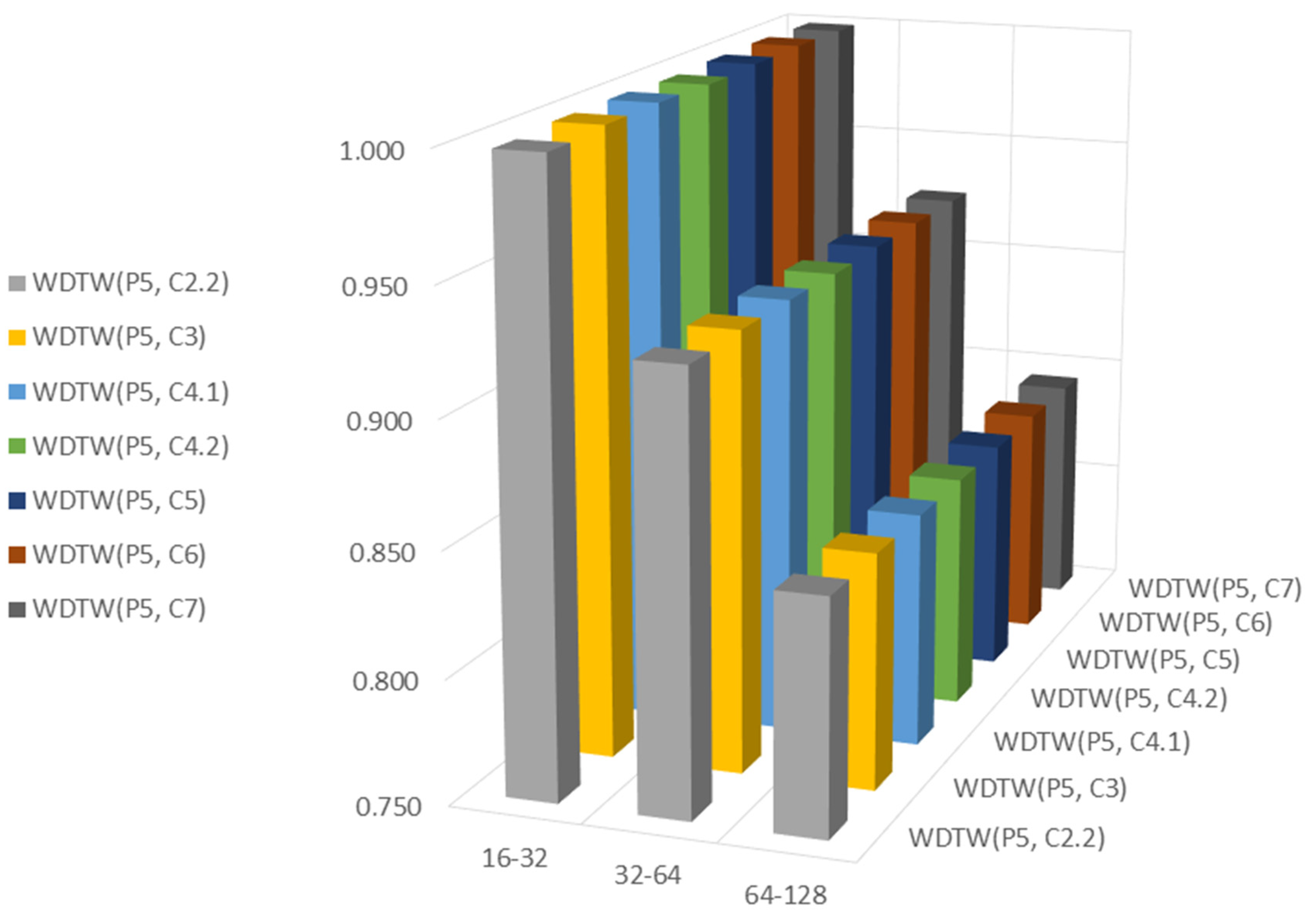


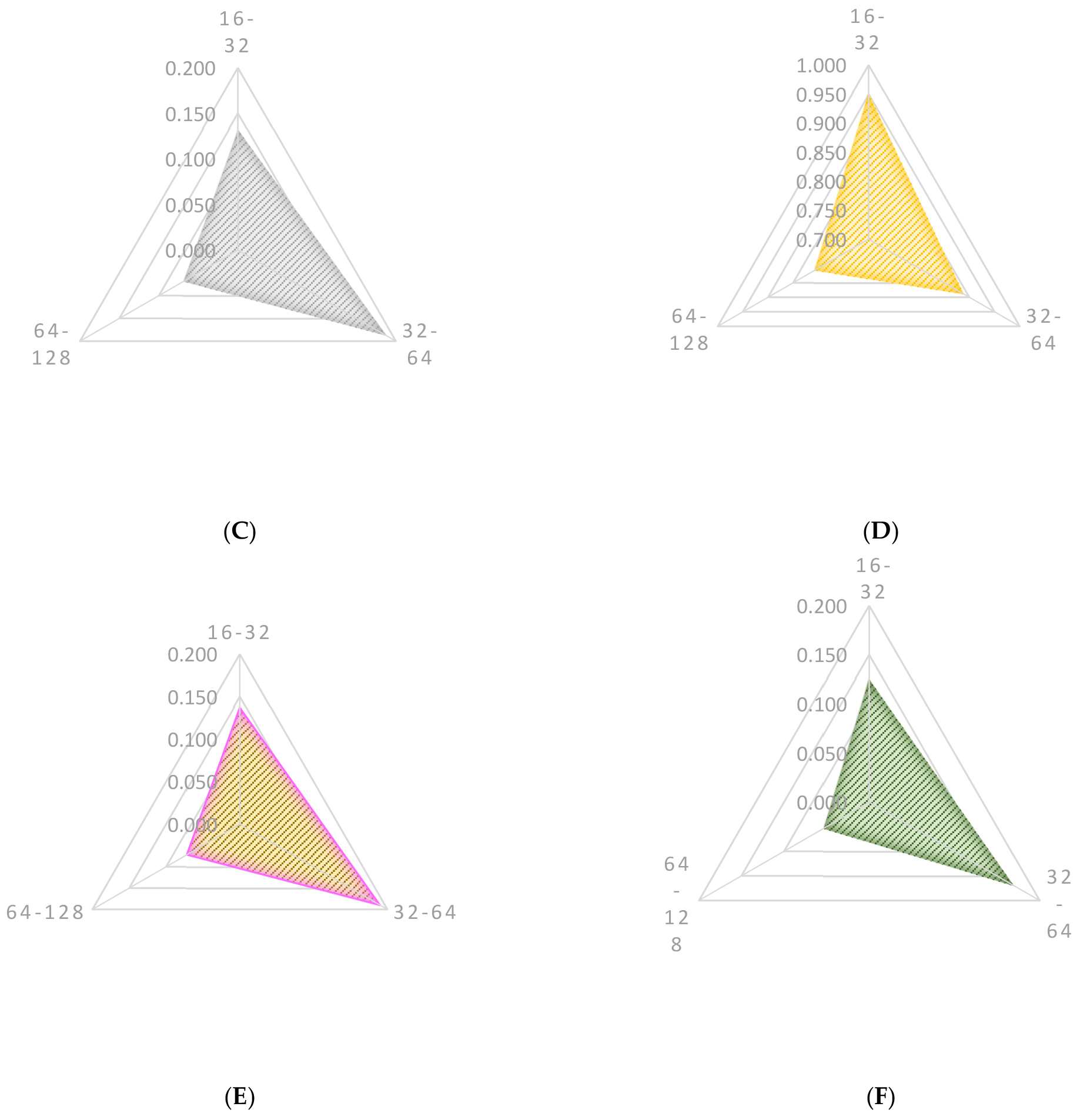
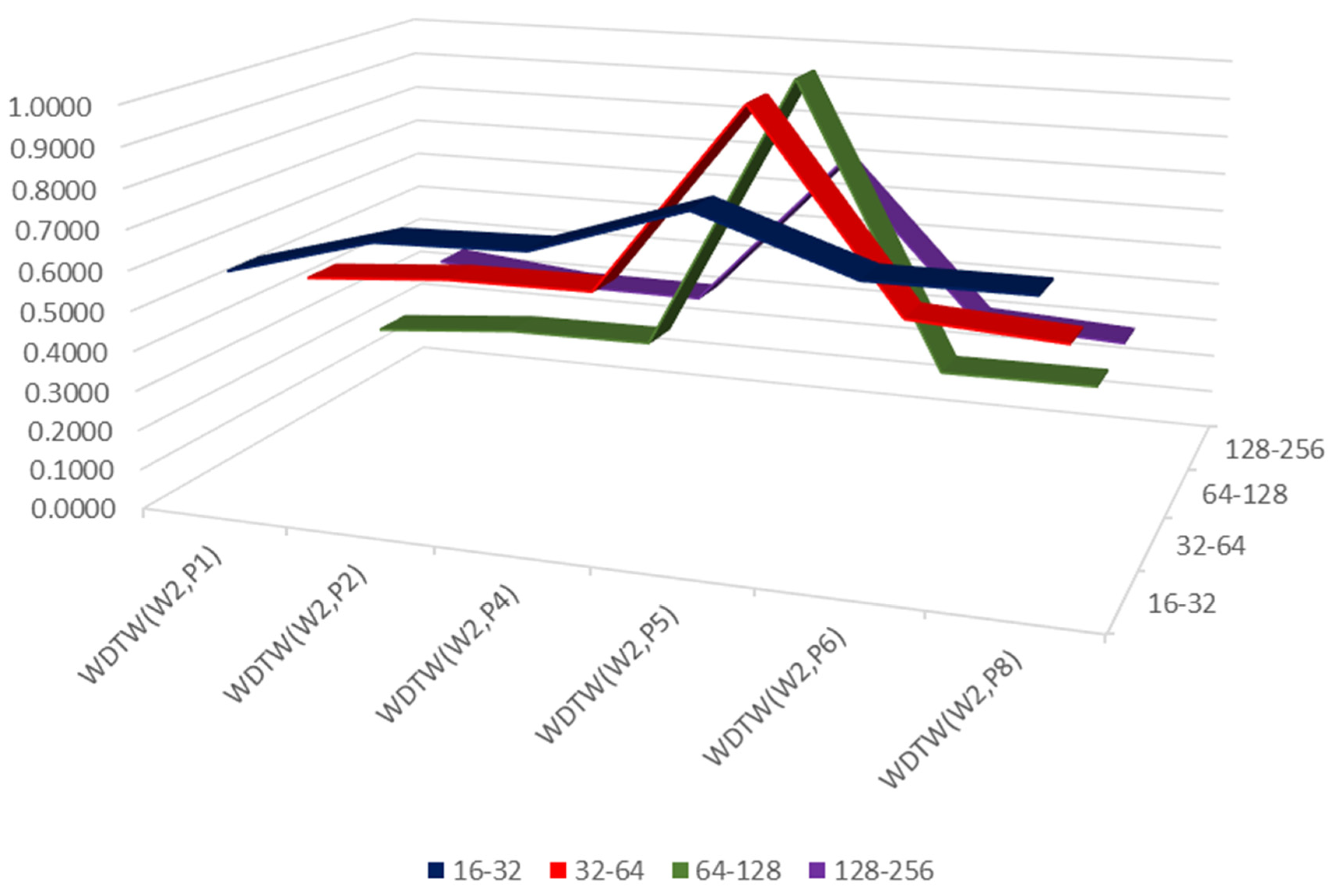
Disclaimer/Publisher’s Note: The statements, opinions and data contained in all publications are solely those of the individual author(s) and contributor(s) and not of MDPI and/or the editor(s). MDPI and/or the editor(s) disclaim responsibility for any injury to people or property resulting from any ideas, methods, instructions or products referred to in the content. |
© 2023 by the authors. Licensee MDPI, Basel, Switzerland. This article is an open access article distributed under the terms and conditions of the Creative Commons Attribution (CC BY) license (https://creativecommons.org/licenses/by/4.0/).