Abstract
This paper overviews our recent results of energy market modeling, including The option pricing formula for a mean-reversion asset, variance and volatility swaps on energy markets, applications of weather derivatives on energy markets, pricing crude oil options using the Lévy processes, energy contracts modeling with delayed and jumped volatilities, applications of mean-reverting processes on Alberta energy markets, and alternatives to the Black-76 model for options valuation of futures contracts. We will also consider the clean renewable energy prospective in Canada, and, in particular, in Alberta and Calgary.
Keywords:
energy markets; option pricing; mean-reverting assets; variance and volatility swaps; risk premia on energy markets; crude oil pricing; weather derivatives; Lévy processes; delayed and jumped volatilities; Alberta energy markets; alternatives to the Black-76 model; wind, solar, and water energy 1. A Brief Introduction
In this paper, we provide an overview of some recent results of energy markets modeling, and consider the clean renewable energy prospective in Canada and, in particular, in Alberta. This brief introduction gives a quick insight into the eight papers on energy markets modeling we published during the period of 2008–2021.
Some commodity prices, such as oil and gas, exhibit mean reversion, unlike stock price. This means that they tend, over time, to return to some long-term mean. We presented an explicit option pricing formula for a mean-reverting asset in the energy market in the paper Swishchuk (2008).
We calculated the variance and volatility swaps on energy markets in Swishchuk (2013b).
We used future contracts written on temperature to demonstrate the hedging strategies for commodities as an application of weather derivatives in Cui and Swishchuk (2015). Our focus was on the dynamic hedging strategy of energy futures using temperature futures and constructing the hedge ratio.
Crude oil prices exhibit significant volatility over time and the distribution of returns on crude oil prices show at tails and skewness, and they barely follow normal distribution. This is the reason we use normal inverse Gaussian process, jump diffusion process, and variance-gamma process as three Lévy processes that do not have these drawbacks, and their tails carry heavier mass than normal distribution. Our results indicate that all these three Levy processes have very good out-of-sample results for near-at-the-money options compared to others (see Shahmoradi and Swishchuk 2016).
We also considered stochastic modeling and pricing of energy markets’ contracts for stochastic volatilities with delay and jumps. Our model of stochastic volatility exhibits jumps and also past dependence: the behavior of a stock price right after a given time t not only depends on the situation at but also on the whole past (history) of the process up to time The basic products in these markets are spot, futures and forward contracts and options written on these. We study forwards and swaps. A numerical example is presented for stochastic volatility with delay using the Henry Hub daily natural gas data (1997–2011); see Swishchuk (2020b).
In Lu et al. (2021), we introduced the fuel-switching price, which was designed for encouraging power plant companies to switch from coal to natural gas when they produce electricity and was successfully applied from the European market to the Albertan Market. Moreover, we introduced the energy-switching price, which considers the power switch from natural gas to wind. We modeled these two prices using five mean reverting processes including Regime-switching processes, Levy-driven Ornstein–Uhlenbeck process and Inhomogeneous Geometric Brownian Motion, and estimate them based on multiple procedures such as Maximum likelihood estimation and expectation–maximization algorithm. Finally, this paper proves the previous result applied on the Albertan Market that showed that the jump modeling technique is needed when modeling fuel-switching data. In addition, it not only provides a promising conclusion on the necessity of introducing regime-switching models to the fuel-switching data, but also shows that the regime-switching model is better fitted to the data.
In March 2020, the prompt month WTI futures contract settled below zero for the first time in the contract’s history. Many market participants apply the Black-76 model or some variation when calculating the value of the options on this futures contract as a relatively straightforward, parametric valuation method. This calculation model is hard wired into many commodity trading and risk management systems when the prices drop below zero, and traders and risk managers rely on its straightforward and reproducible output. However, Black 76 requires positive underlying market prices. The negative prompt month settlement price caused considerable consternation among energy traders and risk managers. More generally, OTC options are also available on basis or differential prices. These transactions are options on the difference between two published indexes such as NYMEX Henry Hub and AECO (for natural gas) or Cushing WTI and Houston (for crude oil). As such, these instruments frequently have negative underlying market prices. Our task was to propose alternative models to Black-76 to valuate option prices when the underlying future contracts can assume negative values. The paper Swishchuk et al. (2021), considers some alternatives to Black-76 model to value European options on future contracts in which the underlying market prices can be negative or/and mean reverting. We specifically consider two models, namely Ornstein–Uhlenbeck (OU) for negative prices and continuous-time GARCH (or inhomogeneous geometric Brownian motion) for positive prices. We then analyze the results and compare them with Black-76, the most commonly used model, when the underlying market prices are positive. Numerical examples are presented using WTI and NYMEX NG datasets.
Finally, we present a vision to transition to wind, water, and solar energy in Canada. A group of U.S. civil engineering has calculated that Canada could be completely powered by renewable energy, if they simply decide to do it. This group has said this would save billion CAD on health care costs every year and prevent 9884 annual air pollution deaths. Their research is available at TheSolutionsProject (2023).
This paper organized as follows. The option pricing formula for a mean-reversion asset is considered in Section 2. Variance and volatility swaps valuations on energy markets are presented in Section 3. Applications of weather derivatives on energy markets are reviewed in Section 4. Pricing crude oil options using Levy processes is considered in Section 5. Energy contracts modeling with delayed and jumped volatilities is presented in Section 6. Applications of mean-reverting processes on Alberta energy markets are reviewed in Section 7. Alternatives to the Black-76 model for options valuation of futures contracts are considered in Section 8. A vision to transition to wind, water, and solar energy in Canada is considered in Section 9. Predictions of future wind and solar energy in Alberta are presented in Section 10. Description of the Energy Transition Centre in Calgary, AB, Canada, is mentioned in Section 11. A discussion is presented in Section 13. Section 12 concludes the paper.
Literature Review
Zonal and nodal models of energy market in European Union were considered in Borowski (2020). The competitive behavior of hydroelectric power plants under uncertainty in the spot market was studied in De Brito et al. (2022). A review of an offline and online approach to the OLTC condition monitoring was considered in Ismail et al. (2022). Modeling, optimization, and analysis of a virtual power plant demand response mechanism for the internal electricity market considering the uncertainty of renewable energy sources were studied in Ullah et al. (2022). Strategies for increasing the grid-integrated share of renewable energy with energy storage and existing coal fired power generation in China were considered in Zhao et al. (2022). A novel energy management optimization method for commercial users based on hybrid simulation of electricity market bidding was studied in Wang et al. (2022). Identification of generators’ economic withholding behavior based on a SCAD-logit model in electricity spot market was considered in Sun et al. (2022). Multi-objective optimal power flow solution using a non-dominated sorting hybrid fruit fly-based artificial bee colony was studied in Mallala et al. (2022). Possible pathways toward carbon neutrality in Thailand’s electricity sector by 2050 through the introduction of H2 blending in natural gas and solar PV with BESS was considered in Diewvilai and Audomvongseree (2022). Potential benefits for residential buildings with photovoltaic battery system participation in peer-to-peer energy trading were studied in Zhang et al. (2022). An optimization model for the integration of the electric system and gas network in Peru was considered in Navarro et al. (2022). Structural and operating features of the creation of an interstate electric power interconnection in North-East Asia with large-scale penetration of renewable energy was studied in Podkovalnikov et al. (2022). Long-term commitments to replace electricity generation with SMRs and estimates of climate change impact costs using a modified VENSIM dynamic integrated climate economy (DICE) model were studied in Shobeiri et al. (2022).
We note that some relevant papers may also be found in https://www.mdpi.com/topics/energy_market_power_system (accessed on 23 June 2023) and in https://www.mdpi.com/1996-1073/13/16/4182 (accessed on 23 June 2023).
2. Closed-Form Option Pricing Formula for a Mean-Reverting Asset on the Energy Market (Swishchuk 2008)
A risky asset following the mean-reverting stochastic process is given by the following stochastic differential equation:
where: W is a standard Wiener process, is the volatility, the constant L is called the ‘long-term mean’ of the process, to which it reverts over time, and measures the ‘strength’ of the mean reversion.
This mean-reverting model is a one-factor version of the two-factor model made popular in the context of energy modeling by Pilipović (1998). We call it continuous-time GARCH or the inhomogeneous geometric Brownian motion model.
Using a change of time method, we find an explicit solution of this Equation (1), and using this solution, we are able to find the variance and volatility swaps pricing formula under the physical measure. Then, using the same argument, we find the option pricing formula under risk-neutral measure. The option pricing formula has the following expression:
where
is the solution of the following equation:
and is the probability distribution , i.e., cdf of r.v.:
however, instead of a, we have to take is a market price of risk. We note that this cdf can be estimated and calculated with the method used in Yor (1992); see also Yor and Matsumoto (2005). Change of time for diffusion equations was also developed in Ikeda and Watanabe (1981).
Remark 1.
When and then the explicit option pricing formula (2) is the well-known Black–Scholes formula.
Numerical Example (AECO Natural GAS Index (1 May 1998–30 April 1999))
We shall calculate the value of a European call option on the price of a daily natural gas contract. To apply our formula for calculating this value we need to calibrate the parameters , and λ. These parameters may be obtained from futures prices for the AECO Natural Gas Index for the period 1 May 1998 to 30 April 1999 (see Bos et al. 2002, p. 340). The parameters pertaining to the option are presented in Table 1 below. The Figure 1 and Figure 2 show dependence and on and respectively, and dependence of European call option on

Table 1.
Price and option process parameters, obtained from futures prices for the AECO Natural Gas Index for the period 1 May 1998 to 30 April 1999 (see Bos et al. 2002, p. 340).
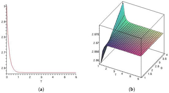
Figure 1.
(a) Dependence of on T (AECO Natural Gas Index (1 May 1998–30 April 1999)). (b) Dependence of on and T (AECO Natural Gas Index (1 May 1998–30 April 1999)).
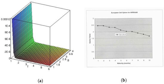
Figure 2.
(a) Dependence of variance of on and T (AECO Natural Gas Index (1 May 1998–30 April 1999)). (b) Dependence of European call option price on maturity (months) ( and ) (AECO natural gas index (1 May 1998–30 April 1999)). Remark: e.g., in the figure means
For the value of , we can take
3. Variance and Volatility Swaps on Energy Markets (Swishchuk 2013a, 2013b)
Variance swaps are quite common in commodity, e.g., on energy markets, and they are commonly traded. We consider the Ornstein–Uhlenbeck process for a commodity asset with stochastic volatility following the continuous-time GARCH model or the one-factor model Pilipović (1998). The classical stochastic process for the spot dynamics of commodity prices, as mentioned above, is given by Schwartz’ model (see Schwartz 1997). It is defined as the exponential of an Ornstein–Uhlenbeck (OU) process, and has become the standard model for energy prices possessing mean-reverting features.
We consider a risky asset on energy markets with stochastic variance following a mean-reverting stochastic process satisfying the following SDE (continuous-time GARCH(1,1) model):
where: is a standard Wiener process, L is the mean reverting level (or equilibrium level), a is the speed of mean reversion, and is the volatility of volatility Applying a change of time method, we find an explicit solution of this equation, and using this solution, we are able to find the variance and volatility swaps pricing formula under the physical measure. Then, using the same argument, we find the option pricing formula under a risk-neutral measure. We applied the Brockhaus-Long approximation (see Brockhaus and Long 2000) to find the value of the volatility swap. A numerical example for the AECO Natural Gas Index for the period 1 May 1998 to 30 April 1999 is presented.
The risk-neutral stochastic volatility model (compared with (3)) has the following form:
where
and is the market price of risk.
For the variance swap, we have (using (4) and the change of time method):
For the volatility swap, we obtain the convexity adjustment formula:
Numerical Example (AECO Natural Gas Index for the Period 1 May 1998 to 30 April 1999)
Table 2.
Parameter values.
For the value of , we can take
For variance swap and for volatility swap with risk-adjusted parameters, we use the formula obtained above. Figure 3, Figure 4 and Figure 5 below display variance and volatility swaps for different cases.
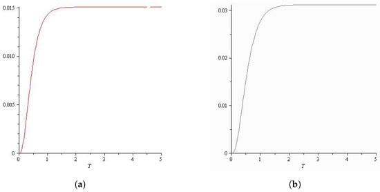
Figure 3.
(a) Variance Swap. (b) Volatility Swap.
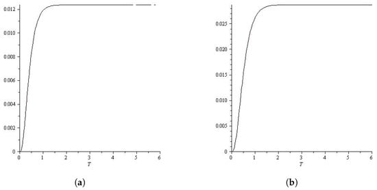
Figure 4.
Variance and volatility swaps on energy markets: Figures Swishchuk (2013b). (a) Variance swap (risk-adjusted parameters). (b) Volatility swap (risk-adjusted parameters).
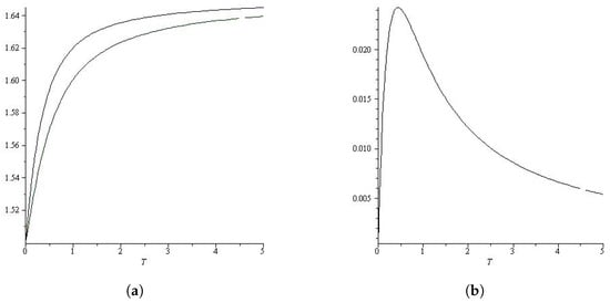
Figure 5.
Variance and volatility swaps on energy markets: Figures Swishchuk (2013b). (a) Comparison: adjusted and non-adjusted price. (b) Convexity adjustment.
4. Weather Derivatives on Energy Markets (Swishchuk and Cui 2013 and Cui and Swishchuk 2015)
For the weather derivatives market, contracts written on weather indices first appeared over the counter (OTC) in July 1996 between Aquila Energy and Consolidated Edison Co. from the United States. After that, companies accustomed to trading weather contracts based on electricity and gas prices in order to hedge their price risks realized by weather during the end of 1990s and the beginning of 2000s. Thus, the market grew rapidly and expanded to other industries and to Europe and Japan. Following the prosperous boom of the weather financial market, many academic papers, such as Considine (2000) and Hamisultane (2006), started to put their attention on the modeling and pricing of weather derivatives. The earliest references written in the field of the weather derivatives are Ellen (1998) and Kaminski (1998).
Weather affects different entities in different ways. In order to hedge these different types of risks, weather derivatives are written on different types of weather variables or weather indices. The most commonly used weather variable is temperature. Widely used temperature indices include cumulative average temperature (CAT), heating degree days (HDD), and cooling degree days (CDD). They are originated from the energy industry, and designed to correlate well with the local demands for heating or cooling.
CAT is defined as the sum of the daily average temperature over the period of the contract, where the index CAT: = where is the daily average temperature. It is mainly used in Europe and Canada. In winter, HDD is used to measure the demand for heating, i.e., it is a measure of how cold the weather is and is usually used in the United States, Europe, Canada, and Australia. In contrast, CDD is used in summer to measure the demand of energy used for cooling and as a measure of how hot the weather is. It is usually used in the United States, Canada, and Australia.
The definitions for HDD and CDD are given by HDD: = and CDD: = where the constant c denotes the threshold, say Since most air conditioners are switched on when temperatures are above or below
With respect to our model, consider the weather index which is the daily average temperature (DAT). We suppose the DAT has a generalization of the Ornstein–Uhlenbeck dynamics:
where is a Lévy process (jump-diffusion), is the seasonal mean level, and k is the speed in which the temperature reverts to is assumed to be a measurable and bounded function represents the seasonal volatility of temperature. In the simplest case, —a standard Wiener process.
This model was first introduced by Dornier and Queruel (2000) with Brownian motion as the random noise. Benth and Šaltytė-Benth (2005) has successfully applied this model with a generalized hyperbolic Lévy process to the Norwegian temperature data. We applied this model to our Canadian temperature data (Swishchuk and Cui 2013).
We define the temperature futures prices written on CAT, CDD, and HDD, which constitute the three main classes of futures products at the CME market. Consider the price dynamic of future written on CAT over specific time period with Firstly, assume the daily average temperature follows stochastic differential equation, with being a Lévy process and a constant continuously compounding interest rate r.
The future price at time based on CAT under risk-neutral probability measure Q is:
where Q is the risk-neutral measure (specified through Esscher transform) and is -algebra generated by
Similarly, the risk-neutral CDD and HDD future prices are defined as:
and
The relationship between futures prices of CAT, CDD, and HDD is defined as:
We use future contracts written on temperature to demonstrate the hedging strategies for commodities as an application of the weather derivative.
Within several forms of weather derivatives, the future contract does not require cost to enter a position, since when entering a future contract, the probability of weather event being lower or higher than the threshold is the same on both sides, where either side has the same chance of receiving payoff from the counter party.
There are two types of hedging strategies using temperature futures in the following contents: the first strategy is (a) static hedging, mainly focusing on mitigating the volume risk of commodity sales using temperature futures; the other strategy considers (b) the dynamic hedging strategy of commodity future using temperature futures:
- (a)
- In a static hedge, the number of hedging contracts is not changed over the course of the hedge in response to any movement in the values of the hedging instrument or the hedged asset.
- (b)
- In a dynamic hedge, on the other hand, more hedging contracts are bought or sold to bring back the hedge ratio to the target hedge ratio.
A hedge ratio is the ratio of exposure to a hedging instrument to the value of the hedged asset. A ratio of 1 or means that the position is fully hedged and a ratio of 0 means it is not hedged at all.
Without loss of generality, we choose the energy market as the one to hedge using temperature futures.
Therefore, our focus will be on the dynamic hedging strategy of energy futures using temperature futures. In the spirit of Broadie and Jain (2008), consider a portfolio at time t containing one unit of energy (e.g., heating oil) future and ( is the hedge ratio for energy future ) units of weather futures both with maturity (delivery) at time Assume the portfolio has value at time t and a constant risk-free interest rate r, then:
The portfolio is self-financing, so the change in this portfolio in a small amount of time is given by:
Hence, in order to dynamically hedge the energy future with maturity T, the stochastic component of portfolio vanishes, and the hedge ratio could be defined as:
with an assumption that . Therefore, from the last equation, to hedge energy futures, we are required to hold units in (5) of the temperature future at time t.
Therefore, we need to specify two models for energy and temperature futures so that we could obtain the explicit dynamics of energy and temperature futures, and hence, obtain a closed form of the hedge ratio . For futures pricing purpose, these models will be built on the underlings of futures, namely the energy spot price and the daily average temperature.
Our energy and temperature models under risk-neutral measure Q are:
and
where is the market price of risk and and are Brownian motions (with correlation ) w.r.t.
The combined Q dynamics system for energy futures and CAT futures is:
where and are the expectation and variance of the log-spot price Therefore:
where and are time-dependent constants defined as:
We choose crude oil (the world’s most actively traded commodity, and the NYMEX (CME) division light, sweet crude oil futures contract is the world’s most liquid forum for crude oil trading) futures as the one that we want to hedge using CAT futures. Followed by the calibration method described in Schwartz (1997), the log-future prices need to be rewritten as the standard state-space form and then applied to the Kalman filter to obtain the parameter set , and spot price series .
The data used to calibrate the energy future consist of daily generic observations of WTI light, sweet crude oil futures prices (these data are obtained from the Bloomberg financial service) with delivery periods in the first two front months. The WTI crude oil futures data used in calibration cover the CME exchange daily settlement prices ranging from 2 January 2001 to 31 December 2010, resulting in 2508 records for each future contracts set (this choice of dataset is consistent with that in Swishchuk and Cui (2013), which is 10 years of temperature data from 1 January 2001 to 31 December 2010 in Calgary, AB, Canada). There is no exact delivery date for each contract; instead, the CME contract specification defines a delivery period ranging from the first calendar day to the last calendar day of the delivery month. Thus, we simply assume that the delivery date for each contract is the first calendar day in the delivery month to calculate the time to maturity value
The Table 3 below presents the estimation results for the energy model applied to the WTI crude oil future price data. The last two parameters and are the diagonal entries of matrix with random noise
Table 3.
Estimation results for the energy model applied to the WTI crude oil future price data.
For the temperature market, we follow the calibration procedure described in Swishchuk and Cui (2013) to obtain the parameter set For illustration purposes, we choose the estimated parameters in Calgary as the ones under the temperature market to calculate the hedge ratio. Recall the calibration results for Calgary in Swishchuk and Cui (2013); we could obtain the parameter set in Calgary as follows:
- and annual seasonal volatility;
To calculate the correlation parameter we use the correlation between the filtered log-spot price and daily average temperature as a natural approximation to . By taking all the daily average temperature on the dates with future prices available, and calculating the correlation coefficient between log-spot prices and average temperature of these days over 10 years (from 2 January 2001 to 31 December 2010), we have the correlation . This correlation indicates a positive correlation between the log-spot price of crude oil and daily average temperature. With the calibrated parameters in energy model and temperature model, we could then calculate the dynamic hedge ratio explicitly. In Figure 6, below, we plot the initial hedge ratio along the crude oil future delivery time (in days) and initial log-spot price dimensions.
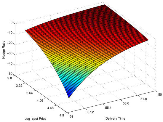
Figure 6.
Initial Hedge Ratio.
From Figure 6, we could find that if a person holds crude oil futures, initially, they need to short some CAT futures in the portfolio depending on the spot price of the crude oil and the time to delivery (trade termination) length. Basically, the number of temperature futures someone needs to hold will be more with longer time to delivery and higher spot price of crude oil. Moreover, we could conclude that the same effect holds for other energy commodities, such as heating oil, gas, and so on, since they are usually positively correlated with the crude oil market movement.
5. Pricing Crude Oil Options Using Lévy Processes (Shahmoradi and Swishchuk 2016)
Crude oil prices exhibit significant volatility over time and the distribution of returns on crude oil prices show fat tails and skewness, and they barely follow normal distribution. This is the reason we use the normal Gaussian process (NIG), jump diffusion process (JD), and variance-gamma process (VG) as three Levy processes that do not have these drawbacks and their tails carry heavier mass than normal distribution. We use fractional fast Fourier transform to calibrate parameters in an optimization setup, using data on European-style options on crude oil futures in NYMEX for the settlement date of 24th April 2015. Our results indicate that all these three Levy processes have very good out of sample results for near at the money options than others. Askari and Krichene (2008) used WTI crude oil spot prices from 2 January 2002 to 7 July 2006 in order to model oil price returns by employing Merton (1976) jump diffusion and VG processes. Crosby (2008) applied the jump-diffusion model for crude oil options on futures, while Madan and Seneta (1990) and Carr and Madan (1998) replicated this for stocks, where all forward option contracts had the same spot price.
We consider:
- Merton’s Jump diffusion model (JDM) (see Merton 1976):where Brownian motion and Poisson process are independent, .
- Normal inverse Gaussian (NIG) model:where is the drift under Q measure,is an NIG process, and is the inverse Gaussian process. The NIG process has three parameters, tail-heaviness skewness , and scale .
- Variance gamma (VG) model:where is a VG process such that:and is a gamma process with parameter
Figures, Tables, and Estimations are shown below. All Figures and Tables are cited from Shahmoradi and Swishchuk (2016), thus contains the captions from this paper. Figure 7 shows dependence of on T (AECO Natural Gas Index (1 May 1998–30 April 1999)).
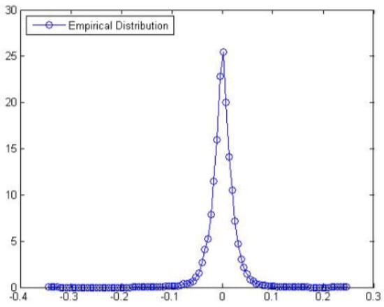
Figure 7.
Empirical Distribution of Returns on WTI Spot Crude Oil Prices. See Shahmoradi and Swishchuk (2016).
Table 4, Table 5 and Table 6 below describe WTI crude oil futures and options prices and calibrated parameters.
Table 4.
WTI Crude Futures and Options Prices with Strikes. See Shahmoradi and Swishchuk (2016).
Table 5.
WTI Crude Futures and Options Prices with Money-Ness. See Shahmoradi and Swishchuk (2016).
Table 6.
Calibrated Parameters of JDM, VG, and NIG Processes. See Shahmoradi and Swishchuk (2016).
Figure 8, Figure 9 and Figure 10 below visualize dependence on variance of on and European call option price on respectively.
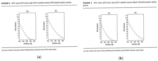
Figure 8.
(a) Dependence of on T (AECO Natural Gas Index (1 May 1998–30 April 1999)). (b) Dependence of on and T (AECO Natural Gas Index (1 May 1998–30 April 1999)). See Shahmoradi and Swishchuk (2016).
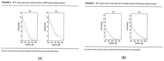
Figure 9.
(a) Dependence of the variance of on and T (AECO Natural Gas Index (1 May 1998–30 April 1999)). (b) Dependence of European call option price on maturity (months) ( and ) (AECO Natural Gas Index (1 May 1998–30 April 1999)). See Shahmoradi and Swishchuk (2016).
Figure 10.
Dependence of European call option price on maturity (months) ( and ) (AECO Natural Gas Index (1 May 1998–30 April 1999)). See Shahmoradi and Swishchuk (2016).
The volatility of crude oil prices is very important for policy makers, crude oil producers, and refineries. We used the most recent data starting from April 2016 from crude oil futures and options markets to model the dynamics of crude oil prices. Our results indicate that crude oil prices show significant jumps that are very frequent. Crude oil price returns show skew as well. These findings are consistent across all three models we used in this research.
In the case of JDM (see (8)), the volatility of size of the jumps is bigger than volatility of the diffusion part. The VG process (see (10)) results in slightly smaller volatility than JDM. The mean of the jump component size implied by JDM and the skew parameter of the VG process both indicate the existence of right-skew in crude oil price returns, but the NIG process (see (9)) implies that the density of returns are skewed to the left.
6. Energy Market Contracts with Delayed and Jumped Volatilities (Swishchuk 2020b)
We consider in this section stochastic modeling and pricing of energy markets’ contracts for stochastic volatilities with delays and jumps. Our model of stochastic volatility exhibits jumps and also past dependence: the behavior of a stock price right after a given time t not only depends on the situation at but also on the whole past (history) of the process up to time The spot price process is modeled by the OU process driven by independent increments process. The basic products in these markets are spot, futures, and forward contracts and options written on these. We study forwards and swaps. A numerical example is presented for stochastic volatility with delay using the Henry Hub daily natural gas data (1997–2011). Definition of IIP:(see Skorokhod 1991 and Benth et al. 2008a): An adapted RCLL stochastic process starting at zero is an IIP(independent Increment process) if it satisfies the following two conditions:
- The increments are independent r.v. for any partition and ;
- It is continuous in probability, that is, for every and :
If we add the condition that increments are stationary, then is called a Lévy process (see Sato 1999; Schoutens 2003).
Let the stochastic process be denoted as (we call it geometric models with stochastic delayed and jumped volatility):
where for
and for
where is the delay, and on the interval and where and are deterministic functions, , and
We remark that two factors, and (see (12) and (13)), represent the long- and short-term fluctuations of the spot dynamics, respectively, which may be correlated. We suppose that jumps components are independent, which is an obvious restriction of generality.
The deterministic seasonal price level is modeled by the function (seasonal function), which is assumed to be continuously differentiable. The coefficients are all continuous functions. We suppose that volatilities and are stochastic volatilities with delay and jumps. We consider two cases in this situation:
and
where and are two independent Brownian motions and and are two independent compensated Poisson processes with intensities and independent of and
We note that in Benth et al. (2008a), it was considered only deterministic and
Let the stochastic process be defined as (we call it arithmetic models with stochastic delayed and jumped volatility):
where and are defined for the geometric models above and the seasonality function is the same.
We suppose that for this model the volatilities and in (14) satisfied the same equations as for the case of the geometric models in (11)–(13).
We study the pricing of forwards and swaps for the above-mentioned model with delayed and jumped volatilities.
When entering the forward contract, one agrees on a future delivery time and the price to be paid for receiving the underlying. Suppose that the delivery time is with and that the agreed price to pay upon delivery is
which is the fundamental pricing relation between the spot and forward price. Since the energy markets are incomplete, the choice of martingale measure Q is open.
Let us consider swaps, using the electricity market as the typical example. The buyer of an electricity futures receives power during a settlement period (physically or financially), against paying a fixed price per MWh. Let be the electricity futures price at time t for the delivery period with
In general, we can write the link between a swap contract and the underlying spot as:
where w is a weight function.
The dynamics of forward price, wrt in the geometric model case is:
The risk-neutral dynamics of the swap price in the geometric models case is given by:
The risk-neutral dynamics of the swap price in the arithmetic models case is given by:
Numerical Example: Henry Hub Natural Gas Daily Spot Prices (1997–2011)
This numerical example and figures are borrowed from Otunuga and Ladde (2014). In this paper, the authors used the model for spot price with delayed stochastic volatility from the paper Kazmerchuk et al. (2005), and applied it to the Henry Hub daily natural gas dataset for the period 1 February 2001–30 September 2004. The data were collected from the United State Energy Information Administration website (www.eia.gov, accessed on 30 August 2020). From Figure 11 below, we can see the properties of the gas daily spot prices: randomly driven, non-negative, mean reversion, jumps (spikes), and unpredictable spot price volatility.
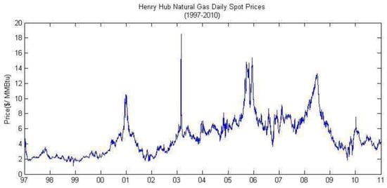
Figure 11.
Plot of Henry Hub Daily Natural Gas spot prices (1997–2011) (Otunuga and Ladde 2014).
Table 7 below gives descriptive statistics of Henry Hub Daily Natural Gas spot prices (1997–2011):
Table 7.
Descriptive statistics of Henry Hub Daily Natural Gas spot prices (1997–2011) (Otunuga and Ladde 2014).
As we can see from Table 7 above, the logarithmic price is better than the raw price data because the variance for log is the smallest.
A simple model for the spot price is considered:
where
and
The model for above is the same as the model for stochastic volatility with delay that we considered in Kazmerchuk et al. (2005).
A discrete scheme is implemented: where is the size of the mesh of the discrete-time grid and is the floor function. Descriptive statistics are in Table 7.
Estimated Parameters are in Table 8 (Otunuga and Ladde 2014):
Table 8.
Estimated parameters (Otunuga and Ladde 2014).
The graph below, Figure 12, includes the real, simulated spot prices and simulated expected spot price (Henry Hub Daily Natural Gas Dataset (1 February 2001–30 September 2004)):
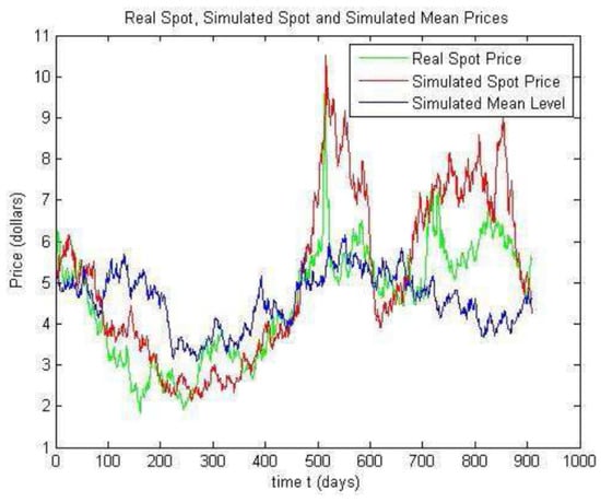
Figure 12.
Real, simulated spot prices and simulated expected spot price (Otunuga and Ladde 2014).
The graph below, Figure 13, shows the simulated from the Henry Hub Daily Natural Gas Dataset (1 February 2001–30 September 2004)).
Figure 13.
Simulated (Otunuga and Ladde 2014).
7. Mean-Reverting Processes in Alberta Energy Markets Modeling (Lu et al. 2021)
The paper Lu et al. (2021) is a bridge between fossil fuel energy research papers mentioned above (Swishchuk 2008, 2013b; Swishchuk and Cui 2013; Cui and Swishchuk 2015; Shahmoradi and Swishchuk 2016; Swishchuk 2020b) and clean energy research papers which will be produced in the near future.
In paper Lu et al. (2021), we:
- Introduced a fuel-switching price to the Alberta market, which is designed for encouraging power plant companies to switch from coal to natural gas when they produce electricity, which has been successfully applied to the European market;
- Considered an energy-switching price which considers power switch from natural gas to wind;
- Modeled these two prices using five mean reverting processes including a regime-switching processes, Lévy-driven Ornstein–Uhlenbeck process, and inhomogeneous geometric Brownian motion, and estimate them based on multiple procedures such as the maximum likelihood estimation and expectation–maximization algorithm;
- Proved previous results applied to the Albertan market, where the jump modeling technique is needed when modeling fuel-switching data;
- Explained the necessity of introducing regime-switching models to the fuel-switching data by showing that the regime-switching model is better fitted to the data.
Thus, we considered five mean-reverting processes in this paper:
- Inhomogeneous geometric Brownian motion (IGBM):where is a standard Brownian motion.
- OU process (OU):where is a standard Brownian motion.
- Lévy-driven OU process (LDOU):where is a Lévy process.
- Regime-switching OU process (RSOU)where is a continuous-time finite-state Markov chain, and is a bounded function of z.
- Regime-switching Lévy-driven OU process (RSLDOU):
After a comparison of models in (15)–(19), we were able to:
- (1)
- Conclude that the RSOU process and OU process are the best models for fuel-switching price and energy-switching price, respectively;
- (2)
- See that for the fuel-switching price, the regime-switching model largely increases the goodness of fit compared to other models, which indicates the important property of regime-switching for this price.
- (3)
- Conclude that jump modeling techniques are also important, as they increase the performance of the OU process, and this finding is similar to the previous results from North American and European markets.
The fuel-switching price in the Albertan market includes jumps and regime-switching, as reflected by the stochastic models. However, as the natural gas price keep decreasing in Alberta, more and more companies switched their power plant to natural gas, which is why we need to further consider energy-switching prices. The best fit of the OU process on energy-switching price reflects the steadiness of wind price, since it is a uniform distributed process.
8. Alternatives to Black-76 Model for Options Valuations of Futures Contracts (Swishchuk et al. 2021; Swishchuk 2020a)
In March 2020, the prompt month WTI futures contract settled below zero for the first time in the contract’s history. Many market participants apply the Black-76 model or some variation when calculating the value of the options on this futures contract as a relatively straightforward, parametric valuation method. However, Black 76 requires positive underlying market prices. The negative prompt month settlement price caused considerable consternation among energy traders and risk managers.
More generally, OTC options are also available on basis or differential prices. These transactions are options on the difference between two published indexes such as NYMEX Henry Hub and AECO (for natural gas) or Cushing WTI and Houston (for crude oil). As such, these instruments frequently have negative underlying market prices.
Thus, our task was to propose alternative models to Black-76 to valuate option prices when the underlying future contracts can assume negative values.
In Swishchuk et al. (2021), we proposed some alternatives to the Black-76 model to value European options on future contracts in which the underlying market prices can be negative or/and mean reverting. We specifically consider two models, namely Ornstein–Uhlenbeck (OU) for negative prices and continuous-time GARCH (or inhomogeneous geometric Brownian motion) for positive prices. We then analyze the results and compare them with Black-76, the most commonly used model, when the underlying market prices are positive. Numerical examples are presented using WTI and NYMEX NG datasets.
Our methodology is the following one:
- Take data (prices) and sketch their behavior, i.e., their evolution in time;
- If the prices are positive and not mean-reverting, then use the geometric Brownian motion (GBM) model for their evolution and Black-76 formula for option valuation of futures (see also formulas (BlCall) and (BlPut) in Swishchuk (2020a);
- If the prices are positive and mean-reverting, then use continuous-time GARCH (or, in other words, the inhomogeneous GBM model) model Swishchuk (2020a) and option pricing Formula (35) from Swishchuk (2008), Theorem 5.1;
- If the prices are both positive and negative, but not mean-reverting, then use the Bachelier model and their formula (see formulas (Ba_1) and (Ba_2) below and in Swishchuk (2020a);
- If the prices are both positive and negative, and mean-reverting with mean-reverting level then use the Ornstein–Uhlenbeck model and the formulas (OUCall_1) and (OUCall_2) below and from Swishchuk (2020a);
- If the prices are both positive and negative, and mean-reverting with mean-reverting level non-zero, then use Vasicek model and the formulas (VasCall_1) and (VasCall_2) below and from Swishchuk (2020a).
In this paper, we have shown how this methodology works on datasets presented by Scott Dalton (Ovintiv Services Inc.); namely, we used the WTI and NYMEX NG datasets.
Remark 2.
Bachelier (1900) was the first one who proposed to use Brownian motion as a model for stock price. He also presented the option Pricing formula. Good reference on stochastic modeling of electricity and related energy markets is Benth et al. (2008b). Black (1976) was the first to proposed to use the option pricing Black–Scholes approach (see Black and Scholes 1973) to option on futures pricing. An excellent reference on options, futures, and other derivatives is the book by Hull (1997).
9. A Vision to Transition to 100% Wind, Water, and Solar Energy in Canada (TheSolutionsProject 2023)
A group of U.S. civil engineering has calculated that Canada could be completely powered by renewable energy, if the country simply decides to do it. They say this would save billion CAD on health care costs every year and prevent 9884 annual air pollution deaths. Their research is available at TheSolutionsProject (2023).
2050 projected energy mix:
- –
- Onshore wind: ;
- –
- Offshore wind: ;
- –
- Hydroelectric: ;
- –
- Concentrated solar plants: ;
- –
- Commercial & government rooftop solar: ;
- –
- Solar plants: ;
- –
- Residential rooftop solar: ;
- –
- Wave devices: ;
- –
- Geothermal: ;
- –
- Tidal turbines: .
Figure 14 shows 2050 projected energy mix.
Figure 14.
2050 projected energy mix.
40-year jobs created (number of jobs where a person is employed for 40 consecutive years):
- –
- Construction jobs: 315,138
- –
- Operation jobs: 367,889
Figure 15 shows 40-year jobs created.
Figure 15.
40-year jobs created.
Reducing energy demand: (by improving energy efficiency and powering the grid with electricity from the wind, water, and sun, the overall energy demand is positively reduced).
Figure 16 shows reducing energy demand.
Figure 16.
Reducing energy demand.
Health cost savings:
- –
- Avoided health costs per year: B CAD (3.94% of the country’s GDP);
- –
- Lives lost to air pollution that could be saved each year: 9884.
Figure 17 shows health cost savings.
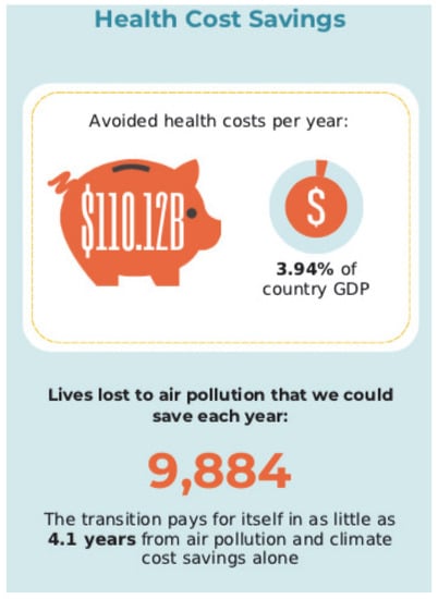
Figure 17.
Health cost savings.
Land usage (percentage of Canada land needed for all new wind, water, and solar generators):
- –
- Footprint Area:
- –
- Spacing Area:
Figure 18 shows land usage.
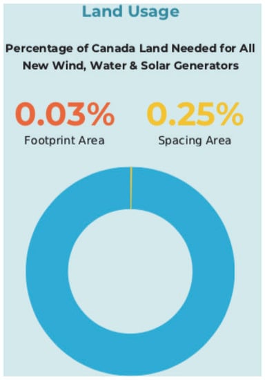
Figure 18.
Land usage.
Average energy costs in 2050:
- –
- Fossil Fuels & Nuclear Energy:
- –
- Wind, Water & Solar:
Figure 19 shows average energy costs in
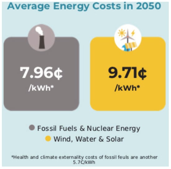
Figure 19.
Average energy costs in 2050.
Money in your pocket:
- –
- Energy cost savings per person: CAD;
- –
- Energy, health, and climate cost savings per person: CAD
Figure 20 shows money in your pocket.
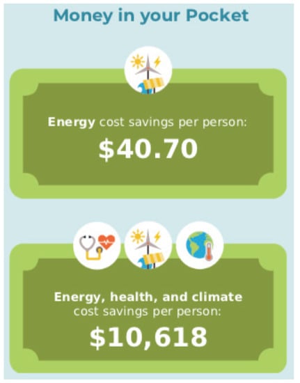
Figure 20.
Money in your pocket.
10. Wind and Solar Energy in Alberta (Dunn 2021)
Alberta could lead Canada in wind and solar power by 2025, experts say. It has been forecasted that of the combined utility-scale wind and solar capacity built in Canada over the next five years will be in Alberta. This would not include smaller renewable development such as residential rooftop solar.
According to the data that Rystad tracks, Alberta’s current renewable capacity includes 0.1 gigawatt (GW) of solar energy and 1.8 GW of wind energy. By 2025, this is expected to grow to 1.8 GW of solar energy and 6.5 GW of wind energy. Rystad forecasts Ontario will have about 1.8 GW solar energy and 5.8 GW wind energy in 2025. Tan said Alberta’s commitment to stop burning coal to generate electricity by 2030 “opens the door” for wind and solar energy to play a larger role.
We have 7693 solar PV systems in Alberta; residential, commercial, farm, other. Alberta now ranks third in Canada for installed wind energy capacity. Wind represents of Alberta’s total generation. Alberta’s hydro electric facilities represent of the market capacity of installed generation.
The travers solar project in Alberta is the size of 1600 football fields and is making Alberta a leader in green energy. Amazon announced in June 2021 that it will purchase power from a massive new solar farm in Alberta, marking the e-commerce giant’s second renewable energy investment in Canada.
Construction began in the fall of 2020 on Travers Solar, a 700-million CAD, 465-MW project southeast of Calgary, which its developers say will be the largest solar photovoltaic project in Canada and one of the largest in the world.
Privately held Greengate Power Corp. of Calgary has been working on the project for four years and is expected to have it completed by 2022. “It’ll consist of 1.3 million solar panels spread over more than 3000 acres (1215 hectares) of farmland”, said Dan Balaban, CEO of Greengate Power. “Furthermore, it’ll produce a sustainable source of energy for more than 150,000 homes”.
Remark 3.
Alberta is on track to meet its 2030 renewable energy goal ahead of schedule. An update for 2023 may be found ay https://thenarwhal.ca/alberta-renewable-energy-2030/ (accessed on 23 June 2023) (see Anderson 2022).
11. Energy Transition Center in Calgary, AB, Canada (Witzel 2022)
An investment of CAD was announced to support energy transition collaboration between the Calgary ecosystem and energy industry. The Energy Transition Centre (ETC) is a three-year project with a budget of 17.5 million. The Energy Transition Centre in downtown Calgary will support clean energy startup companies (see the Figure 21 and Figure 22).

Figure 21.
Ampersand building in downtown Calgary, site of the Energy Transition Centre.

Figure 22.
Gathering space at the Energy Transition Centre.
The University of Calgary ecosystem is poised to lead the energy transition with an investment announced this week from the Government of Canada. Prairies Economic Development Canada (PrairiesCan) is investing 2,140,205 CAD to support the Energy Transition Centre (ETC) in downtown Calgary.
The Energy Transition Centre is expected to support innovative clean energy development and generate economic activity through new business opportunities and research and development, while also assisting the commercialization of technologies for industry. Over the next three years, the initiative expects to create 25 new small- and medium-sized firms while assisting an additional 25 existing firms in accelerating their technologies for the clean technology sector. The ETC is a collaboration between the University of Calgary, Innovate Calgary, Avatar Innovations, and the energy industry. It is expected that programming at the ETC will engage highly qualified personnel from both the academic and industry sectors through career development, as well as technology development in areas of emerging technologies crucial for the energy transition. This includes engaging and supporting diverse industry employees as well as those involved in university research.
The ETC is designed to encourage energy transition solutions by providing programming that focuses on a mass upskilling of energy workers. This will be achieved through a training curriculum that cultivates cross-learning between energy professionals and university postdocs. Programs will also nurture transformative technologies through curriculum that entwines both business and technology de-risking components and provides access to technical experts and capital markets for commercialization.
12. Conclusions and Future Work
The paper provides an overview of our recent results of energy market modeling, including option pricing formula for a mean-reversion asset, variance and volatility swaps on energy markets, applications of weather derivatives on energy markets, pricing crude oil options using Levy processes, energy contracts modeling with delayed and jumped volatilities, applications of mean-reverting processes on Alberta energy markets, and alternatives to the Black-76 model for options valuation of futures contracts. We have also considered the clean renewable energy prospective in Canada, and, in particular in Alberta and Calgary.
Future research will be devoted to the renewable energy markets modeling, including wind, solar, and water energy modeling, weather derivatives modeling, and applications of Hawkes processes on energy markets.
13. Discussion
The paper reviews the author’s papers on energy markets modeling and many other related papers. More literature and archival contributions may be found in the referred papers (see References). Some relevant papers may also be found in https://www.mdpi.com/topics/energy_market_power_system (accessed on 23 June 2023) and in https://www.mdpi.com/1996-1073/13/16/4182 (accessed on 23 June 2023).
The main contributions of the paper consist of new models and results in modeling of energy markets prices and data, and the paper may be considered as a handbook in this area. The current paper/overview will help in modeling not only oil, gas, and electricity, but also in modeling renewable and clean energy data, e.g., Lu et al. (2021) shows how to model transition/switching from fossil energy to clean energy, e.g., from natural gas to wind. The future of this paper is promising; to name a few, weather derivatives will have an important application associated with climate change and alternatives to the Black-76 method and formula will have an application associated with negative prices, if it happens.
Funding
This research received no external funding.
Institutional Review Board Statement
Not applicable.
Informed Consent Statement
Not applicable.
Data Availability Statement
Not applicable.
Acknowledgments
The author thanks NSERC for continuing support.
Conflicts of Interest
The author declares no conflict of interest.
Abbreviations
The following abbreviations are used in this manuscript:
| MDPI | Multidisciplinary Digital Publishing Institute |
| DOAJ | Directory of open access journals |
| TLA | Three-letter acronym |
| LD | Linear dichroism |
References
- Anderson, Drew. 2022. The Narwhal: Guess What? Alberta Is on Track to Meet Its 2030 Renewable Energy Goal Ahead of Schedule. December. Available online: https://thenarwhal.ca/alberta-renewable-energy-2030/ (accessed on 23 May 2023).
- Askari, Hossein, and Noureddine Krichene. 2008. Oil Price Dynamics. Energy Economics 30: 2134–53. [Google Scholar] [CrossRef]
- Bachelier, L. 1900. Theorie de la Speculation. Ph.D. thesis, Sorbonne University, Paris, France. [Google Scholar]
- Benth, Fred Espen, and Jūratė Šaltytė-Benth. 2005. Stochastic Modelling of Temperature Variations with a View Towards Weather Derivatives. Applied Mathematical Finance 12: 53–85. [Google Scholar] [CrossRef]
- Benth, Fred Espen, Jūratė Šaltytė Benth, and Steen Koekebakker. 2008a. Stochastic Modelling of Electricity and Related Markets. Singapore: World Scientific. [Google Scholar]
- Benth, Fred Espen, Jūratė Šaltytė Benth, and Steen Koekebakker. 2008b. Stochastic Modelling of Electricity and Related Markets. Number 11 in Advanced Series on Statistical Science & Applied Probability. Singapore: World Scientific. [Google Scholar]
- Black, Fischer. 1976. The pricing of commodity contracts. Journal of Financial Economics 3: 167–79. [Google Scholar] [CrossRef]
- Black, Fischer, and Myron Scholes. 1973. The Pricing of Options and Corporate Liabilities. The Journal of Political Economy 81: 637–57. [Google Scholar]
- Borowski, Piotr F. 2020. Zonal and Nodal Models of Energy Market in European Union. Energies 13: 4182. [Google Scholar] [CrossRef]
- Bos, Len, Antony Ware, and Boris Pavlov. 2002. On a semi-spectral method for pricing an option on a mean-reverting asset. Quantitative Finance 2: 337–45. [Google Scholar] [CrossRef]
- Broadie, Mark, and Ashish Jain. 2008. Pricing and Hedging Volatility Derivatives. The Journal of Derivatives 15: 7–24. [Google Scholar] [CrossRef]
- Brockhaus, Oliver, and Douglas Long. 2000. Volatility swaps made simple. Risk-London Magazine Limited 13: 92–95. [Google Scholar]
- Carr, Peter, and Dilip Madan. 1998. Towards a Theory of Volatility Trading. In Volatility: New Estimation Techniques for Pricing Derivatives, 7th ed. Edited by Robert A. Jarrow. London: Risk Books. [Google Scholar]
- Considine, Geoffrey. 2000. Introduction to Weather Derivaties. Aquila Energy, 1–10. [Google Scholar]
- Crosby, John. 2008. A multi-factor jump-diffusion model for commodities. Quantitative Finance 8: 181–200. [Google Scholar] [CrossRef]
- Cui, Kaijie, and Anatoliy Swishchuk. 2015. Applications of weather derivatives in the energy market. The Journal of Energy Markets 8: 59–76. [Google Scholar] [CrossRef]
- De Brito, Marcelle Caroline Thimotheo, Amaro O. Pereira Junior, Mario Veiga Ferraz Pereira, Julio César Cahuano Simba, and Sergio Granville. 2022. Competitive Behavior of Hydroelectric Power Plants under Uncertainty in Spot Market. Energies 15: 7336. [Google Scholar] [CrossRef]
- Diewvilai, Radhanon, and Kulyos Audomvongseree. 2022. Possible Pathways toward Carbon Neutrality in Thailand’s Electricity Sector by 2050 through the Introduction of H2 Blending in Natural Gas and Solar PV with BESS. Energies 15: 3979. [Google Scholar] [CrossRef]
- Dornier, Fred, and Mark Queruel. 2000. Caution to the Wind. Energy and Power Risk Management 13: 30–32. [Google Scholar]
- Dunn, Carolyn. 2021. CBC News: How Canada’s Largest Solar Farm is Changing Alberta’s Landscape. November. Available online: https://www.cbc.ca/news/canada/calgary/travers-solar-project-vulcan-1.6233629 (accessed on 23 May 2023).
- Ellen, Jovin. 1998. Advances on the Weather Front (An Overview of the U.S. Weather Derivatives Market, Global Energy Risk). Electrical World 212: S6. [Google Scholar]
- Hamisultane, Hélène. 2006. Extracting Information from the Market to Price the Weather Derivatives. Available online: https://shs.hal.science/halshs-00079192/document (accessed on 23 June 2023).
- Hull, John C. 1997. Option, Futures, and Other Derivatives. Hoboken: Prentice Hall. [Google Scholar]
- Ikeda, Nobuyuki, and Shinzo Watanabe. 1981. Stochastic Differential Equations and Diffusion Processes. Tokyo: Kodansha Ltd. [Google Scholar]
- Ismail, Firas B., Maisarah Mazwan, Hussein Al-Faiz, Marayati Marsadek, Hasril Hasini, Ammar Al-Bazi, and Young Zaidey Yang Ghazali. 2022. An Offline and Online Approach to the OLTC Condition Monitoring: A Review. Energies 15: 6435. [Google Scholar] [CrossRef]
- Kaminski, Vincent. 1998. Pricing Weather Derivatives (Global Energy Risk). Electrical World 212: S6. [Google Scholar]
- Kazmerchuk, Yuriy, Anatoliy Swishchuk, and Jianhong Wu. 2005. A Continuous-time GARCH model for stochastic volatility with delay. The Canadian Applied Mathematics Quarterly 13: 123–49. [Google Scholar]
- Lu, Weiliang, Alexis Arrigoni, Anatoliy Swishchuk, and Stéphane Goutte. 2021. Modelling of Fuel- and Energy-Switching Prices by Mean-Reverting Processes and Their Applications to Alberta Energy Markets. Mathematics 9: 709. [Google Scholar] [CrossRef]
- Madan, Dilip, and Eugene Seneta. 1990. The Variance Gamma (V.G.) Model for Share Market Returns. The Journal of Business 63: 511–24. [Google Scholar] [CrossRef]
- Mallala, Balasubbareddy, Venkata Prasad Papana, Ravindra Sangu, Kowstubha Palle, and Venkata Krishna Reddy Chinthalacheruvu. 2022. Multi-Objective Optimal Power Flow Solution Using a Non-Dominated Sorting Hybrid Fruit Fly-Based Artificial Bee Colony. Energies 15: 4063. [Google Scholar] [CrossRef]
- Merton, Robert C. 1976. Option pricing when underlying stock returns are discontinuous. Journal of Financial Economics 3: 125–44. [Google Scholar] [CrossRef]
- Navarro, Ramon, H. Rojas, Izabelly S. De Oliveira, J. E. Luyo, and Y. P. Molina. 2022. Optimization Model for the Integration of the Electric System and Gas Network: Peruvian Case. Energies 15: 3847. [Google Scholar] [CrossRef]
- Otunuga, Olusegun Michael, and Gangaram S. Ladde. 2014. Stochastic Modeling of Energy Commodity Spot Price Processes with Delay in Volatility. American International Journal of Contemporary Research 4: 1–19. [Google Scholar]
- Pilipović, Dragana. 1998. Energy Risk: Valuing and Managing Energy Derivatives. New York: McGraw-Hill. [Google Scholar]
- Podkovalnikov, Sergei, Lyudmila Chudinova, Ivan L. Trofimov, and Leonid Trofimov. 2022. Structural and Operating Features of the Creation of an Interstate Electric Power Interconnection in North-East Asia with Large-Scale Penetration of Renewables. Energies 15: 3647. [Google Scholar] [CrossRef]
- Sato, Ken-iti. 1999. Lévy Processes and Infinitely Divisible Distributions. Number 68 in Cambridge Studies in Advanced Mathematics. Cambridge and New York: Cambridge University Press. [Google Scholar]
- Schoutens, Wim. 2003. Lévy Processes in Finance: Pricing Financial Derivatives. Wiley Series in Probability and Statistics; Chichester, West Sussex and New York: J. Wiley. [Google Scholar]
- Schwartz, Eduardo S. 1997. The Stochastic Behavior of Commodity Prices: Implications for Valuation and Hedging. The Journal of Finance 52: 923–73. [Google Scholar] [CrossRef]
- Shahmoradi, Akbar, and Anatoliy Swishchuk. 2016. Pricing crude oil options using Lévy processes. The Journal of Energy Markets 9: 47–63. [Google Scholar] [CrossRef]
- Shobeiri, Elaheh, Huan Shen, Filippo Genco, and Akira Tokuhiro. 2022. Investigating Long-Term Commitments to Replace Electricity Generation with SMRs and Estimates of Climate Change Impact Costs Using a Modified VENSIM Dynamic Integrated Climate Economy (DICE) Model. Energies 15: 3613. [Google Scholar] [CrossRef]
- Skorokhod, Anatoliĭ Vladimirovich. 1991. Random Processes with Independent Increment. Dordrecht: Springer Science+Business Media. [Google Scholar]
- Sun, Bo, Siyuan Cheng, Jingdong Xie, and Xin Sun. 2022. Identification of Generators’ Economic Withholding Behavior Based on a SCAD-Logit Model in Electricity Spot Market. Energies 15: 4135. [Google Scholar] [CrossRef]
- Swishchuk, Anatoliy. 2008. Explicit Option Pricing Formula for a Mean-Reverting Asset in Energy Market. Journal of Numerical and Applied Mathematics 1: 216–33. [Google Scholar]
- Swishchuk, Anatoliy. 2013a. Modeling and Pricing of Swaps for Financial and Energy Markets with Stochastic Volatilities. Singapore: World Scientific. [Google Scholar] [CrossRef]
- Swishchuk, Anatoliy. 2013b. Variance and volatility swaps in energy markets. The Journal of Energy Markets 6: 33–49. [Google Scholar] [CrossRef]
- Swishchuk, Anatoliy. 2020a. Alternatives to Black-76 Model for Options Valuation of Futures Contracts (Lectures’ Notes). Unpublished manuscript. [Google Scholar] [CrossRef]
- Swishchuk, Anatoliy. 2020b. Stochastic Modeling and Pricing of Energy Markets’ Contracts with Local Stochastic Delayed and Jumped Volatilities. In Handbook of Energy Finance: Theories, Practices and Simulations. Edited by Stéphane Goutte and Duc Khuong Nguyen. Singapore: World Scientific Publishing Co. Pte. Ltd., pp. 247–66. [Google Scholar]
- Swishchuk, Anatoliy, Ana Roldan-Contreras, Elham Soufiani, Guillermo Martinez, Mohsen Selfi, Nishant Agrawal, and Yao Yao. 2021. Alternatives to Black-76 Model for Options Valuations of Futures Contracts. Wilmott 2021: 40–49. [Google Scholar] [CrossRef]
- Swishchuk, Anatoliy, and Kaijie Cui. 2013. Weather Derivatives with Applications to Canadian Data. Journal of Mathematical Finance 3: 81–95. [Google Scholar] [CrossRef]
- TheSolutionsProject. 2023. Available online: https://thesolutionsproject.org/ (accessed on 23 May 2023).
- Ullah, Zahid, Arshad, and Hany Hassanin. 2022. Modeling, Optimization, and Analysis of a Virtual Power Plant Demand Response Mechanism for the Internal Electricity Market Considering the Uncertainty of Renewable Energy Sources. Energies 15: 5296. [Google Scholar] [CrossRef]
- Wang, Jidong, Jiahui Wu, and Yingchen Shi. 2022. A Novel Energy Management Optimization Method for Commercial Users Based on Hybrid Simulation of Electricity Market Bidding. Energies 15: 4207. [Google Scholar] [CrossRef]
- Witzel, Jordan. 2022. University of Calgary: $2.14M Investment Announced to Support Energy Transition Collaboration between UCalgary Ecosystem and Energy Industry. January. Available online: https://ucalgary.ca/news/214m-investment-announced-support-energy-transition-collaboration-between-ucalgary-ecosystem-and (accessed on 23 May 2023).
- Yor, Marc. 1992. On some exponential functionals of Brownian motion. Advances in Applied Probability 24: 509–31. [Google Scholar] [CrossRef]
- Yor, Marc, and Hiroyuki Matsumoto. 2005. Exponential functionals of Brownian motion, I: Probability laws at fixed time. Probability Surveys 2: 312–47. [Google Scholar] [CrossRef]
- Zhang, Bidan, Yang Du, Xiaoyang Chen, Eng Gee Lim, Lin Jiang, and Ke Yan. 2022. Potential Benefits for Residential Building with Photovoltaic Battery System Participation in Peer-to-Peer Energy Trading. Energies 15: 3913. [Google Scholar] [CrossRef]
- Zhao, Jun, Xiaonan Wang, and Jinsheng Chu. 2022. The Strategies for Increasing Grid-Integrated Share of Renewable Energy with Energy Storage and Existing Coal Fired Power Generation in China. Energies 15: 4699. [Google Scholar] [CrossRef]


Disclaimer/Publisher’s Note: The statements, opinions and data contained in all publications are solely those of the individual author(s) and contributor(s) and not of MDPI and/or the editor(s). MDPI and/or the editor(s) disclaim responsibility for any injury to people or property resulting from any ideas, methods, instructions or products referred to in the content. |
© 2023 by the author. Licensee MDPI, Basel, Switzerland. This article is an open access article distributed under the terms and conditions of the Creative Commons Attribution (CC BY) license (https://creativecommons.org/licenses/by/4.0/).