Abstract
In this paper, we study a risk model with stochastic premium income and its impact on solvency risk management. It is assumed that both the premium arrival process and the claim arrival process are modelled by homogeneous Poisson processes, and that the premium amounts are modelled by independent and identically distributed random variables. While this model has been studied in the existing literature and certain explicit results are known under more restrictive assumptions, these results are relatively difficult to apply in practice. In this paper, we investigate the factors that differentiate this model and the classical risk model. After reviewing various known results of this model, we derive a simulation approach for obtaining the probability of ultimate ruin based on importance sampling, which does not require specific distributions for the premium and the claim. We demonstrate this approach first with examples where the distribution of the sampling random variable can be identified. We then provide additional examples where we use the fast Fourier transform to obtain an approximation of the sampling random variable. The simulated results are compared with the known results for the probability of ruin. Using the simulation approach, we apply this model to a real-life auto-insurance data set. Differences with the classical model are then discussed. Finally, we comment on the suitability and impact of using this model in the context of solvency risk management.
1. Introduction
The studies of an insurer’s cashflow date back to the early 1900s. To model the cashflow of an insurer, it suffices to consider the premium income and the claim payments arriving over time. In the most basic setting, investing is not considered, the rate at which the insurer collects premiums is assumed to be constant, and the claim arrivals are modelled by a homogeneous Poisson process. This model is known as the classical risk model or the compound-Poisson risk model. Under this model, the surplus process of an insurer is given by
where is the initial surplus of the insurer, is the continuous premium rate, is a homogeneous Poisson process that counts the number of claim arrivals up to time t, and is the amount of the kth claim. The mathematical properties of a homogeneous Poisson process make the analysis of this model tractable. Consequently, many theoretical results under this model have been obtained through probabilistic arguments. An important advancement in this field was made by Gerber and Shiu (1998), where the analysis of various quantities of interest, such as the probability of ultimate or finite-time ruin, the Laplace transform of the time of ruin, the distribution of the deficit at ruin, etc., are captured in a systematic way by the discounted penalty function, also known as the Gerber–Shiu function,
where is the random time of ruin, the penalty function, w, is a bi-variate function of the surplus just before ruin and the deficit at ruin, and is the discount factor. By setting different values of w and , the Gerber–Shiu function reduces to various quantities of interest. See, for example, Asmussen and Albrecher (2010), Chapter XII for a summary.
The classical risk model (1) is mathematically convenient as it is tractable, but its restrictive assumptions limit its applicability to real-world insurance portfolios. To address this, researchers have introduced various stochastic processes to enhance the model’s accuracy. An early attempt was Andersen (1957), where the author replaced the homogeneous Poisson process by a renewal process, allowing for arbitrary inter-arrival time distributions and providing more flexibility than the exponential inter-arrival times of the Poisson process. However, renewal processes still cannot capture time inhomogeneity observed in claim arrivals.
To model time-dependent behaviours, stochastic processes incorporating periodicity and non-stationarity have been considered. Asmussen and Rolski (1994) introduced a risk model with a periodic claim arrival process to capture seasonal fluctuations, Morales (2004) demonstrated simulation methods for calculating ruin probabilities in this context, and Miao et al. (2023a) considered a risk model where both premiums and claims exhibit seasonalities. More recently, Cox processes, where the claim arrival intensity itself is stochastic, have gained attention. Notable examples include the shot-noise Cox process, studied by Dassios and Jang (2003), Albrecher and Asmussen (2006), Dassios et al. (2015), and Avanzi et al. (2021b), which models sudden surges in claim rates due to external events. The Markov-modulated Poisson process (e.g., Asmussen (1989); Lu and Li (2005); Avanzi et al. (2021a)) allows the model to switch between different regimes with distinct claim arrival rates. A non-stationary Cox process incorporating trends and cycles over time was considered in Albrecher et al. (2021). These stochastic processes enhance claim modelling by capturing complex patterns like time inhomogeneity, regime switching, and external shocks.
Modifications have also been proposed for premium income by replacing deterministic premium income with a stochastic premium process. This accounts for uncertainties due to economic conditions or policyholder behaviour. This stochastic premium model remains mathematically tractable and has been studied extensively. Boikov (2003) derived integral equations for ultimate and finite-time survival probabilities under this model, providing closed-form expressions in special cases. Labbé and Sendova (2009) explored the expected discounted penalty function, establishing renewal and integral equations. Albrecher et al. (2010) offered alternative derivations using exponential claim sizes before generalising to arbitrary distributions. Additionally, Vidmar (2018) investigated models with stochastic dependence between premiums and claim arrivals, reflecting scenarios where economic factors simultaneously influence both income and outflows.
While the stochastic premium model is not new and a great deal of risk theory results are known, the existing results are often from a theoretical point of view. Moreover, the results are mostly given in a non-explicit form, often involving integral equations and Laplace transforms. These results, while providing mathematical insights into the model, are relatively hard to implement in practice. Explicit results may be obtained by imposing assumptions on the distributions of premiums and claims, such as the examples in Labbé and Sendova (2009). However, these assumptions are often quite restrictive and may not be suitable for real-life situations. Another approach is to explore numerical approximations for specific quantities. Temnov (2004) derived an expression for the probability of ruin and developed a numerical approximation procedure based on Fourier transforms. This approach does not impose assumptions on premiums and claims, and hence may be applied to more general cases. The convolution formula for the probability of ruin has the same form as the classical model and is given by
where and is the kth fold self-convolution of a cumulative distribution function, . Although this formula is succinct and works for all distributions, neither the value of q nor are known. Both of these quantities need to be evaluated numerically through a chain of approximations. Multiple steps of truncation are also involved in the process. These steps increase the complexity of the computations and introduce the potential for accumulated numerical errors.
In this paper, we aim to investigate the impact of applying this model in practice in the solvency risk management context. We first present a simulation-based method to obtain the probability of ultimate ruin. As discussed in Asmussen and Binswanger (1997), this is a rare event simulation with an infinite time horizon. A common technique to solve this issue is applying Esscher transforms to the sample random variables. This technique finds many applications in finance and insurance; see, for example, Bühlmann et al. (1998); Elliott et al. (2005); and Chuang and Brockett (2014). Taking advantage of the fact that the drop of surplus upon each claim arrival follows a compound-geometric distribution, we derive a simulator based on Esscher transforms. The simulation approach does not require specific distributions for premiums and claims and can be applied to a wide range of real-life scenarios. In comparison with the numerical approximation approach, the simulation approach does not require one to evaluate the probability of ruin for all admissible values of the initial surplus. It also involves fewer steps and truncations. Using the simulation approach, we first give two examples with simple distributions where the exact distribution of the sampling random variable can be identified. We then present a Fourier transform-based algorithm to deal with more general cases with other distributions. The simulated results are compared with known explicit results to highlight the differences from the classical model. We then investigate whether applying this model in practice requires significantly different resources to manage solvency risk. To this end, we fit the model to a real-life auto-insurance data set. We compare this model with the classical model. We discover that the classical model is a good approximation to the stochastic premium model under certain circumstances. However, the differences between the two models could be more significant for other lines of insurances. Moreover, the changing physical environment may deteriorate the claim experience for an established pool of policies. One such example is the significantly increased claims related to extreme weather events from catastrophic insurances over the past few years. As we show using a modified and hypothetical version of the data set, simply increasing the premium amount to counter the increased claims is not sufficient from a solvency risk management point of view. These results indicate that the stochastic premium model has practical value, and that the differences from the classical model vary depending on the characteristics of the specific insurance product that is studied.
This paper is structured as follows. Some useful mathematical tools and their properties are reviewed in Section 2. In Section 3, we introduce formally the risk model with stochastic premium income and briefly summarise known results in the existing literature. A simulator based on importance sampling is derived in Section 4. An approximation method based on the fast Fourier transform is also presented in this section. Examples are given to illustrate the simulation approach. In Section 5, we apply the stochastic premium model to a real-life auto-insurance data set and comment on the differences it makes. We then compare the performance of the model under different scenarios using modified and hypothetical versions of the auto-insurance data set. We comment on the application of the model in a changing environment and its impacts. Conclusions are given in Section 6.
2. Preliminaries
In this section, we present some useful mathematical results that will be used later in the paper.
2.1. Moment Generating Function and Cumulant Generating Function
One convenient way to represent a random variable is through its generating functions. Let X be a random variable. Its moment generating function (m.g.f.), , and its cumulant generating function (c.g.f.), , are defined by
These two functions are not defined for all distributions. For example, they are not defined for the Cauchy distribution. Notice that it is possible that the expectation (2) converges to infinity for some , i.e., the generating functions are only defined on a subset of . We thus require the following definition.
Definition 1.
The domain of a function, f, denoted by , is the subset of , where the value of the function is finite, i.e.,
Moment generating functions and cumulant generating functions are convenient because they provide a systematic way to calculate the moments of a random variable. If there exists , such that , then we have the following convenient results
2.2. Importance Sampling and Esscher Transform
Importance sampling is an important simulation technique. It is often used to achieve variance reduction in rare event simulations.
Definition 2
(Importance sampling). Suppose X is a -valued random variable defined on the measurable space . Let and be two measures on the same measurable space. Let be a measurable function. Then we have
where is the Radon–Nikodym derivative and is called the likelihood ratio.
If the random variable in Definition 2 has a probability density function (p.d.f.) f under measure and has a p.d.f. g under measure , then the likelihood ratio is , i.e., Equation (4) becomes
where has the p.d.f. g.
A major benefit of importance sampling is variance reduction. Namely, suppose we are interested in estimating by simulation. We may simulate X under the probability measure , calculate , repeat this procedure n times and calculate the average of these n different realisations. To reduce the variance of the estimator, we simply increase the number of simulations, n. This approach is called the crude Monte Carlo method or the naïve Monte Carlo method. Under certain circumstances, this method is not efficient. These situations usually involve simulating some rare events associated with very small probabilities. A number of variance-reduction techniques exist for rare event simulation, see Bucklew (2013) for more details. When using importance sampling, we simulate X under the probability measure . The new estimator is . We may choose an appropriate such that the variance of the estimator is smaller than that of the crude estimator.
The key to importance sampling is to specify a new probability measure under which the random variable X has an appropriate distribution. If the original distribution is absolutely continuous, i.e., the p.d.f. exists, then it suffices to specify the new p.d.f. under the new measure. The importance sampling for this case is given by Equation (5). We introduce next a method to define a new probability measure.
Definition 3
(Esscher transform). Let X be a -valued random variable defined on a measure space . Suppose X has the m.g.f. and the c.g.f. . The Esscher transform of the measure , denoted by , is given by the likelihood ratio
where θ is the parameter of the Esscher transform.
In this paper, we denote random variables related to an Esscher-transformed measure by a tilde together with the transformation parameter given in a pair of parentheses. It is easy to show that the m.g.f. of the transformed distribution, denoted by , is
Furthermore, if a random variable, X, has a p.d.f. then the p.d.f. of the transformed distribution, denoted by , is given by
Some common distributions are invariant under the Esscher transform. For example, if X is exponentially distributed with parameter , then its Esscher transform with parameter is also an exponential distribution with parameter . If X is geometrically distributed with parameter p, then its Esscher transform with parameter also follows a geometric distribution with parameter . For more details on the Esscher transform and its applications, see, for example, Asmussen and Glynn (2007).
If the likelihood ratio of the importance sampling is defined by Equation (6), then we have
By Equations (3) and (8), we have
Equation (9) establishes a relationship between the expected value under the new probability measure and the c.g.f. under the original probability measure. This relationship is utilised to derive the estimator of the probability of ultimate ruin in Section 4.
Lemma 1 extends Equation (8) to a random number of random variables.
Lemma 1.
Let be independent and identically distributed random variables with a common c.g.f., Γ, then
2.3. Fourier Transform and Fast Fourier Transform
The Fourier transform is a useful tool that is used extensively in science and engineering. It studies how a function may be approximated by a sum of trigonometric functions.
Definition 4
(Fourier transform). Let be an integrable function, the Fourier transform of f, denoted by , is given by
where . The inverse Fourier transform of a function g, denoted by , is defined by
Remark 1.
There are different definitions of the Fourier transform and its inverse. Generically, the Fourier transform can be defined as
where A and B are two constants. For possible combinations of these two constants and their properties, see Osgood (2019), Chapter 2.4. We choose because under this definition the Fourier transform of a probability function is the characteristic function of the distribution.
The discrete Fourier transform is utilised in many practical applications. Suppose instead of a continuous function, f, we have equally spaced samples, i.e.,
where for all , .
Definition 5
(Discrete Fourier transform). For a finite sequence , the discrete Fourier transform and its inverse are defined as
The discrete Fourier transform, which operates on a finite discrete sequence, may be viewed as a discretisation of a Fourier transform, which operates on a continuous integrable function. As the number of samples increases, the discrete Fourier transform converges to the Fourier transform. The discrete Fourier transform is of great practical value because it can be implemented through a highly efficient algorithm, called the fast Fourier transform. A direct implementation of the discrete Fourier transform has a computational complexity of , while an implementation using the fast Fourier transform has a computational complexity of . For more details, see, for example, Cooley and Tukey (1965); Brigham (1988); and Osgood (2019), Chapter 7.
In risk theory, Fourier transforms are often used to evaluate the probability function of a compound distribution of the form , where N is a non-negative integer-valued random variable, and s are independent and identically distributed positive random variables. To obtain the exact density function or mass function of the compound distribution, one needs to evaluate the self-convolution of , which is often cumbersome if possible at all. Some approximation methods exist. Examples of these approximations include normal approximation, gamma approximation, and Esscher approximation. For a review on this topic, see Hardy (2006). Under certain conditions, exact numerical methods also exist, notably the Panjer recursion, see Klugman et al. (2012), Chapter 9.6; and Sundt and Jewell (1981).
Using the discrete Fourier transform, one may obtain an approximation of the probability mass function of the compound distribution . We assume that the compounded random variable has mass at equally spaced points with probabilities , respectively. Notice that we assume that the support of the distribution is discrete. If the distribution of the compounded random variable is continuous, then it is discretised first. Under this assumption, the compound random variable is discrete. For all , denote
Let and be the kth expression of the discrete Fourier transform of the sequences and , respectively. These two sequences are approximations of the characteristic functions of and S. To obtain an approximation of the probability mass function of S, one first obtains the sequence , then calculates
where is the probability generating function (p.g.f.) of N. Finally, the mass function of S is
For more details of this algorithm, see, for example, Albrecher et al. (2017), Chapter 6.4; and Asmussen and Glynn (2007), Chapter 2e. We also note that this algorithm yields an approximation of the actual mass probability. The error introduced by the approximation is studied in Grübel and Hermesmeier (1999), where a procedure to reduce the approximation error is also presented.
3. A Risk Model with Stochastic Premium Income
One way to extend the classical model (1) is to replace the deterministic premium income by a stochastic process. The surplus process is defined by
where is the initial surplus, the premium counting process is a homogeneous Poisson process with rate , the claim counting process, , is a homogeneous Poisson process with rate , is the amount of the kth premium arrival, and is the size of the kth claim arrival. We assume that , , s, and s are mutually independent. We make the following assumptions on the surplus process.
Assumption 1.
The relative security loading is positive, i.e., .
Assumption 2.
The m.g.f. of and , denoted by and , respectively, exist. Furthermore, for all , there is a and a , such that and .
Since the classical model has been thoroughly studied, it often serves as the benchmark model for comparison. We are interested in how much additional risk the stochastic premium model (10) can capture compared with the classical model (1). To this end, we need to change only the premium process of these two models while holding other factors unchanged.
Definition 6
(Comparable risk models). Two risk models of the general form
where , which is the total premium amount collected up to time t, and , which is the total claim amount paid up to time t, are comparable if and for all .
The classical model (1) and the stochastic premium model (10) are comparable if , while N and s are the same in these two models.
Some ruin theory results have been derived for the stochastic premium model using both probabilistic arguments and through the Gerber–Shiu function. The next theorem is a collection of known results pertinent to the contents of this paper.
Theorem 1.
For the stochastic premium model (10), define the time of ruin
The probability of ruin is Let be the survival probability. Then
- (Boikov 2003) The survival probability satisfieswhere F is the cumulative distribution function of the claim size random variable , and G is the cumulative distribution function of the premium amount random variable .
- (Boikov 2003) Let be a positive root ofthen by a martingale argument we have
- (Temnov 2004) Let be the probability of ruin under the classical model (1) with , then for all .
- (Temnov 2004) The classical model may be expressed as a limiting case of the stochastic premium model. The ruin probability satisfiesfor all
For the proof of these results, the reader is referred to the original papers.
4. A Simulation Approach
In this section, we derive a simulation approach to obtain the probability of ruin. We first obtain an expression of the probability of ruin using a change-of-measure argument. The derivation is similar to Pham (2007); Asmussen and Albrecher (2010); and Grandell (2012).
In the classical model, the surplus increases linearly between two claims and drops at the arrival of a claim. In the stochastic premium model, the surplus has an upward jump at the arrival of a premium and has a downward drop at the arrival of a claim. Figure 1 gives a sample trajectory of the surplus process under the stochastic premium model.
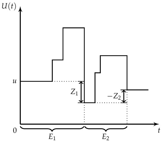
Figure 1.
A sample trajectory of the surplus process.
Let be the time between the st claim arrival and the kth claim arrival. (Given the Poisson nature of claim arrivals, we may assume that the 0th arrival is at 0 without loss of generality.) Since is a homogeneous Poisson process with rate , we know that s are independent and identically distributed exponential random variables with parameter . Let be the kth drop in the surplus process, i.e.,
where is the number of premium arrivals between the st claim and the kth claim, which may be expressed as
Since the premium arrival process, H, is a homogeneous Poisson process with intensity , we know that follows a Poisson distribution, given ,
Using the m.g.f., it is easy to prove the following result.
Lemma 2.
is geometrically distributed with probability of success .
Proof.
The m.g.f. of , denoted by , may be obtained by using the law of total expectation,
Expression (13) is the m.g.f. of a geometric distribution with probability of success . By the uniqueness of the m.g.f., we establish the result. □
Lemma 2 indicates that the total premium amount between the two claim arrivals in Equation (12) has a compound geometric distribution. This property is convenient since a number of methods exist for estimating the p.d.f. of this compound distribution.
As in the classical model, ruin can only happen when there is a claim arrival. Consequently, it suffices to consider the embedded discrete-time surplus process defined at each claim arrival, namely,
where is the surplus at the nth claim arrival and is the drop of surplus defined in Equation (12). The discrete time of ruin, defined as the number of claim arrivals at time of ruin, is then
A Lundberg-type upper bound for the probability of ruin is given in Theorem 2.
Theorem 2.
Suppose that a stochastic premium model satisfies Assumptions 1 and 2. Then the probability of ultimate ruin satisfies
where is the positive root of the equation
where and are the c.g.f. of and , respectively, is the p.g.f. of , and is the m.g.f. of .
Proof.
We first prove that Equation (16) has a root in . Assumption 1 indicates that
By definition, the c.g.f. satisfies
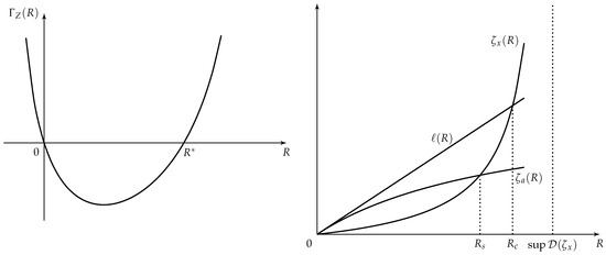
and therefore, there exists , such that . By Assumption 2, goes to infinity when R approaches the endpoint of its domain. Consequently, there exists , such that . By the continuity of , we may conclude that there exists a positive root to Equation (16) in the interval . Figure 2 gives an illustration of Equation (16). By the convexity of the c.g.f., it is easy to show that
Figure 2.
(Left): an example of Equation (16); (right): a comparison of adjustment coefficients under the classical model and under the stochastic premium model.
Consider a new probability measure defined by an Esscher transform with parameter . By Equation (9), we have
i.e., the random walk, , in Equation (15) has a positive drift after the Esscher transform and, consequently, for any positive u, the event is certain. By Lemma 1, and observing that the time of ruin, , is a stopping time with respect to the -algebra generated by , the probability of ultimate ruin under the original probability measure, , may be expressed as
By the definition of the time of ruin (15), we know that
and substituting the summation in Equation (18) by u, we have
□
Remark 2.
Corollary 1.
The upper bound in Theorem 2 is greater than or equal to the Lundberg upper bound for the comparable classical model.
Proof.
It suffices to show that the adjustment coefficient of the stochastic premium model is smaller than or equal to the adjustment coefficient of the comparable classical model. We first prove the existence of the roots. The Lundberg equations, expressed in terms of moment generating functions, for the classical model (1) and the comparable stochastic premium model (10) are given by
For notational convenience, denote by
and observe that is an increasing, continuous and convex function, ℓ is an increasing, continuous and linear function, and is an increasing, continuous and concave function, which are demonstrated by their respective derivatives
We have further
meaning that 0 is a root to both Equation (19) and Equation (20), and that there exists a sufficiently small , such that, for all , and . Equation (21) also implies that for all . Consider Equation (20), we have
Since is monotonically increasing, we have for all
Assumption 2 implies that there exists , such that . It follows that Equation (20) has a root in . Similarly, since is monotonically increasing, Assumption 2 implies that
It follows that there exists , such that
We may conclude that Equation (19) has a root in the interval . We finished the proof of the existence of the roots. Denote the root to Equations (19) and (20) by and , respectively. We have , which implies that , i.e., . The proof is finished. Figure 2 illustrates Equations (19) and (20). □
We showed in the proof of Theorem 2 that ruin is certain under the new probability measure defined by the Esscher transform with parameter . This enables us to simulate the probability of ruin. To this end, we need to simulate the Esscher-transformed random variable . Since is a linear combination of two random variables, the following lemma holds.
Lemma 3.
Let be independent random variables, be a sequence of real numbers, and . Assume the p.d.f. of X exists. The Esscher transform of X with parameter has the same distribution as , where s are independent random variables, and is the Esscher transform of with parameter .
Proof.
By the independence of s, we have
where is the m.g.f. of . By Equation (7), the m.g.f. under the Esscher-transformed measure is
On the other side of the equation, the m.g.f. of an individual random variable, , after the Esscher transform with parameter is
Consequently, the m.g.f. of under the measure is
which is the kth term in Equation (22). By the uniqueness of the m.g.f., the Esscher-transformed random variable X with parameter has the same distribution as . □
Lemma 3 indicates that the transformed random variable may be simulated by simulating the Esscher-transformed distributions of and separately, and the parameter of the Esscher transform applied to the former distribution is , as defined in Equation (16), while the parameter used for the latter distribution is . This immediately allows us to conduct the simulation study for some special cases. The algorithm for these cases is:
- (i)
- Calculate the root, , to Equation (16).
- (ii)
- Identify the distribution of the sampling random variables by applying the Esscher transform with parameter to the distribution of and with parameter to the distribution of .
- (iii)
- Simulate until Return .
- (iv)
- Repeat step (iii) sufficiently many times. The probability of ruin is the average of the return values.
Example 1 (exponential).
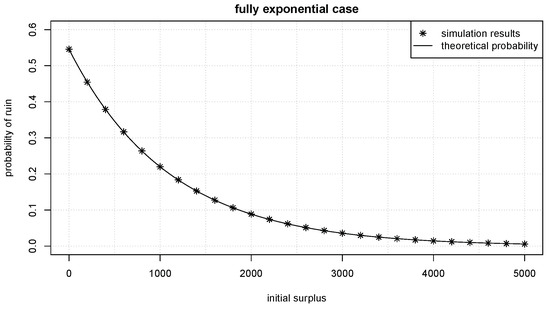
Suppose that the premiums are exponentially distributed with mean , and the claims are exponentially distributed with mean . This special case has been studied in Boikov (2003), where the author derived the exact ruin probability as
Consider the simulation approach. We simulate the transformed distribution of by simulating those of and separately. It is known that the Esscher transform of an exponential distribution is an exponential distribution. Hence, we have . On the other hand, consider the m.g.f. of the compound geometric random variable ,
where is the p.g.f. of , is the m.g.f. of , and is the probability of success of . The m.g.f. after the Esscher transform with parameter is then
Observing that Equation (25) has the same form as Equation (24), we conclude that the Esscher transformed compound geometric-exponential distribution is still a compound geometric-exponential distribution, with the compounding random variable being , and the compounded random variable being .
Now, all the components of the transformed surplus process may be simulated. Suppose , , , . It may be calculated that the adjustment coefficient . The theoretical probability of ruin by Equation (23) is then
We conduct the simulation study using 100,000 sample paths. The simulation results are plotted against the theoretical result in Figure 3, and one may see that they are perfectly aligned.
Figure 3.
Simulated probability of ruin vs. theoretical probability of ruin when both premiums and claims follow exponential distributions.
In the next example, we consider the case where the premium is a fixed amount, a. In some jurisdictions, the premiums for obligatory liability insurance are fixed or tiered, which may be modelled by the next example. We have the following lemma about this model.
Lemma 4.
If the premium is a constant, a, for each policy, and the claim size distribution is exponential with mean , then the probability of ultimate ruin is
where the adjustment coefficient, , is the root of the equation
Proof.
We first derive an integral equation satisfied by the survival probability . Considering the number of events in a small time interval , similarly to Boikov (2003), we have
Rearranging the terms of the latter equation yields
Dividing by and letting yields
One may verify that
is the solution to Equation (28), where the adjustment coefficient, , is determined by Equation (27). □
Example 2 (fixed premium amount per policy).
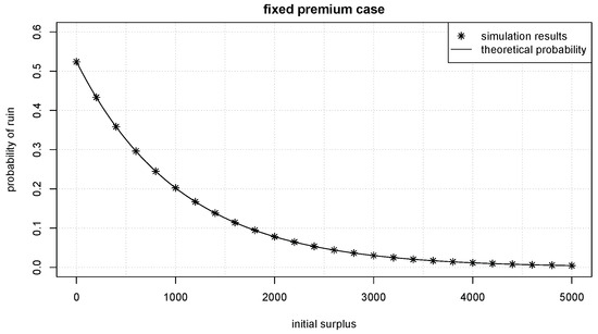
The simulation for this case is straightforward. The random variable is a linear combination of random variables. By Lemma 3, the transformed may be simulated by , where , and , where .
Suppose , it can be calculated that . A comparison of the simulated ruin probability and the theoretical ruin probability is given in Figure 4. Again, it is the case that they are aligned.
Figure 4.
Simulated ruin probability vs. theoretical ruin probability when premiums are fixed amounts.
The simulations in Examples 1 and 2 may be performed since the exact distribution of the Esscher transformed random variables may be identified. Specifically, the transformation of the compound random variable is known to be another compound random variable. This allows us to simulate it by simulating the compounding random variable and the compounded random variables sequentially. Notice that, in this case, one does not need the p.d.f. of to conduct the simulation. With arbitrary , the Esscher-transformed distribution may not be identifiable. In this case, only the m.g.f. of the new distribution is known, which is given by Equation (7). Some techniques exist for simulating random variables from moment generating functions. For example, McLeish (2014) discusses the use of the saddlepoint approximation to simulate a random variable from its m.g.f. Various possible different approaches are also compared therein. However, this type of approximation often relies on the assumption that the distribution is close to a known distribution, such as a normal distribution, and its accuracy varies in different settings. Taking advantage of the fact that the is a compound geometric distribution, we next present an approximation method based on the fast Fourier transform, which allows us to conduct the simulation for any appropriate premium-size distribution.
For the cases where the exact distribution of the Esscher transform of cannot be identified, the algorithm is:
- (i)
- Choose a sufficiently large truncation point, . Choose equally spaced , calculate
- (ii)
- Obtain a discretisation of using the fast Fourier transform.
- (a)
- Obtain , the fast Fourier transform of s.
- (b)
- Calculate as the approximation of the characteristic function.
- (c)
- Invert the fast Fourier transform to obtain . s are the discretisation of the compound distribution.
- (iii)
- Calculate the positive root, , to Equation (16).
- (iv)
- Simulate until , where is approximated by a discrete random variable, G, with . Return .
- (v)
- Repeat step (iv) sufficiently many times. The probability of ruin is the average of the return values.
The approximation approach has two main sources of error. The first source of error is discretisation. One may prove that the discretised random variable converges to the original random variable in distribution as the grid of the discretisation becomes finer, i.e., as approaches 0. The second source of error is the fast Fourier transform. To apply the fast Fourier transform, one needs to truncate the original distribution at the chosen truncation point, . Due to the periodic nature of the Fourier transform, the p.d.f. beyond point is “wrapped around” and appears in . This error is usually termed the aliasing error. For this reason, one should choose a sufficiently large , such that the p.d.f. beyond the truncation point is minimal to reduce the error. For demonstration, consider a compound Poisson-logarithmic distribution. It is known that this compound distribution is a negative binomial distribution. We obtain the mass function of the compound distribution using the fast Fourier transform with a different truncation point, . Since Poisson distribution is in the class, we may also obtain the mass function using Panjer’s recursion. The results are plotted in Figure 5. We observe that the aliasing error decreases as the truncation point, , increases. Both the fast Fourier transform and Panjer’s recursion can yield highly accurate approximations. However, it is known that the computation complexity of the fast Fourier transforms is , while the computation complexity of Panjer’s recursion is . When there are many points to evaluate, the fast Fourier transform has a computational advantage over Panjer’s recursion. For a more detailed comparison between the fast Fourier transform and Panjer’s recursion and an algorithm for reducing the aliasing error, see Embrechts and Frei (2009).
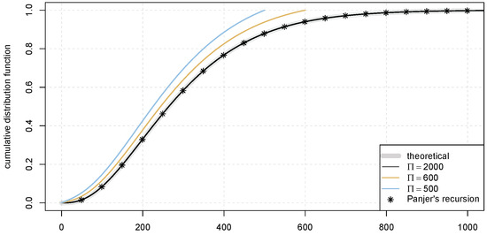
Figure 5.
Fast Fourier transform with aliasing error.
Example 3.
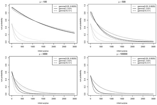
In this example, we consider gamma claim sizes and exponential premium sizes. For the claim process, let the intensity of be and let , so that ; for the premium process, let the intensity of be μ and let , so that , which implies a relative security loading of 1. We vary two key parameters of the model:
- α: this parameter controls the shape of the claim size distribution. Notice that, since the expected value of the claim size distribution is kept constant, the distribution has a heavier tail with a smaller α.
- μ: we let to observe the limiting behaviour of the model.
For each claim size distribution, we also consider the ruin probability under the classical model with the premium rate . Notice that this probability is not a function of μ. The truncation point, Π, used in the simulation is 1,000,000, at which point the survival function of the distribution of the compound random variable is sufficiently small. The simulation results with 100,000 simulated sample paths with and are given in Figure 6.
Figure 6.
Simulated ruin probability with gamma distributed claim sizes.
Remark 3.
Various known behaviours of the stochastic premium model may be observed in Example 3. For each gamma distribution, we see that the ruin probability under the stochastic premium model is greater than the ruin probability under the classical model for all u, regardless of μ. This is result 3 in Theorem 1. We also observe that, as μ increases, the ruin probability under the stochastic premium model converges to the ruin probability under the classical model, consistent with result 4 in Theorem 1.
Remark 4.
Some cases in Example 3 are extreme and unlikely to happen in practice. Notice that the expected number of premium arrivals in one period of time is . For an established insurer whose business does not vary dramatically on a year-to-year basis, μ is also approximately the portfolio size. Since all the claims are from the portfolio, the average number of claims per period of time from each policy is , which means that the average number of claims per policy is 10 when and is when . Based on some industry studies, such as APCIA et al. (2020), the claim frequency per exposure varies based on the physical environment and covered peril. As a result, we expect the impact of adopting the stochastic premium model to differ among different insurance portfolios.
5. An Example Using a Real-Life Data Set
We demonstrate the stochastic premium model with a real-life auto-insurance data set. The data set is provided by an industry partner who wishes to remain anonymous. The data set contains enough information for fully specifying a risk model. For a more detailed description of the data set, see Miao et al. (2023b).
We model the size and the frequency of premiums and claims separately. For the premium amount, it is determined that a 3-point mixture of normal distributions approximates the distribution well. The data set contains information on an insurance policy that is a combination of compulsory liability coverage and optional coverage. The premium for the compulsory liability coverage is determined by the class of the insured vehicle and past claim experience. The premium for the additional coverage is calculated using information that is more specific to the driver and the vehicle, such as the value of the vehicle and the region where the vehicle is mainly driven. This justifies the usage of mixture distribution: the three normal distributions are likely a result of three classes of vehicles, while within each class the premium varies due to the bonus–malus system and optional coverage. Using the maximum likelihood estimate, we obtain the parameters as
where s are normal density functions with
| mean | std | |||
| 1 | 0.10 | 1410 | 227 | |
| 2 | 0.41 | 2764 | 560 | |
| 3 | 0.49 | 4367 | 1716 |
Notice that the distribution is truncated at 0, hence the normalising constant. The left panel of Figure 7 presents the histogram of the observed premium amounts with the fitted density function.
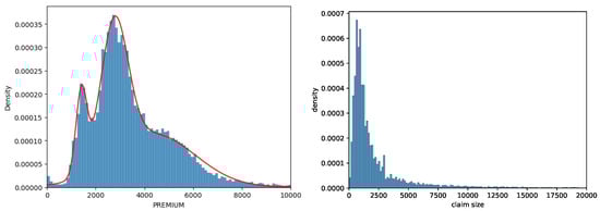
Figure 7.
(Left): histogram of the observed premium amounts with fitted density function. (Right): empirical distribution of the claim sizes.
The data set reveals distinct temporal patterns in the premium arrival process, including seasonality and growth trends. As noted in Miao et al. (2023b), these patterns alter the rate of premium arrivals, with fluctuations driven by recurring events such as policy renewals, periodic public events, and economic factors, along with long-term growth influenced by market expansion and demographic shifts. In this example, we simply use the average annual premium arrival as the intensity of , meaning that we assume premium arrivals occur at a steady rate throughout the year, disregarding the detailed seasonality and growth patterns. This simplification allows for easier analysis and computation. In this case, it is
which completes the modelling of the premium arrival process.
The claim amounts exhibit heavier tails than the premium amounts. This poses certain difficulties as the moment generating function of heavy-tailed distributions may not exist. For this example, we use the empirical distribution instead of trying to find a heavy-tailed parametric model. The right panel of Figure 7 illustrates the empirical distribution of the claim sizes.
A key quantity to determines the relationship between the premium arrival process and the claim arrival process is the claim rate per exposure. To this end, we calculate the number of claims as well as the in-force exposure on each day. The daily claim rate is calculated as the ratio of the two and is given in Figure 8. The daily claim rate is then converted to the annual rate. More specifically, each exposure generates 0.314201 claims per year. As a result, we have
and the claim process is also fully specified.
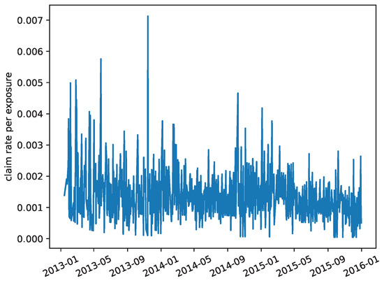
Figure 8.
Daily claim rate per exposure.
We also examine the classical risk model to show the differences the stochastic premium model makes. The comparable classical risk model (1) has the premium rate
Probabilities of ruin are simulated under both models with a different initial surplus. The results are given in Figure 9 as the blue and the orange curves.
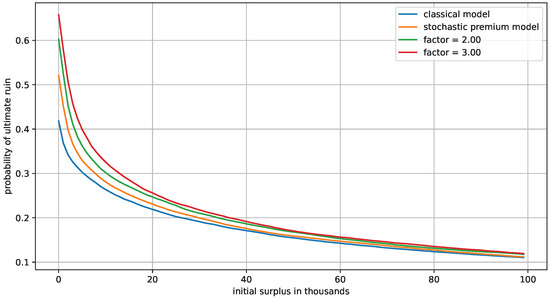
Figure 9.
Comparison of probability of ruin under the classical model and the stochastic premium model using the auto-insurance data set.
Consistent with Theorem 1, the probability of ruin is higher under the stochastic premium model than the classical model. The required reserves for the insurance company to control the probability of ruin with different risk levels are given in Table 1 in the column . We note that the stochastic premium model is a more conservative model that yields a higher reserve requirement, although in this specific case the average number of claims per exposure is not high, and therefore the classical model and the stochastic premium model are not extremely different.

Table 1.
Initial surplus required to limit the probability of ruin.
Application of the Model under Other Scenarios
An interesting comparison we can make is allowing the average claim rate per exposure to vary. In the example using the real-life auto-insurance data set, we multiply the average claim rate per exposure by a constant, . We also scale the premium size distribution accordingly such that the relative security loading remains constant. The modified risk process is then , where , and is a Poisson process with intensity . We choose and 3 to demonstrate the difference it makes. Under the classical model, the probability of ruin depends only on the relative security loading and the claim size distribution. Consequently, the results under the classical model remain constant regardless of the value of . The results under the stochastic premium model are simulated using the method in Section 4, and the level of initial surplus required to control the probability of ruin is given in Table 1. We observe that the difference between the classical model and the stochastic premium model increases as increases. Moreover, for each , the percentage difference is larger if the insurance company has higher risk tolerance.
As noted in Werner and Modlin (2010), it is a standard practice in ratemaking to adjust future premiums based on historical claim data. When insurers observe a higher-than-expected number of claims per exposure, they typically respond by raising premiums to cover the increased costs. However, from a risk management perspective, merely increasing premiums does not fully address the risk of insolvency. As illustrated by the results in Table 1, a higher average claim rate not only raises expected liabilities but also amplifies the relative uncertainty of the premium income. This means that higher reserves are necessary to maintain the same risk level. For practitioners, accounting for uncertainties in both the timing and amount of premiums and claims yields a better description of their insolvency risk. Compared with the classical model, the stochastic premium model more accurately reflects real-world conditions. This makes it a more realistic tool for evaluating insolvency risk and is one advantage of the stochastic premium model.
In practice, the changes in the physical environment often alter the actual claim experience. For example, Richardson and Hartman (2022) used dynamic linear models to study the impact of the COVID-19 pandemic on the auto-insurance industry. It was discovered that the frequency of claims was lower while the severity was higher during the pandemic, likely due to fewer miles driven. Since the claim rate is lower, it is likely that the difference between the classical model and the stochastic premium model is smaller. This is one example where an external factor affects the claim rate per exposure.
Another better studied example is the increasing frequency of claims for property and casualty insurance. Due to climate change, extreme weather events are becoming more frequent and more severe, leading to a heavy burden on communities across the globe. Its impacts on insurance practices have attracted more attention in recent years. Using Canada as an example, insurers are incurring more losses due to climate change in recent years. Figure 10 illustrates the total inflation-adjusted loss and the number of catastrophic events over the past four decades (source: Insurance Bureau of Canada (2023)). Both the total loss and the number of events has increased significantly in this time period.
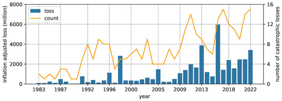
Figure 10.
Total annual inflation-adjusted catastrophic losses and number of catastrophic events in Canada.
One way an extreme weather event could impact insurance companies is by causing a large volume of claims to arrive at the same time. An early example of this is Hurricane Andrew, which struck the Bahamas and part of the US in 1992. The large losses caused at least 16 insurance companies to go bankrupt. This prompted regulatory changes that imposed stricter solvency requirements on insurers. Nowadays, it is a common practice for insurers to manage their exposure to catastrophe losses through more prudent risk selection and the use of reinsurance contracts. This focuses on the tail distribution of the aggregate claim.
The results presented in this paper reveal another possible impact that climate change may have on insurance companies, namely an increased claim rate in day-to-day non-catastrophic claims. As meteorological studies point out, climate change also alters the patterns of more localised events, such as flash floods, hail, and landslides; see, for example, Kleinen and Petschel-Held (2007); Raupach et al. (2021); and Gariano and Guzzetti (2016). These events are likely to increase the claim rate per policy, but not likely to result in insolvency in the short term. The results of this paper suggest that, in addition to adjustments to the premium rate, an insurer needs to have a higher level of reserves to achieve the same risk level. Naturally, climate change would alter the demand for insurance, as well as claim size distribution. This requires the insurers to re-evaluate their insolvency risk using the best estimates that take into consideration the new patterns in premiums and claims.
The stochastic premium model considers the uncertainty in both premiums and claims. As demonstrated in this paper, this may contribute to a better understanding of an insurer’s insolvency risk. By adopting the stochastic premium model, insurance companies can better withstand the pressures associated with uncertain future cashflow, which in turn may contribute to a better financial resilience and stability. Insolvency of insurers can destabilise the market and leave policyholders vulnerable, such as in the catastrophic scenario after Hurricane Andrew. The ability to proactively adjust reserves and premiums using more sophisticated risk models not only protects the insurer’s solvency but also provides policyholders with more secure and reliable coverage. This is a potential societal benefit of the proposed method in this paper.
6. Conclusions
In this paper, we investigate the application of the stochastic premium model. We first derive a simulation approach to obtain the probability of ruin. A new probability measure is defined through the Esscher transform under which ruin is certain. The simulation is carried out under the new probability measure, and the probability of ruin under the original probability measure is obtained. For cases where the sampling distribution is not identifiable, we take advantage of the fact that the drop of surplus may be expressed as a compound geometric distribution and use the fast Fourier transform as an approximation. Some theoretical results pertinent to this model are reviewed and demonstrated through examples.
By using special cases whose theoretical probability of ruin is known, we discover that the simulation approach is fast and is capable of producing highly accurate results. The simulation approach may be readily extended to more general cases as well. We also discover that the differences between the stochastic premium model and the classical model vary based on a number of factors, such as the heaviness of tail of the distributions and the claim frequency per exposure. This indicates that the impact of adopting the stochastic premium model varies among different insurance portfolios and that the applicability of this model in practice is worth further investigation.
We demonstrate the impact of using the model in practice through a real-life auto-insurance example. After fitting the model to the data, we use the probability of ruin as a risk measure to compare the performance of the stochastic premium model and the classical model. We also present the amount of initial surplus required to control the insolvency risk as a more intuitive and practical measure. We discover that, albeit the results are consistent with the known results in theory, the practical differences are marginal for this specific data set. This is due to the fact that the claim rate per exposure is relatively low. We explore other hypothetical scenarios using modified versions of the data set. More specifically, we investigate whether a worsening claim experience further differentiates the two models. We discover that, in a changing physical environment where the claim rate is higher, simply increasing the premium to counter the increased claims is not sufficient for insurers to control their insolvency risk adequately. As the claim rate increases, the risk associated with the uncertainty of premium income becomes more pronounced. As a result, insurers need to have more surplus to account for this increased risk. As external factors such as climate change, COVID-19, and urbanisation alter the demand for insurance and the claim experience for each policy, the insolvency risk may be re-evaluated using the latest estimates that account for changes in both premiums and claims. This highlights the potential practical value of the stochastic premium model in an ever-evolving environment.
Author Contributions
Conceptualization, Y.M. and K.P.S.; methodology, Y.M. and K.P.S.; software, Y.M.; validation, Y.M. and K.P.S.; formal analysis, Y.M.; investigation, Y.M.; resources, Y.M. and K.P.S.; data curation, Y.M.; writing—original draft preparation, Y.M.; writing—review and editing, Y.M. and K.P.S.; visualization, Y.M.; supervision, K.P.S.; funding acquisition, K.P.S. All authors have read and agreed to the published version of the manuscript.
Funding
This research was enabled in part by support provided by Compute Ontario (www.computeontario.ca) and the Digital Research Alliance of Canada (alliancecan.ca). Support from the Natural Sciences and Engineering Research Council of Canada for this work is gratefully acknowledged by Kristina Sendova.
Data Availability Statement
Acknowledgments
The authors would like to thank Junxiu Liu, FSA, FCIA, for fruitful discussions on current actuarial practices and regulations.
Conflicts of Interest
The authors declare no conflicts of interest.
References
- Albrecher, Hansjörg, and Søren Asmussen. 2006. Ruin probabilities and aggregrate claims distributions for shot noise cox processes. Scandinavian Actuarial Journal 2006: 86–110. [Google Scholar] [CrossRef]
- Albrecher, Hansjörg, Hans U. Gerber, and Hailiang Yang. 2010. A direct approach to the discounted penalty function. North American Actuarial Journal 14: 420–34. [Google Scholar] [CrossRef][Green Version]
- Albrecher, Hansjörg, Jan Beirlant, and Jozef L Teugels. 2017. Reinsurance: Actuarial and Statistical Aspects. Hoboken: John Wiley & Sons. [Google Scholar]
- Albrecher, Hansjörg, José Carlos Araujo-Acuna, and Jan Beirlant. 2021. Fitting nonstationary cox processes: An application to fire insurance data. North American Actuarial Journal 25: 135–62. [Google Scholar] [CrossRef]
- Andersen, E. Sparre. 1957. On the collective theory of risk in case of contagion between claims. Bulletin of the Institute of Mathematics and its Applications 12: 275–79. [Google Scholar]
- APCIA, CAS, and SOA. 2020. Auto Loss Cost Trends 2019 Update. Available online: https://www.soa.org/resources/research-reports/2020/auto-loss-cost/ (accessed on 29 September 2024).
- Asmussen, Soren, and Hansjorg Albrecher. 2010. Ruin Probabilities. Singapore: World Scientific, vol. 14. [Google Scholar]
- Asmussen, Søren. 1989. Risk theory in a markovian environment. Scandinavian Actuarial Journal 1989: 69–100. [Google Scholar] [CrossRef]
- Asmussen, Søren, and Klemens Binswanger. 1997. Simulation of ruin probabilities for subexponential claims. ASTIN Bulletin: The Journal of the IAA 27: 297–318. [Google Scholar] [CrossRef]
- Asmussen, Søren, and Peter W Glynn. 2007. Stochastic Simulation: Algorithms and Analysis. New York: Springer Science & Business Media, vol. 57. [Google Scholar]
- Asmussen, Søren, and Tomasz Rolski. 1994. Risk theory in a periodic environment: The cramer-lundberg approximation and lundberg’s inequality. Mathematics of Operations Research 19: 410–33. [Google Scholar] [CrossRef]
- Avanzi, Benjamin, Greg Taylor, Bernard Wong, and Alan Xian. 2021a. Modelling and understanding count processes through a markov-modulated non-homogeneous poisson process framework. European Journal of Operational Research 290: 177–95. [Google Scholar] [CrossRef]
- Avanzi, Benjamin, Greg Taylor, Bernard Wong, and Xinda Yang. 2021b. On the modelling of multivariate counts with cox processes and dependent shot noise intensities. Insurance: Mathematics and Economics 99: 9–24. [Google Scholar] [CrossRef]
- Boikov, Andrey V. 2003. The cramér–lundberg model with stochastic premium process. Theory of Probability & Its Applications 47: 489–93. [Google Scholar]
- Brigham, E. Oran. 1988. The Fast Fourier Transform and Its Applications. Englewood Cliffs: Prentice-Hall, Inc. [Google Scholar]
- Bucklew, James. 2013. Introduction to Rare Event Simulation. New York: Springer Science & Business Media. [Google Scholar]
- Bühlmann, Hans, Freddy Delbaen, Paul Embrechts, and Albert N. Shiryaev. 1998. On Esscher transforms in discrete finance models. ASTIN Bulletin 28: 171–86. [Google Scholar] [CrossRef]
- Chuang, Shuo-Li, and Patrick L Brockett. 2014. Modeling and pricing longevity derivatives using stochastic mortality rates and the Esscher transform. North American Actuarial Journal 18: 22–37. [Google Scholar] [CrossRef]
- Cooley, James W., and John W. Tukey. 1965. An algorithm for the machine calculation of complex fourier series. Mathematics of Computation 19: 297–301. [Google Scholar] [CrossRef]
- Dassios, Angelos, and Ji-Wook Jang. 2003. Pricing of catastrophe reinsurance and derivatives using the cox process with shot noise intensity. Finance and Stochastics 7: 73–95. [Google Scholar] [CrossRef]
- Dassios, Angelos, Jiwook Jang, and Hongbiao Zhao. 2015. A risk model with renewal shot-noise cox process. Insurance: Mathematics and Economics 65: 55–65. [Google Scholar] [CrossRef]
- Elliott, Robert J, Leunglung Chan, and Tak Kuen Siu. 2005. Option pricing and esscher transform under regime switching. Annals of Finance 1: 423–32. [Google Scholar] [CrossRef]
- Embrechts, Paul, and Marco Frei. 2009. Panjer recursion versus fft for compound distributions. Mathematical Methods of Operations Research 69: 497–508. [Google Scholar] [CrossRef]
- Gariano, Stefano Luigi, and Fausto Guzzetti. 2016. Landslides in a changing climate. Earth-Science Reviews 162: 227–252. [Google Scholar] [CrossRef]
- Gerber, Hans U., and Elias SW Shiu. 1998. On the time value of ruin. North American Actuarial Journal 2: 48–72. [Google Scholar] [CrossRef]
- Grandell, Jan. 2012. Aspects of Risk Theory. New York: Springer Science & Business Media. [Google Scholar]
- Grübel, Rudolf, and Renate Hermesmeier. 1999. Computation of compound distributions i: Aliasing errors and exponential tilting. ASTIN Bulletin: The Journal of the IAA 29: 197–214. [Google Scholar] [CrossRef]
- Hardy, Mary R. 2006. Approximating the aggregate claims distribution. Encyclopedia of Actuarial Science 1: 76–86. [Google Scholar]
- Insurance Bureau of Canada. 2023. 2023 Facts of the P&C insurance Industry in Canada. Available online: https://www.ibc.ca/industry-resources/resources-data/facts-book/ (accessed on 29 September 2024).
- Kleinen, Thomas, and Gerhard Petschel-Held. 2007. Integrated assessment of changes in flooding probabilities due to climate change. Climatic Change 81: 283–312. [Google Scholar] [CrossRef]
- Klugman, Stuart A, Harry H Panjer, and Gordon E Willmot. 2012. Loss Models: From Data to Decisions. Hoboken: John Wiley & Sons, vol. 715. [Google Scholar]
- Labbé, Chantal, and Kristina P Sendova. 2009. The expected discounted penalty function under a risk model with stochastic income. Applied Mathematics and Computation 215: 1852–67. [Google Scholar] [CrossRef]
- Lu, Yi, and Shuanming Li. 2005. On the probability of ruin in a markov-modulated risk model. Insurance: Mathematics and Economics 37: 522–32. [Google Scholar] [CrossRef]
- McLeish, Don. 2014. Simulating random variables using moment-generating functions and the saddlepoint approximation. Journal of Statistical Computation and Simulation 84: 324–34. [Google Scholar] [CrossRef]
- Miao, Yang, Kristina P. Sendova, and Bruce L. Jones. 2023a. On a risk model with dual seasonalities. North American Actuarial Journal 27: 166–84. [Google Scholar] [CrossRef]
- Miao, Yang, Kristina P. Sendova, Bruce L. Jones, and Zhong Li. 2023b. Some observations on the temporal patterns in the surplus process of an insurer. British Actuarial Journal 28: e4. [Google Scholar] [CrossRef]
- Morales, Manuel. 2004. On a surplus process under a periodic environment: A simulation approach. North American Actuarial Journal 8: 76–89. [Google Scholar] [CrossRef]
- Osgood, Brad G. 2019. Lectures on the Fourier Transform and Its Applications. Providence: American Mathematical Society, vol. 33. [Google Scholar]
- Pham, Huyên. 2007. Some applications and methods of large deviations in finance and insurance. In Paris-Princeton Lectures on Mathematical Finance 2004. Berlin: Springer, pp. 191–244. [Google Scholar]
- Raupach, Timothy H., Olivia Martius, John T. Allen, Michael Kunz, Sonia Lasher-Trapp, Susanna Mohr, Kristen L. Rasmussen, Robert J. Trapp, and Qinghong Zhang. 2021. The effects of climate change on hailstorms. Nature Reviews Earth & Environment 2: 213–26. [Google Scholar]
- Richardson, Robert, and Brian Hartman. 2022. Examining Auto Loss Trends through the Covid Pandemic. Available online: https://www.soa.org/resources/research-reports/2022/auto-loss-trends-covid/ (accessed on 29 September 2024).
- Sundt, Bjørn, and William S Jewell. 1981. Further results on recursive evaluation of compound distributions. ASTIN Bulletin: The Journal of the IAA 12: 27–39. [Google Scholar] [CrossRef]
- Temnov, Gregory. 2004. Risk process with random income. Journal of Mathematical Sciences 123: 3780–94. [Google Scholar] [CrossRef]
- Vidmar, Matija. 2018. Ruin under stochastic dependence between premium and claim arrivals. Scandinavian Actuarial Journal 2018: 505–13. [Google Scholar] [CrossRef]
- Werner, Geoff, and Claudine Modlin. 2010. Basic Ratemaking. Available online: https://www.casact.org/abstract/basic-ratemaking (accessed on 29 September 2024).


Disclaimer/Publisher’s Note: The statements, opinions and data contained in all publications are solely those of the individual author(s) and contributor(s) and not of MDPI and/or the editor(s). MDPI and/or the editor(s) disclaim responsibility for any injury to people or property resulting from any ideas, methods, instructions or products referred to in the content. |
© 2024 by the authors. Licensee MDPI, Basel, Switzerland. This article is an open access article distributed under the terms and conditions of the Creative Commons Attribution (CC BY) license (https://creativecommons.org/licenses/by/4.0/).