Article

The Italian Actuarial Climate Index: A National Implementation Within the Emerging European Framework

by
Barbara Rogo
1,*,
José Garrido
2 and
Stefano Demartis
1
1
Department of Statistical Sciences, Sapienza University of Rome, 00185 Rome, Italy
2
Department of Mathematics and Statistics, Concordia University, Montreal, QC H3G 1M8, Canada
*
Author to whom correspondence should be addressed.
Risks 2025, 13(10), 192; https://doi.org/10.3390/risks13100192
Submission received: 7 August 2025 / Revised: 18 September 2025 / Accepted: 28 September 2025 / Published: 3 October 2025
(This article belongs to the Special Issue Climate Change and Financial Risks)

Abstract

This paper presents the development of a high-resolution composite index to monitor and quantify climate-related risks across Italy. The country’s complex climatic variability, extensive coastline, and low insurance penetration highlight the urgent need for robust, locally calibrated tools to bridge the climate protection gap. Building on the methodological framework of existing actuarial climate indices, previously adapted for France and the Iberian Peninsula, the index integrates six standardised indicators capturing warm and cool temperature extremes, heavy precipitation intensity, dry spell duration, high wind frequency, and sea level change. It leverages hourly ERA5-Land reanalysis data and monthly sea level observations from tide gauges. Results show a clear upward trend in climate anomalies, with regional and seasonal differentiation. Among all components, sea level is most strongly correlated with the composite index, underscoring Italy’s vulnerability to marine-related risks. Comparative analysis with European indices confirms both the robustness and specificity of the Italian exposure profile, reinforcing the need for tailored risk metrics. The index can support innovative risk transfer mechanisms, including climate-related insurance, regulatory stress testing, and resilience planning. Combining scientific rigour with operational relevance, it offers a consistent, transparent, and policy-relevant tool for managing climate risk in Italy and contributing to harmonised European frameworks.

1. Introduction

Climate-related risks have become a defining challenge of the contemporary era, generating increasingly severe and widespread impacts across social and economic systems. These impacts often interact and reinforce one another, creating feedback loops of environmental degradation, economic loss, and social vulnerability. Rising temperatures, shifting seasonal patterns, droughts, floods, wildfires, and sea level rise are disrupting agricultural production, threatening ecosystems, straining healthcare systems, and exposing critical infrastructure. The challenge is particularly acute for countries such as Italy, where exposure and vulnerability often coincide. Vulnerable groups, with limited capacity to adapt or respond, are disproportionately affected, resulting in heightened inequalities and, in some cases, migration pressures. The loss of biodiversity and the degradation of natural ecosystems further weaken territorial resilience, amplifying the risk of systemic disruption in the face of environmental shocks.
Climate-related risks are increasingly challenging the sustainability of insurance business models and solvency positions. The growing frequency and intensity of natural disasters is putting pressure on underwriting performance, increasing claims costs, and exposing the limitations of traditional actuarial models. At the same time, uncertainty about future climate trajectories complicates capital allocation and long-term pricing decisions, with significant implications for solvency and profitability. These issues are especially critical for insurers, who operate both as risk carriers and long-term institutional investors. According to (Mills 2005), the combined effect of escalating catastrophe losses, higher capital costs, and inflation in reconstruction expenses has resulted in a growing number of years in which insurers have recorded negative technical results. This fragility is often exacerbated by the persistent underestimation of climate-related risks, which leads to chronic underpricing and reliance on financial returns to offset underwriting losses, a practice referred to as cash-flow underwriting, that is, reliance on investment income to offset technical losses. When major catastrophic events coincide with downturns in financial markets, such exposure can trigger severe liquidity stress and systemic spillovers, as studied by (Zhou et al. 2023). Recent empirical evidence confirms that climate risk can undermine financial stability. Based on data from 53 countries, (Liu et al. 2024) show that the impact varies across economic and financial systems, reinforcing the need to integrate climate considerations into macroprudential supervision.
Recent regulatory developments place increasing emphasis on the integration of sustainability risks, including physical risks arising from climate change, into insurers’ governance and risk management frameworks. European regulations have introduced explicit requirements for incorporating these risks into the governance system and the assessment of overall solvency needs (European Commission 2015, 2021). These provisions have been transposed into the Italian regulatory framework through revisions to national supervisory rules, which provided a formal definition of sustainability risks and required their integration into the risk management system and strategic objectives of insurance undertakings (IVASS 2021). In addition, the actuarial function has been assigned a new responsibility, specifically to provide an opinion on sustainability-related risks as part of the underwriting policy assessment.
In line with these requirements, the European Insurance and Occupational Pensions Authority (EIOPA) further emphasises the importance of integrating climate-related physical risks into the Own Risk and Solvency Assessment (ORSA) and capital adequacy assessments. In its supervisory guidance (EIOPA 2019, 2022), EIOPA calls for forward-looking, scenario-based approaches and highlights the need to consider the long-term impact of climate change on insurers’ solvency positions and risk profiles.
The Italian territory is particularly exposed to climate-related risks due to its geographic configuration, high population density, and the concentration of economic activity in vulnerable areas such as coastal zones, floodplains, and urban areas. A significant share of the country’s infrastructure, agricultural land, and cultural heritage is located in areas exposed to sea level rise, river flooding, landslides, and heatwaves. These physical vulnerabilities are compounded by structural weaknesses in Italy’s climate risk protection system, as evidenced by the persistent gap between total economic and insured losses following major catastrophic events. One of the most striking examples is the flood that struck the Emilia Romagna region in May 2023, a densely populated and industrialised area in northern Italy, which resulted in an estimated 9.8 billion USD in economic losses, with only 600 million USD covered by insurance. According to Aon (2024), it ranked as the sixth costliest natural disaster worldwide that year. This episode underscores a persistent and substantial protection gap in a context of rising climate extremes.
In addition to direct physical and economic impacts, climate change is expected to generate wider systemic repercussions for Italy’s macroeconomic and financial stability. The Bank of Italy has been actively involved in assessing climate-related risks using NGFS scenarios (Aiello et al. 2024), highlighting potential long-term effects, including lower GDP growth, rising inflationary pressures, and heightened financial market volatility. These insights underscore the urgency of providing financial actors with forward-looking tools to capture the physical dimension of climate risk. In Italy, where geographic exposure coincides with structural protection gaps, the availability of high-resolution, context-sensitive indicators is particularly crucial for effective risk governance and the design of informed public policies.
The growing complexity and territorial variability of climate-related risks highlight the need for analytical tools to support forward-looking assessments of exposure, insurance pricing, and policy design. One of the most promising approaches is the development of actuarial climate indices, such as the Actuarial Climate Index (ACI), developed by North American actuarial associations. The ACI provides a synthetic and standardised representation of climate-related anomalies relative to historical baselines. It quantifies the intensification of extreme events, including warm and cold temperature extremes, droughts, heavy precipitation, wind, and sea level rise, through seasonally disaggregated components that are then combined into a single composite index.
Such indices assist regulators and public authorities in monitoring the evolution of physical risks over time and across regions. In the insurance domain, they may also help inform pricing strategies, capital planning, and the design of parametric solutions, particularly within multi-hazard schemes or public–private risk-sharing arrangements. In Italy, the absence of operational, high-resolution indicators tailored to the physical dimension of climate risk remains a significant barrier to the effective integration of these risks into actuarial models, financial supervision, and public governance.
Against this backdrop, the development of a dedicated national index tailored to Italy’s specific territorial and climatic conditions can make a meaningful contribution to bridging the existing information gap and enhancing climate risk awareness and preparedness. A reliable, high-resolution indicator system is particularly valuable for supporting risk-sensitive decision-making by insurers, regulators, and public authorities.
In this perspective, the insurance sector plays a pivotal role in climate risk governance. Beyond providing financial protection through risk transfer mechanisms, insurers can foster risk-aware behaviours (by aligning insurance costs with individual risk exposure), encourage investment in resilience (through premium discounts for adaptive measures), and promote a culture of prevention (by contributing to public–private risk-planning frameworks). Empirical evidence supports these functions. A recent study by Cheung et al. (2024) analyses the long-term relationship between extreme weather variables in the ACI and agricultural yields, identifying a significant link between sea level rise and crop productivity. The authors propose a hybrid bonus–malus mechanism that distinguishes between damages caused by extreme weather events and those attributable to policyholder behaviour, with the aim of avoiding unfair penalties for losses beyond the insured’s control, while also promoting more risk-aware conduct and enhancing both the fairness and effectiveness of insurance-based climate risk management.
However, the persistent protection gap observed in Italy highlights the need for renewed coordination between public policy and private insurance instruments. Public–private partnerships and national risk-sharing mechanisms can enhance financial preparedness and ensure a more equitable distribution of climate-related losses. These arrangements are particularly relevant in high-risk areas where market-based solutions alone may be insufficient, and where the involvement of public actors can strengthen both coverage and affordability.
Among the instruments available to expand insurance coverage and accelerate post-disaster liquidity, parametric insurance products are attracting growing attention. These policies provide predefined payouts based on the occurrence of specific events or the exceedance of measurable thresholds (such as temperature, rainfall, or wind speed), without requiring individual loss assessments. By reducing transaction costs and response times, parametric schemes are well-suited to climate-related risks, especially when supported by robust indicators such as actuarial climate indices. Cheung et al. (2024) demonstrate that the variables included in the ACI can serve as trigger parameters within index-based insurance schemes. A comprehensive review of parametric insurance is provided by Lin and Kwon (2020), who examine contract types, current market practices, and the main advantages and limitations compared with indemnity-based models. Figueiredo et al. (2018) propose a probabilistic framework for parametric trigger modelling based on logistic regression, addressing basis risk, defined as the mismatch between actual losses and predefined payouts.
More recently, a number of contributions have highlighted the growing importance of climate risk assessment and index-based solutions in both actuarial and applied fields. Hernández-Rojas et al. (2023) demonstrate that data-driven methodologies, particularly deep neural networks built on high-frequency satellite climate indices, can outperform traditional statistical models in constructing weather index insurance and reducing basis risk. De Vivo et al. (2023) apply a comprehensive climate risk assessment framework to major Italian airports, integrating reanalysis indicators, climate projections, and vulnerability data to evaluate risks from extreme precipitation events. Lomelì-Quintero et al. (2023) develop a georeferenced tool to quantify the economic impacts of sea level rise and coastal erosion in Catalonia, emphasising the crucial role of geomorphology and infrastructure in local risk assessments. Wijesena and Pradhan (2025) provide a systematic review of quantitative studies on Weather Index Insurance, highlighting the potential of machine learning, multi-index designs, and remote sensing data for improving risk transfer mechanisms. Finally, Gao and Shi (2025) propose a copula-based regression framework to capture spatial dependence in insurance claims from localised weather events, showing how such dependence critically shapes aggregate losses and claims management. These contributions confirm the timeliness of developing a nationally tailored actuarial climate index for Italy, capable of integrating climatic heterogeneity with insurance-related vulnerabilities.
Despite the growing literature on climate risk and the availability of ACI-based indices for France and the Iberian Peninsula, Italy still lacks a formally established index consistent with the ACI framework and capable of jointly capturing multi-hazard climate anomalies (including sea level) at high spatial resolution. This absence represents a critical gap for a country characterised by marked climatic heterogeneity and a persistent insurance protection gap. This paper addresses this gap by developing the Italian Actuarial Climate Index (ITACI) and (i) formalising a transparent aggregation framework aligned with the ACI family while introducing a specific treatment of the sea level component to reflect Italy’s distinctive exposure; (ii) providing national and sub-national analyses of temporal and spatial dynamics and (iii) offering a comparative perspective with the French Actuarial Climate Index (FACI) and the Iberian Actuarial Climate Index (IACI), highlighting Italy’s distinct marine signal in the Mediterranean context.
The ITACI is developed consistently with the ACI-based indices designed for Spain, Portugal (Zhou et al. 2023), and France (Garrido et al. 2024), contributing to a European-wide framework for monitoring physical climate risk and informing insurance and regulatory responses. These indices provide structured and transparent tools for assessing climate stress across time and space. In line with the regulatory definition of physical risk, which encompasses both acute events (such as floods, storms, or heatwaves) and chronic climatic shifts (including droughts and sea level rise)1, the ITACI combines multiple indicators that capture the frequency and severity of these phenomena. In a context marked by high exposure and persistent protection gaps, the ITACI contributes to enhancing national preparedness and resilience through data-driven climate risk governance. Moreover, the spatially flexible design of the ITACI enables its application at sub-national levels, including regional and local areas. This territorial granularity makes the index particularly valuable for supporting adaptation strategies, informing the pricing of insurance portfolios in vulnerable areas, and strengthening regional climate risk governance.
The paper is organised as follows: Section 2 motivates the development of a dedicated national index, while Section 3 outlines the methodological framework and the data sources employed in its construction. In Section 4, the component aggregation methodology is presented, focusing on computation across territorial units and the integration of the sea level component. Section 5 explores its temporal and spatial evolution, along with the dynamics of the underlying components at national and sub-area levels. Section 6 compares the index with its French and Iberian counterparts, with particular attention to the distinctive role of sea level dynamics in Italy, contrasting them with patterns observed in neighbouring countries. Finally, Section 7 summarises the main findings and discusses their implications for climate risk monitoring and insurance innovation. Appendices Appendix A and Appendix B provide additional spatial and regional insights that complement the main analysis.

2. Climate Risk Exposure and the Protection Gap in Italy

This section outlines the distinctive climatic and insurance-related characteristics of Italy that justify the construction of a national actuarial climate index. The country’s complex orography and extensive coastline generate marked spatial variability in climatic conditions, highlighting the importance of high-resolution monitoring. At the same time, the Italian insurance market shows persistent structural weaknesses in the coverage of natural catastrophes, particularly those associated with climate events. Taken together, these elements support the development of an index specifically calibrated to the country’s exposure profile and protection gaps.
Italy’s geographic configuration gives rise to pronounced climatic heterogeneity. The peninsula extends from approximately 47.1° N to 35.2° N in latitude and from 5.5° E to 18.7° E in longitude, encompassing the Alpine and Apennine mountain systems, Mediterranean coastal areas, and the two major islands of Sicily and Sardinia. The national territory covers about 301,000  km 2 , within which substantial spatial variability in climatic conditions can be observed.
Italy’s north–south orientation, peninsular shape, and complex topography accentuate spatial climatic contrasts and contribute to the occurrence of highly localised extreme events, particularly in coastal regions. These factors generate sharp climatic differences over relatively short distances. In addition, the country has a considerable coastal exposure of approximately 7900 km and is entirely surrounded by the semi-enclosed Mediterranean Sea, where sea level variability is driven mainly by regional atmospheric and oceanographic processes rather than by global-scale ocean currents.
A comparison with other European regions for which Actuarial Climate Indices have already been developed, namely France and the Iberian Peninsula, provides a useful context for the rationale behind a dedicated index for Italy. Both regions have a predominantly east–west orientation and are almost twice the size of Italy, with land areas of approximately 551,000 km 2 and 583,000 km 2 , respectively. Nonetheless, Italy’s coastline is significantly longer, extending to about 7900 km compared with 5500 km for France and 4900 km for the Iberian Peninsula. This difference is mainly attributable to Italy’s peninsular shape and highly indented shoreline. Furthermore, most of the coastline in France and the Iberian Peninsula faces the Atlantic Ocean (approximately 3400 km and 3900 km, respectively), a distinction that plays a critical role in the analysis of the sea level indicator.
Over the past decade, both the frequency and intensity of climate-related extreme events have increased significantly across Italy. The 2023 floods in Emilia-Romagna, together with recurrent flash floods in Liguria and Sicily, illustrate the growing instability of Italy’s climate regime. Figure 1 shows the number of extreme weather events recorded in Italy in 2013, 2017, and 2024, based on data from the LegAmbiente CittàClima map. In 2024, 356 events were recorded, nearly four times the figure reported in 2013 (95) and more than four and a half times that of 2017 (77).
The figure highlights the predominance of flood-related events, particularly those triggered by intense rainfall. A regional breakdown of the same dataset shows that Lombardy recorded the highest number in 2024, with 26 events. Droughts were also frequent, especially in Sicily (15) and Sardinia (9). As for urban heat extremes (2023 data), these were most often observed in Tuscany (6), followed by Sardinia and Sicily with 4 events each. These patterns confirm the regional variability of climate impacts and highlight the importance of high-resolution tools for supporting local-scale risk assessment and decision-making.
Despite increasing exposure to climate-related hazards, the Italian insurance market remains structurally underdeveloped in terms of natural catastrophe coverage, particularly for weather-related perils. Data from the EIOPA Protection Gap dataset2 confirm that Italy consistently shows low levels of insurance penetration across several categories of climate risk. For example, only 3% of the economic losses from flood events have historically been insured, while coastal flood losses show no insurance coverage at all.
Notably, Italy’s flood protection gap score is 2.5, reflecting both high exposure and structural underinsurance. According to EIOPA, this places the country among those requiring close monitoring. Together with Greece, Italy also records the highest aggregate protection gap score, with 12 out of 20 points. This score is based on five perils: flood, coastal flood, windstorm, wildfire, and earthquake, each contributing up to 4 points (see EIOPA 2024). Italy’s score has remained unchanged since 2022. By contrast, France and Spain reported significantly lower scores in 2024, at 6.5 and 6.0, respectively, despite facing comparable climate-related risks.
Recently, through Decree-Law No. 39/2025, the Italian government introduced a mandate requiring all businesses operating in the country to purchase a basic catastrophe insurance policy. This policy must cover material damage to assets used in business activities, specifically for earthquakes, floods, and landslides (IVASS 2025). The objective is to ensure a minimum level of universal protection, promote broad mutualisation, and contain premium costs, even in high-risk areas. The measure also aims to reduce the fiscal impact of climate-related economic losses by fostering risk sharing through the insurance market. While promising, the effects of this new mandate will need to be closely monitored as implementation unfolds.
It is important to note, however, that this obligation does not extend to private households, despite the substantial financial pressure they place on public finances. For instance, during the May 2023 floods in Emilia-Romagna, which caused 17 fatalities, damage to private homes accounted for nearly 24 percent of the total 8.86 billion euros in economic losses. Italian households remain largely uninsured against climate-related risks. According to ANIA (2024) estimates, as of March 2024, only 5.9 percent of residential units were insured against natural catastrophe risks, amounting to approximately 2.1 million out of 35.3 million dwellings. This underscores the urgent need to extend effective risk-transfer mechanisms to the residential sector.
A promising approach to expanding and improving insurance protection is the adoption of parametric (or index-based) insurance solutions. These instruments are increasingly recognised in both regulatory and academic contexts as a viable complement to traditional indemnity-based products3. Unlike conventional policies, parametric insurance links payouts to the exceedance of predefined thresholds in physical parameters, such as rainfall intensity, wind speed, or water level, or to composite indices derived from them. Once the trigger condition is met, a predetermined payout is automatically issued, irrespective of the actual economic loss incurred.
The effectiveness of a parametric product depends critically on the adequacy and reliability of the selected index. The trigger must be carefully calibrated to ensure that the payout corresponds closely to a high probability of actual loss. Otherwise, basis risk may arise when the compensation does not reflect the insured party’s actual damages. This underscores the importance of robust index design and local calibration, particularly in urban areas or regions highly exposed to climate-related hazards.
Parametric products offer several clear advantages, including predictable payouts, rapid liquidity, and the ability to cover risks that are otherwise difficult to insure through conventional mechanisms. When properly designed and calibrated, these instruments can effectively support public policy objectives by broadening the scope of insurable risks, enhancing the efficiency of financial response following disasters, and alleviating the fiscal burden on the State. These features are particularly relevant in a country like Italy, where the coexistence of diverse climatic exposures and low insurance penetration, combined with administrative constraints, may reduce the effectiveness of traditional compensation mechanisms. A concrete indication of growing institutional interest is the inclusion of parametric insurance among the eligible subsidised instruments for the agricultural sector in the 2024 Risk Management Plan (PGRA), marking a significant step towards integrating parametric approaches into national risk management strategies.
Empirical evidence supports the feasibility of index-based crop insurance in Southern Europe. Zhou and Vilar-Zanón (2024) demonstrate that the Spanish Actuarial Climate Index (SACI) is a reliable predictor of insurance losses for wine-grape growers affected by hailstorms, suggesting that climate indices can serve as effective triggers in parametric insurance schemes. A subsequent study by Zhou and Vilar-Zanón (2025) introduces a provincial version of the index (pSACI), revealing strong spatial heterogeneity in climate impacts and a significant correlation between pSACI and both the number of hailstorm claims and the associated losses. Similarly, Cheung et al. (2024) show that selected weather variables from the ACI exhibit long-term cointegration with crop yields and can be used as trigger parameters in pricing weather index insurance. These findings support further investigation into the potential use of ITACI in the design of climate risk-transfer instruments in Italy.
Building on this evidence, ITACI can provide a robust and operationally relevant basis for climate risk management in Italy. In addition to supporting the development and calibration of parametric products, it can serve as a national tool for systematic climate monitoring. By delivering high-quality, high-resolution, and regularly updated data, ITACI offers a transparent foundation for both public policies and private initiatives. Its capacity to synthesise multiple dimensions of climate anomalies makes it a credible benchmark for index-based insurance and broader climate-informed decision-making.
The analysis rests on a set of underlying premises. First, standardised climate anomalies are assumed to provide not only a consistent basis for temporal and spatial comparisons but also a means to render different variables comparable and to highlight statistically significant departures from the reference climate. Second, sea level is regarded as a critical dimension of climate risk in Italy, given the country’s extensive coastline. Third, combining multiple indicators into a single composite index is expected to enhance both the interpretability of climate dynamics and their relevance for insurance and regulatory applications.

3. Methodology Overview and Data Sources

The ITACI builds on the methodological framework originally developed for the ACI, launched in North America by the Canadian and U.S. actuarial associations. This approach has since been adopted in Europe through FACI and IACI, which cover both Spain and Portugal. The Italian implementation retains the core ACI structure, adapting it to the national context with geographically specific climate data. The following section outlines the sources, indicators, and processing procedures used.
The ITACI relies on the ERA5-Land reanalysis dataset, distributed via the Copernicus Climate Data Store (CDS), which provides hourly climate variables on a native 0.1 ° × 0.1 ° grid, corresponding to cells of approximately 88  km 2 over the Italian domain (Copernicus Climate Change Service (C3S) 2025). This high spatial resolution effectively captures the geographic and climatic heterogeneity of the Italian peninsula, as discussed in Section 2. The ITACI employs a set of indicators designed to capture climate extremes that are particularly relevant to actuarial risk analysis, including extremely high and low temperatures, heavy precipitation events, strong wind components, and prolonged droughts. In addition, it incorporates sea level anomalies derived from tide gauge observations provided by the Permanent Service for Mean Sea Level (PSMSL), specifically from the Revised Local Reference (RLR) dataset. This component is especially significant in the Italian context, where long coastal stretches and localised storm surges make sea level variability a key driver of risk.
These standardised indicators are then aggregated into composite monthly and seasonal indices, providing a quantitative measure of the severity and frequency of climate-related risks over time.
Each climate indicator is first computed at the level of individual grid cells, ensuring that local extremes are accurately captured before standardisation and temporal aggregation. By contrast, the sea level indicator is derived from monthly observations at fixed tide gauge stations located along the Italian coast and in adjacent areas of the central Mediterranean.
The construction of the ITACI indicators is based on a fully automated and modular workflow developed in Python (version 3.12.1). The entire process, from raw data extraction to the generation of indicator-level outputs, is designed to ensure robustness, efficiency, and full replicability, in line with best practices for quantitative and operational modelling. The workflow follows a structured sequence of operations, including data cleaning, transformation, and aggregation. All procedures have been implemented using a combination of standard open-source libraries (such as pandas, numpy, and xarray) and custom functions developed by the authors. These custom modules are specifically designed to handle high-resolution spatio-temporal climate data and to automate indicator computation within a reproducible framework. Parallel processing is employed during critical phases of the workflow to accelerate execution, particularly for data downloading and transformation. Quality assurance routines and error-handling mechanisms are embedded at each stage to ensure data integrity, traceability, and transparency. This computational framework supports the regular updating of the index and ensures its long-term operational sustainability.
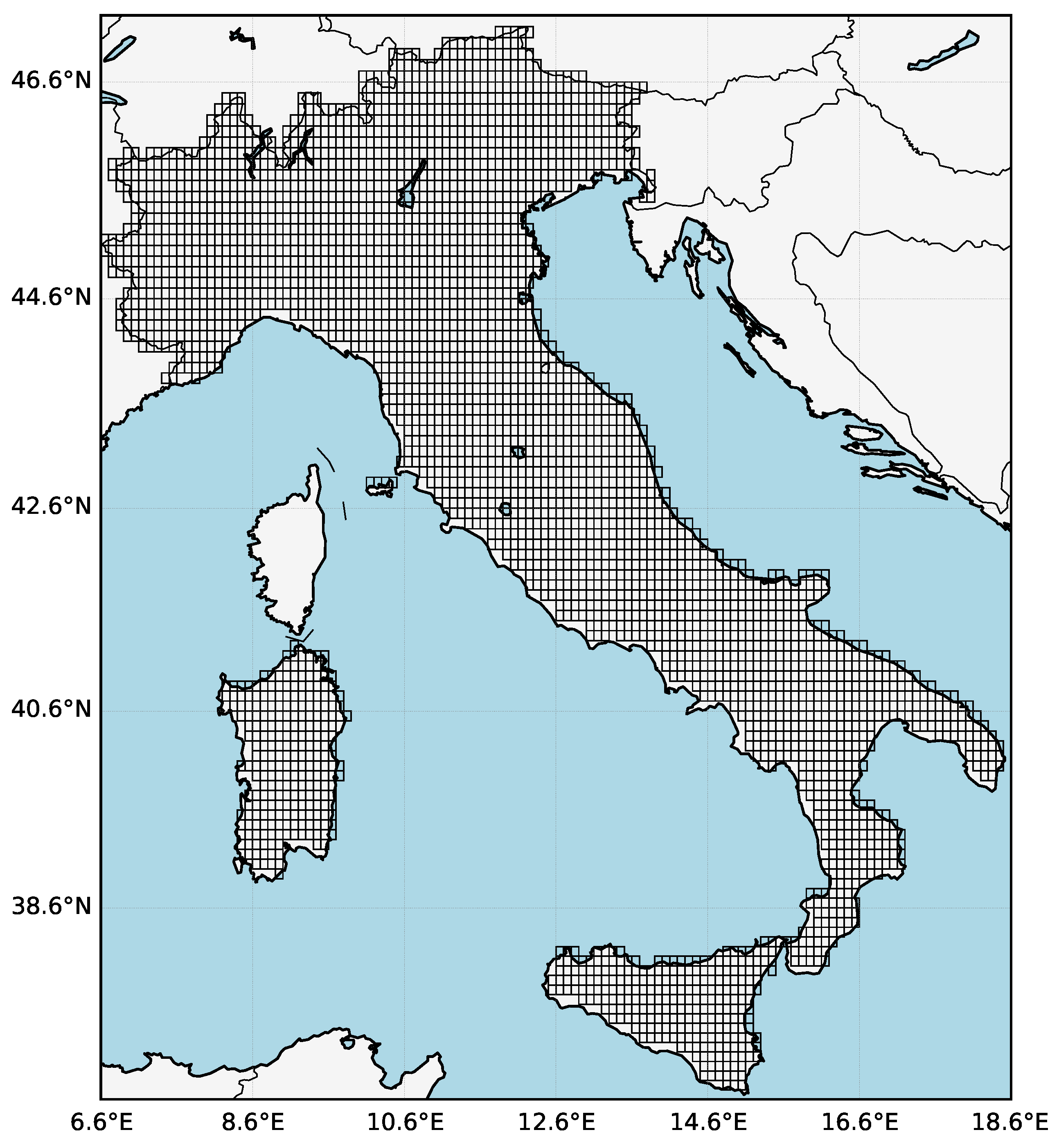
The dataset, containing the ERA5-Land-based variables, comprises hourly data from January 1961 to December 2024 and covers 3346 land grid cells across the Italian territory, as shown in Figure 2. The processed dataset consists of hourly observations for the following variables: 2-m air temperature (T), total precipitation (P), and the eastward ( W E ) and northward ( W N ) wind components at 10 metres. This amounts to over 1 billion individual records per climate variable, highlighting the need for a high-performance infrastructure capable of managing large-scale spatio-temporal data with precision and reliability.
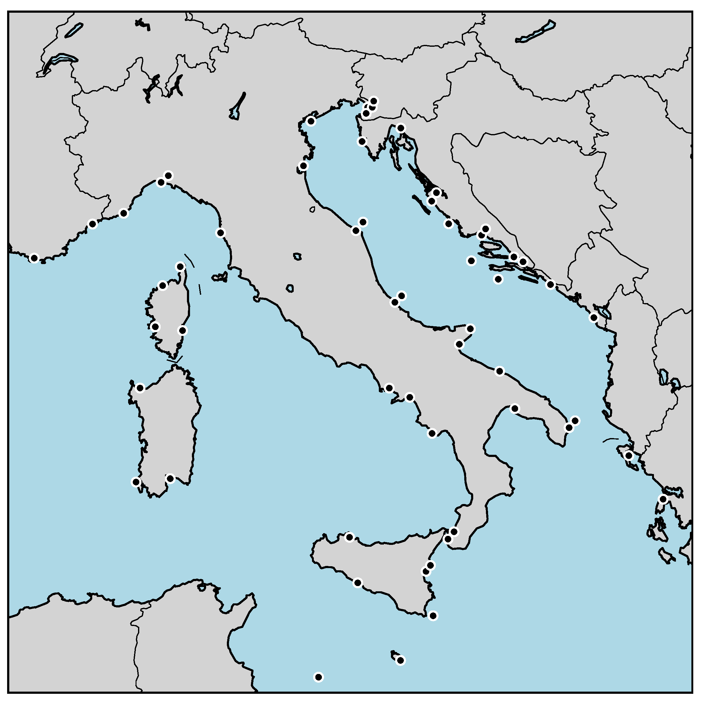
The sea level dataset comprises monthly values, expressed in millimetres relative to a fixed local reference, from 56 selected stations, as shown in Figure 3 (Permanent Service for Mean Sea Level 2025). The selection is based on georeferenced location and the availability of consistent time series without warning flags, such as those from the Monaco station. Evidence of systematic biases affecting long-term trends is also considered, as reported in Zerbini et al. (2017). In particular, the stations of Porto Corsini and Venice Punta Salute are excluded from the selection because the significant influence of local subsidence distorts the long-term sea level signal and renders these records unsuitable for inclusion in the ITACI reference baseline.
The sea level time series extend to 2023, representing the most up-to-date data available at the time of acquisition. To ensure index continuity for 2024, standardised sea level anomalies are held constant at their 2023 values until updated observations become available.
Table 1 provides a structured summary of the ITACI indicators used to characterise monthly and seasonal climate anomalies. For each indicator, the table specifies the underlying variable(s), the detection criterion adopted, and the aggregation rule applied to produce the corresponding monthly value. The detection criterion for temperature extremes is based on a centred moving window of ±2 calendar days around each day of the month, which captures local variability while smoothing daily fluctuations. Unlike atmospheric indicators, which are based on threshold exceedances or extreme values, the sea level component is defined using monthly mean anomalies. This reflects the fact that sea level variations are gradual and cumulative rather than short-lived extremes. Consequently, exceedance-based metrics, while suitable for variables characterised by sudden peaks such as precipitation or temperature extremes, add little value for sea level, whose variability is smooth and persistent over time.

4. Aggregation of Indicators for ITACI Computation

The ITACI computation involves the aggregation of climatic and sea level indicators, as detailed in Table 1. In line with the original methodology, each indicator contributes to the ITACI through its standardised anomaly, which indicates how far a value deviates from the reference mean in terms of a multiple of the reference standard deviation. This transformation allows variables with different units to be compared on a common scale. For climatic indicators, anomalies are computed at the grid-cell level, whereas the sea level anomaly is calculated for the entire area.
Let A I denote a sub-area of the total area I , which represents Italy, including its islands. Let G = i = 1 n A C i , where each C i denotes an individual grid cell. We refer to G as the cell grid associated with the sub-area A , and write A G to indicate that the set of cells G provides an approximate spatial representation of A . The ITACI value for the area A , in month j and year l, is defined as follows:
ITACI A ( j , l ) = 1 ω A X X a X A ( j , l ) + ω S A a S ( j , l ) ,
where ω A = 5 + ω S A , with ω S A denoting the weight assigned to the sea level indicator for sub-area A (further discussed below), and X = { F warm , F cool , P max , L dry , F wind } . The standardised anomaly a X A ( j , l ) of the indicator X X for the area A , is given by the following:
a X A ( j , l ) = X A ( j , l ) μ X A ( j ) σ X A ( j ) ,
where μ X A ( j ) and σ X A ( j ) denote, respectively, the reference mean and standard deviation associated with the climatic indicator X and month j for the area A .
For the sea level component in expression (1), its standardised anomaly is calculated as follows:
a S ( j , l ) = S ( j , l ) μ S ( j ) σ S ( j ) ,
where the value S ( j , l ) is computed as the arithmetic mean of the monthly sea level values recorded at the set of stations available in that month. Specifically,
S ( j , l ) = 1 n S ( j , l ) s = 1 n S ( j , l ) S s ( j , l ) ,
where n S ( j , l ) denotes the number of tide gauge stations providing valid observations for month j and year l, and S s ( j , l ) denotes the sea level value recorded at station s during that month. The number of available stations varies over time due to differences in record length and the presence of data gaps. The reference mean μ S ( j ) and the standard deviation σ S ( j ) are computed using the values S ( j , l ) corresponding to month j across all available years within the reference period.
The weight w S A , which by construction lies in [ 0 , 1 ] , determines the contribution of the sea level indicator to ITACI and can be calibrated according to the geographic characteristics of area A . A straightforward criterion assigns the weight proportionally to the coastal length of area A relative to the total Italian coastline. When A = I , we have w S I = 1 , consistent with the approach adopted in the ACI, FACI, and IACI, where no such adjustment is applied. When A I , we have w S A < 1 . Regions with a longer coastline receive a higher value of w S A , reflecting their increased exposure to sea level rise. As proposed in Curry (2015), an alternative criterion defines w S A as the fraction of coastal grid cells within A relative to the total number of grid cells in the same sub-area.
Coastal-based weighting implies that areas without a coastline have an ITACI value determined solely by the climatic component. However, this assumption overlooks potential indirect effects of sea level rise, which may still affect inland regions. For instance, sea level rise can exacerbate saltwater intrusion into coastal aquifers, prompting changes in water resource management and allocation that also affect inland areas. It may also alter flood dynamics in deltas and estuaries, increasing the frequency or severity of flooding in upstream river basins. Finally, coastal protection or relocation policies may absorb public resources or shape planning priorities, thereby indirectly influencing adaptation strategies in non-coastal areas.
The weight may also be calibrated according to the specific vulnerability of the area considered. For example, it could incorporate factors such as population density and the degree of urbanisation in coastal zones, as these characteristics increase exposure to coastal flooding. Highly populated and urbanised coastal areas are likely to face greater economic and social impacts from sea level rise, thereby justifying a higher contribution of the sea level component to the ITACI.
An alternative approach would be to compute the sea level component using only the tide gauge stations located within or near the area A . However, this method may be limited by the availability of stations with sufficiently long and continuous records over the period used for both standardisation and monitoring.
For the national-scale analyses presented in Section 5, the sea level indicator is assigned full weight ( w S I = 1 ). This methodological choice reflects the systemic relevance of sea level variations for Italy, given its morphology, geography, and the extensive exposure of its coastal areas. According to ISTAT (2022), in 2019, 34.4% of the Italian population resided in coastal municipalities, defined as those located on the coast or with at least 50% of their area within 10 km of the shoreline. These areas also exhibit a population density nearly twice the national average (360 vs. 198 inhabitants per km 2 ) and concentrate most of the country’s critical infrastructure, including ports, industrial zones, and major urban centres. The historical and structural importance of coastal zones further reinforces this perspective: Italian ports, many of which were established on ancient foundations, now operate as integrated logistic hubs within broader territorial systems, closely linked to transport networks and regional labour markets (ISTAT 2022). The full inclusion of the sea level component ensures that the ITACI adequately captures this dimension of systemic climate-related risk.
It is important to note that, while we follow the standard ACI approach, which relies on the mean and standard deviation for standardisation, we acknowledge its sensitivity to outliers in the reference period. Robust alternatives, such as median-based scaling, may provide promising directions for future methodological extensions and are currently being considered in the development of ACI 2.0 (Casualty Actuarial Society 2024).
All variables included in the index are processed to capture extremes or anomalies and are standardised with respect to the 1961–1990 reference period, in accordance with the guidelines of the World Meteorological Organization (WMO). Specifically, the ITACI framework comprises six standardised indicators4, each calculated as an anomaly and representing a distinct dimension of climate-related risk:
  • the frequency of warm days and nights, defined as days when maximum daytime and nighttime temperatures exceed the 90th percentile;
  • the frequency of cool days and nights, defined as days when minimum daytime and nighttime temperatures fall below the 10th percentile;
  • the intensity of heavy precipitation events, measured as the highest five-day cumulative precipitation total within a given month;
  • the duration of the longest sequence of dry days, where a day is considered dry if total daily precipitation is less than 1 mm;
  • the frequency of high wind events, defined as days when the daily mean wind power, reconstructed from the eastward and northward components, exceeds a specified statistical threshold;
  • the monthly mean sea level anomaly.
When considering a set of macro-areas that are mutually exclusive and collectively exhaustive, forming a complete partition of the Italian territory, with each grid cell belonging to one and only one macro-area, the following properties hold:
I = k = 1 K A k A i A j = , i j N = k = 1 K N k k = 1 K ω S A k = 1
where K denotes the number of macro-areas, N is the total number of national grid cells, and N k is the number of grid cells within sub-area A k .
From Formula (1), in the national case where all six indicators enter with equal weight, the ITACI for month j and year l is given by the following:
ITACI I ( j , l ) = 1 6 X X a X I ( j , l ) + a S ( j , l ) ,
which can be written as follows:
ITACI I ( j , l ) = 1 6 X X k = 1 K α k a X A k ( j , l ) + k = 1 K ω S A k a S ( j , l ) = k = 1 K α k 6 X X a X A k ( j , l ) + k = 1 K ω S A k 6 a S ( j , l ) .
where α k = N k N . Expression (6) shows that, in the national index, each macro-area atmospheric component a X A k ( j , l ) enters with an effective weight α k 6 , reflecting the spatial extent of each macro-area, while the sea level a S ( j , l ) enters with weight ω S A k 6 , capturing its vulnerability to sea level rise, as previously discussed. This decomposition highlights that atmospheric components contribute according to spatial extent, whereas the unique sea level component is apportioned across macro-areas according to relative coastal exposure.
The seasonal value ITACI A ( τ , l ) , with τ winter , spring , summer , autumn , is computed by first averaging the monthly indicator values X A ( j , l ) —that is, the unstandardised quantities appearing in Formulas (2) and (3)—and then applying the same standardisation procedure as described above. The seasons are defined as follows: winter (December–February)5, spring (March–May), summer (June–August), and autumn (September–November). This seasonal aggregation provides a structured synthesis of climate anomalies over periods that are long enough to smooth short-term fluctuations yet short enough to capture meaningful intra-annual dynamics. By averaging over three-month intervals, the seasonal ITACI facilitates the identification of persistent climate stress patterns, which are particularly relevant for risk assessment and medium-term planning.
The ITACI provides a composite measure of climate-related stress by aggregating multiple standardised anomalies into a single index. This formulation captures the intensity and concurrence of extreme conditions across several climate dimensions, offering a robust statistical signal for detecting anomalous periods. The resulting values support both short-term monitoring and medium-term risk assessment, reinforcing the operational relevance of the index for climate-sensitive planning and decision-making.

5. Temporal and Spatial Dynamics of ITACI and Its Components

This section presents the temporal and spatial dynamics of the ITACI and its underlying components, with the exception of sea level, which is addressed separately in the next section owing to its distinct temporal pattern in Italy. The analysis is organised into three parts. The first subsection examines the temporal and spatial evolution of the national ITACI, highlighting trends, periods of extreme values, and seasonal differences. The second explores the spatial distribution of the index, with a regional breakdown based on the Nomenclature of Territorial Units for Statistics (NUTS 1, first level) macro-areas (European Parliament and Council 2003). Finally, the third subsection investigates the contribution of atmospheric indicators to the index, providing insight into the drivers of climate-related stress.

5.1. Spatio-Temporal Dynamics of the National ITACI

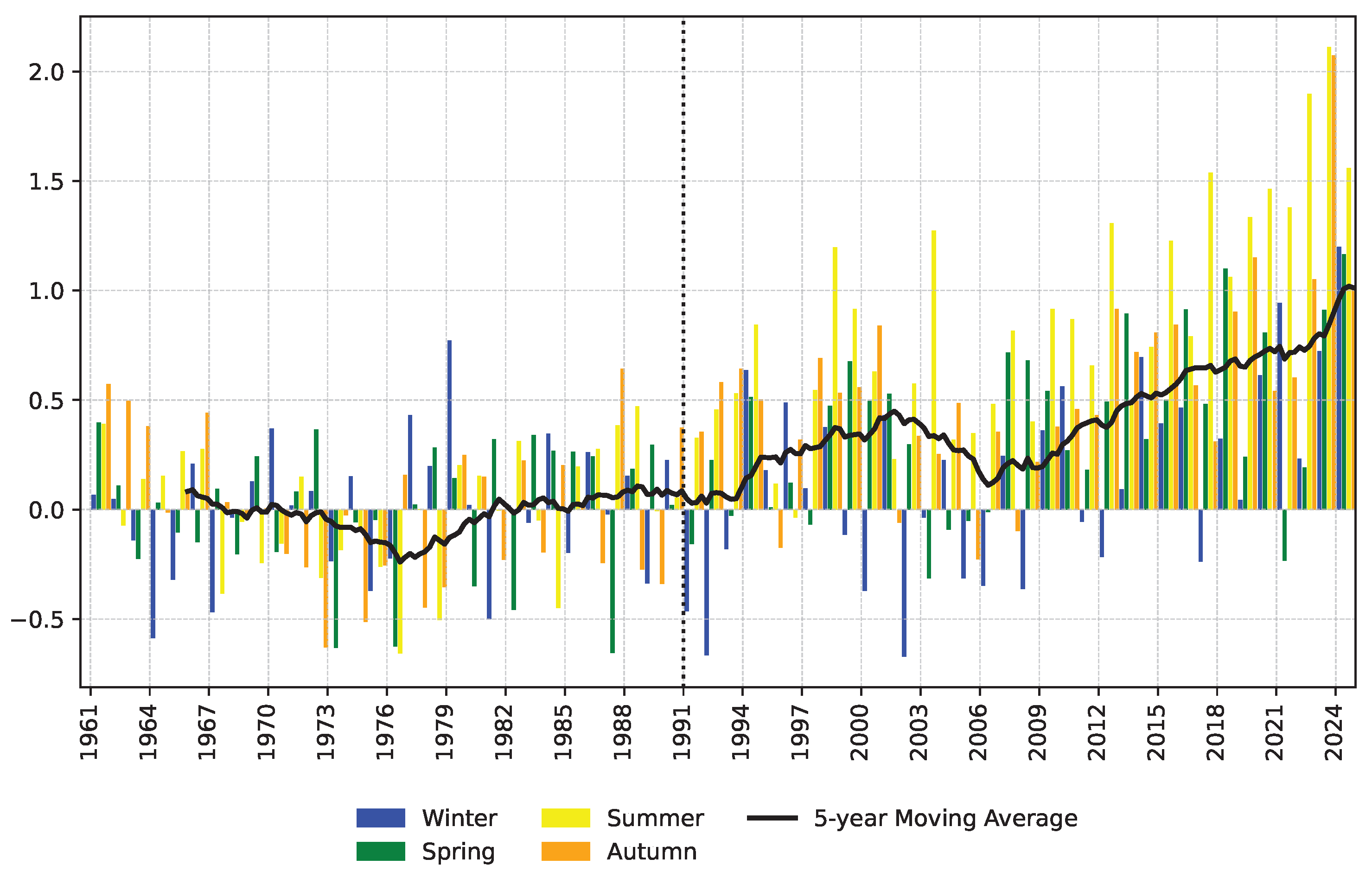
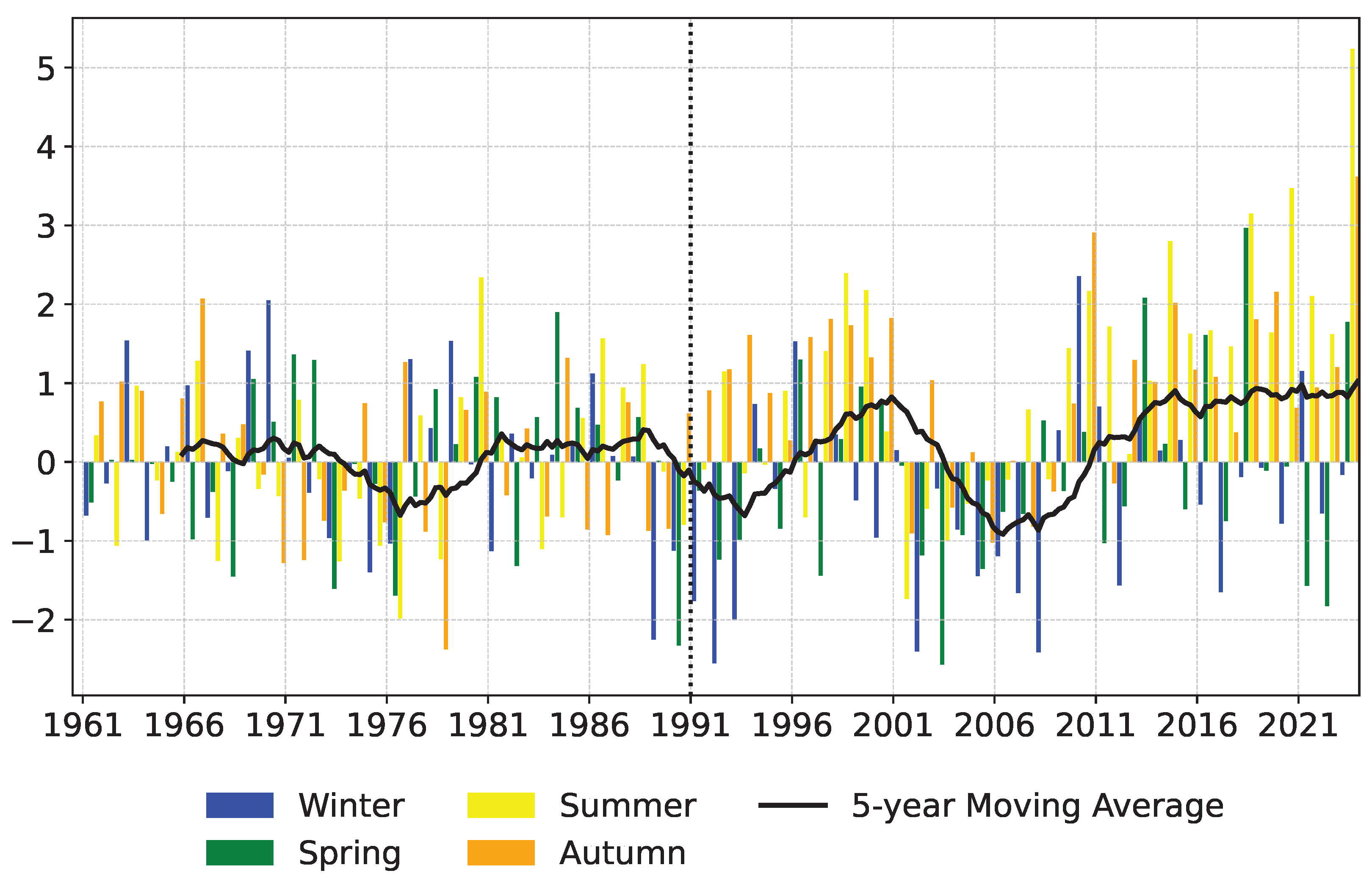
The ITACI is computed by fully incorporating the sea level component (see Equation (1), with w S I = 1 ), in line with the methodological framework described in Section 4. Figure 4 shows the seasonal values together with the five-year moving average, revealing a consistent upward trend over the past two decades.
The 5-year moving average, shown as a black curve in Figure 4, illustrates the long-term evolution of the national ITACI by smoothing short-term seasonal fluctuations. During the reference period, the curve remains close to zero, with no significant deviations, dipping below it for about a decade. This suggests a limited incidence of persistent climatic anomalies at the national scale, particularly given that these years constitute the climatological baseline. A sustained and consistent increase becomes apparent from the mid-1990s, with values steadily rising above zero. The upward trend was briefly interrupted between 2001 and 2006 by a temporary decline, after which the curve resumed its ascent, accelerating over the most recent decade and eventually reaching the highest levels on record. The persistence of these elevated values indicates that seasonal climate anomalies, once sporadic, have become a structural and increasingly defining feature of the Italian climate profile. Short-term factors, such as sea level variability (as discussed in the following section), may occasionally introduce temporary reversals within this overarching upward trend.
Summer consistently records the highest values, with several extreme peaks. This pattern likely reflects the intensification of heatwaves and other summer-specific climate-related extremes observed in recent decades. Spring and autumn both show an upward trend, although their peaks appear less regular over time. These fluctuations may be linked to more episodic climatic phenomena, such as intense rainfall events or temperature anomalies. Winter frequently records negative values before 2009, whereas only three are observed in the subsequent years, suggesting a shift from year-to-year variability to a more moderate and stable regime.
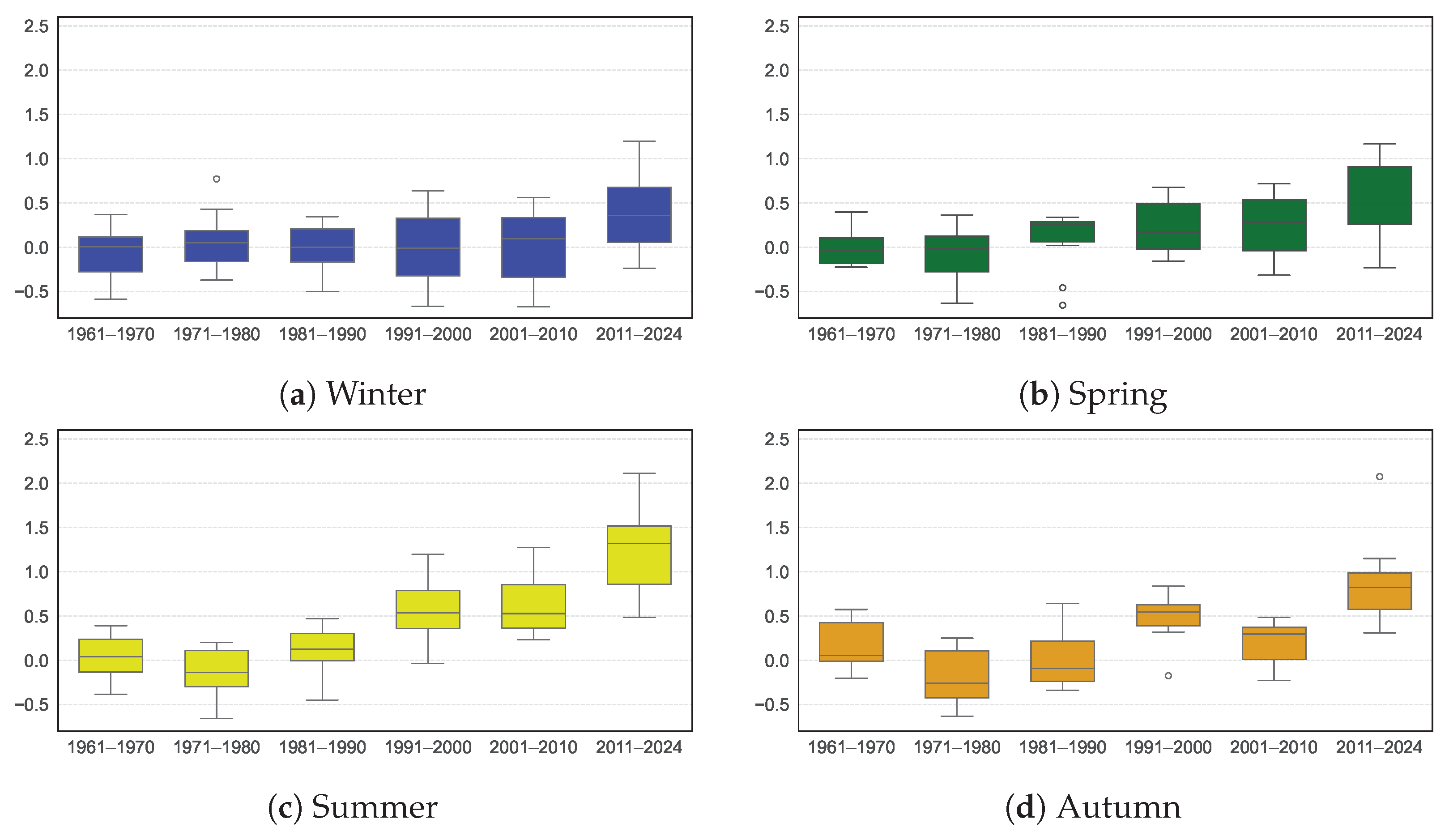
The boxplots in Figure 5 provide a complementary view of seasonal dynamics, highlighting structural changes in ITACI distributions across six time intervals from 1961 to 2024. For summer and autumn, a clear upward shift in the median emerges in 1991–2000, whereas spring and winter show delayed increases beginning after 2000.
The interquartile range (IQR) expands over time, reflecting broader shifts in the seasonal distribution of ITACI values. In summer, the IQR widens steadily in the last two intervals, with the median approaching the upper quartile, indicating that heightened climate-related stress has become structurally embedded in the season rather than being the result of isolated extremes. Spring exhibits a similar widening of the IQR, although the median remains closer to the lower quartile, suggesting a more balanced distribution. Nonetheless, elevated ITACI values are no longer sporadic in spring, reinforcing the notion of a progressively altered seasonal regime. In autumn, the IQR expands moderately, and the median shifts from a lower to a higher position within the box, suggesting that higher values have become more frequent and increasingly dominant in the seasonal distribution. In winter, a notable widening of the IQR is observed in the last three intervals, consistent with the transition noted earlier from a frequent occurrence of negative values to a regime characterised by predominantly positive seasonal values.
In the most recent periods, all seasonal values remain within the statistical whiskers, suggesting that the intensification of ITACI is not driven by isolated extremes but by a systematic upward shift in the underlying distribution.
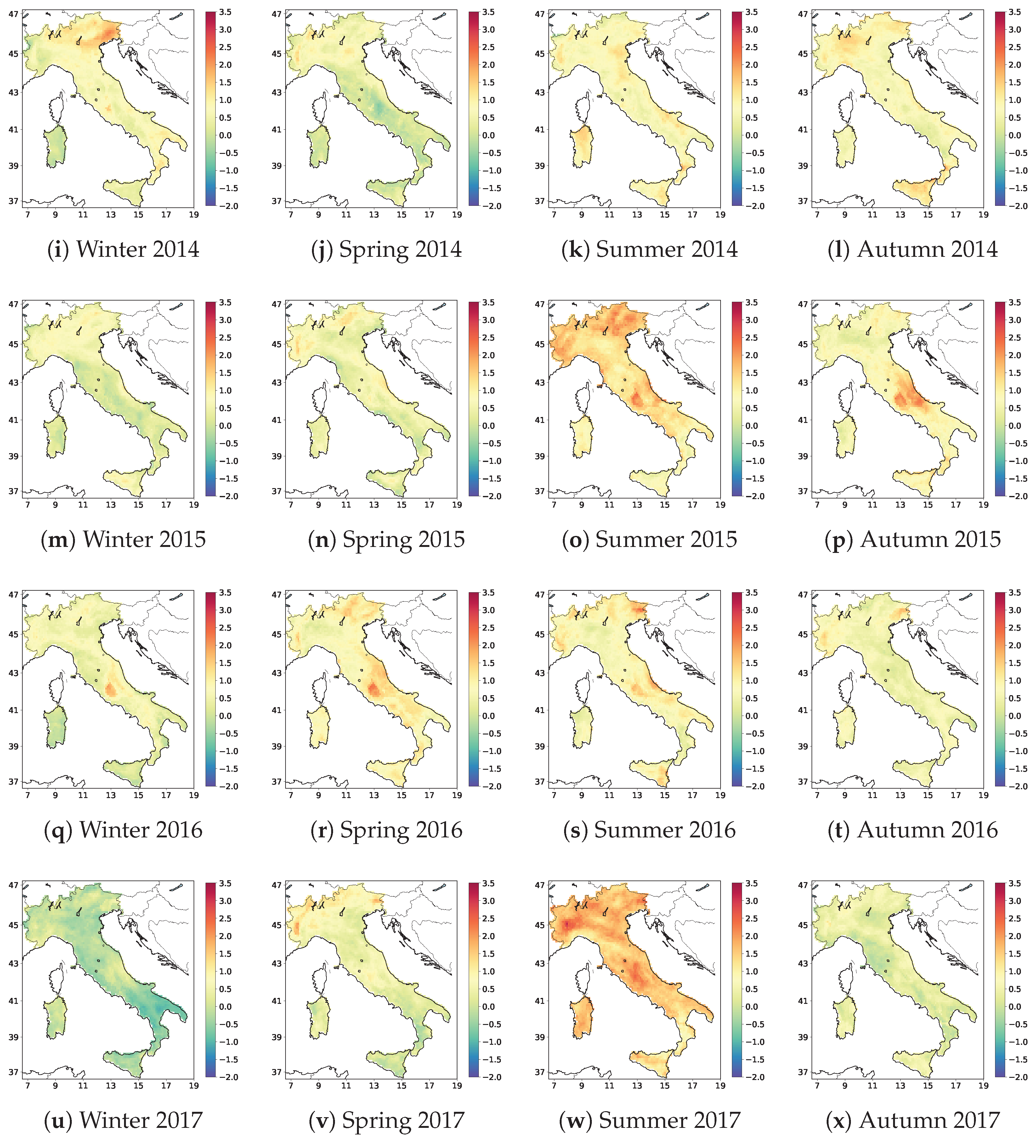
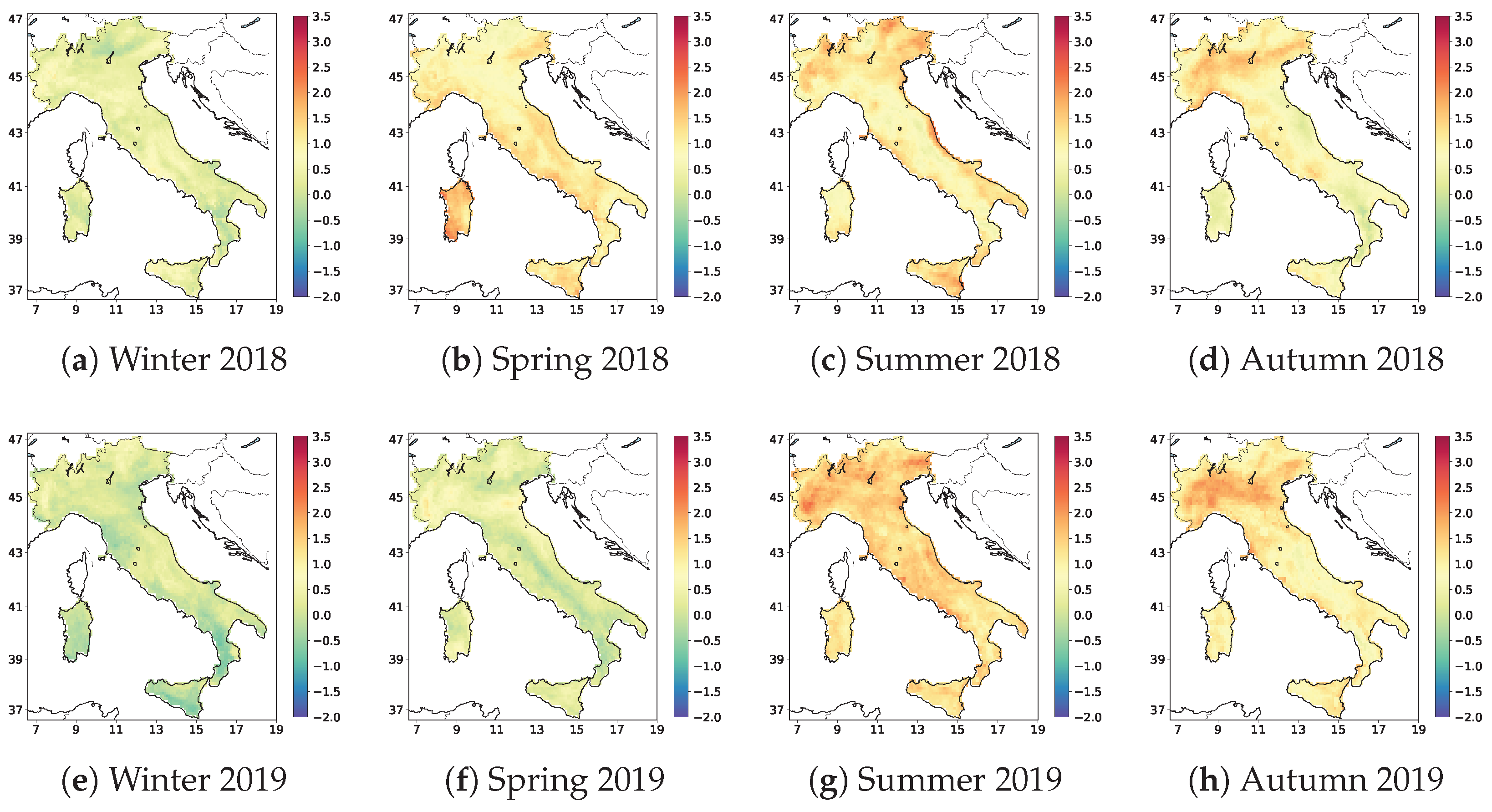
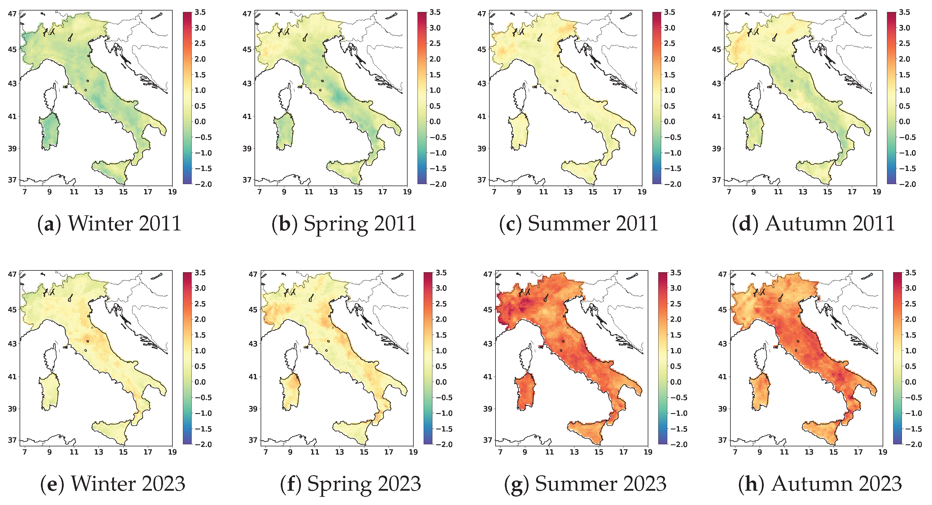
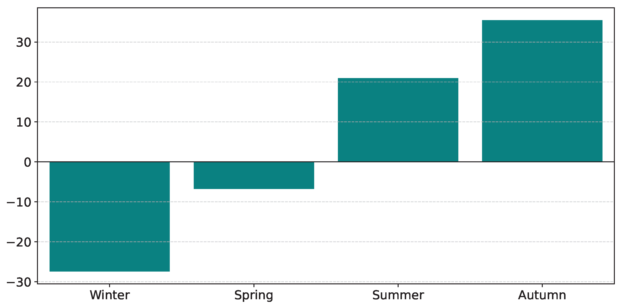
Figure 6 presents the spatial distribution of the seasonal ITACI at high resolution for the years 2011 and 2023. A clear shift towards more intense and spatially coherent seasonal climate stress patterns is observed, indicating a transition to a more widespread and persistent climatic stress regime, with summer and autumn displaying the most extensive and consistent signals. In these two seasons, 2023 is characterised by both broader spatial coverage and higher intensity values. The complete set of maps for all years from 2012 to 2022 is provided in Appendix A.

5.2. ITACI Patterns Across Italian Macro-Regions

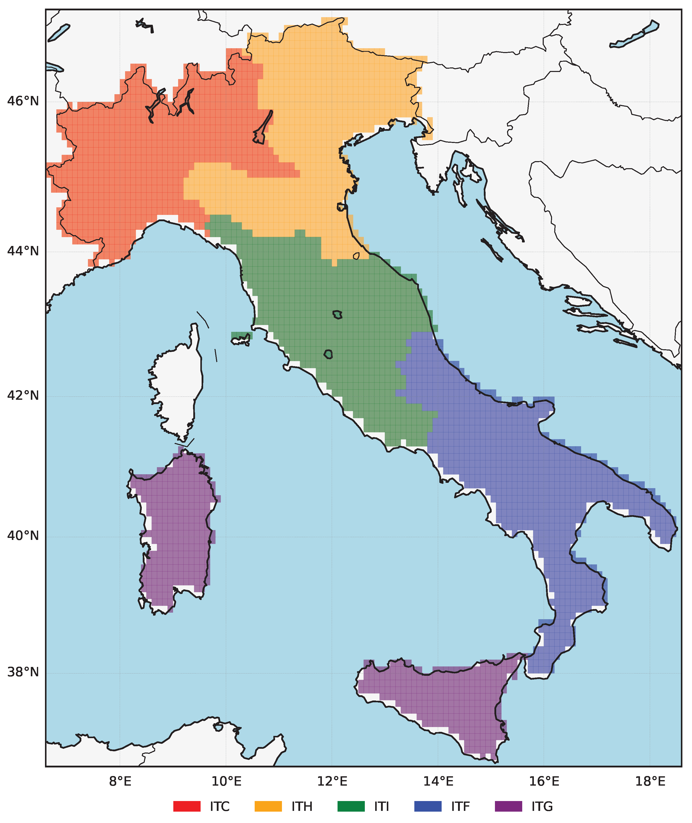
To capture regional differences in climate-related stress, the ITACI is computed separately for five macro-areas, corresponding to the NUTS1 classification (see Table 2). Figure 7 presents the spatial delineation of the five macro-areas, with each 0.1° grid cell assigned to a specific NUTS1 region.
As the five macro-areas satisfy properties (4), Formula (6) holds with K = 5 , and α k is computed using the values of N k reported in Table 2. The sea-level weights w S A k are defined as the ratio between the coastline length of each macro-area and the national total, thereby accounting for differential exposure to sea level variability. For instance, the Islands represent nearly 45% of the national coastline but only 15% of the climate indicator grid cells, whereas the North-West accounts for less than 5% of the coastline and about 21% of the grid cells.
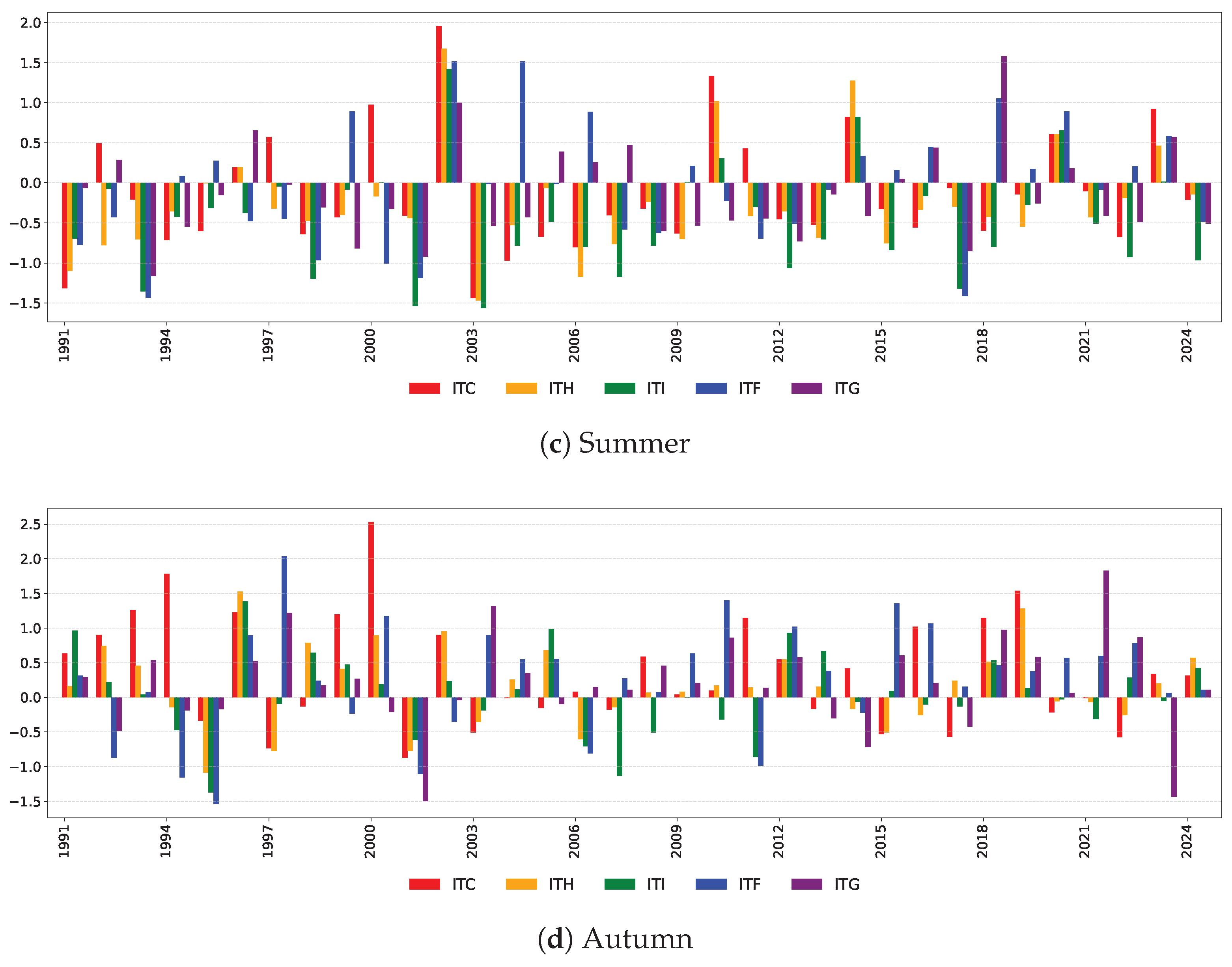
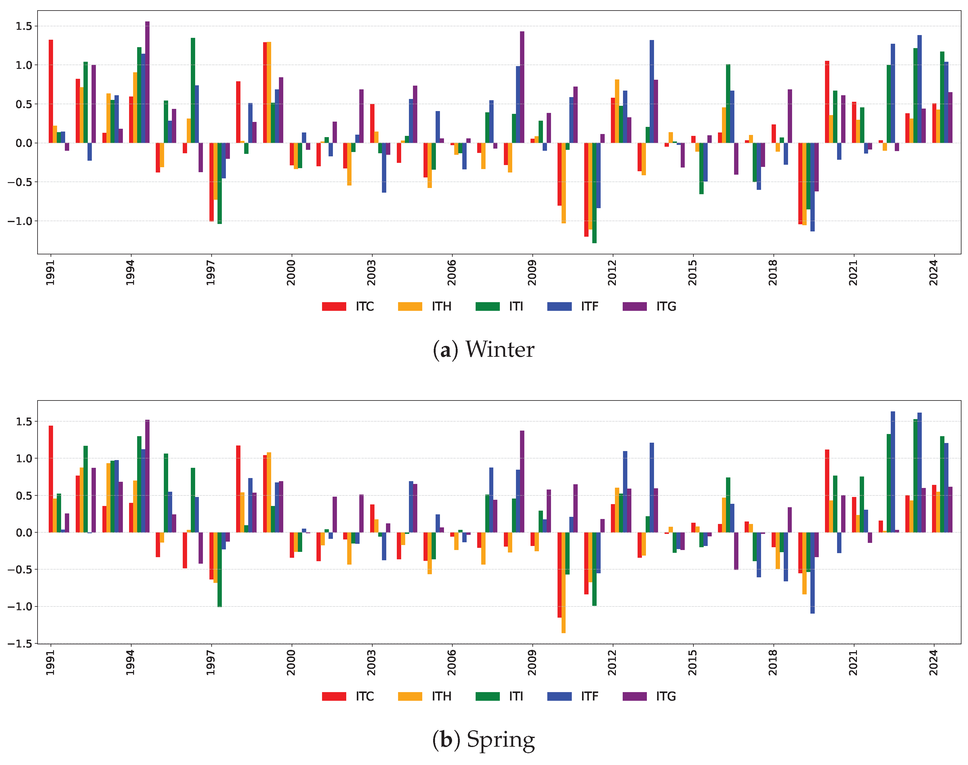
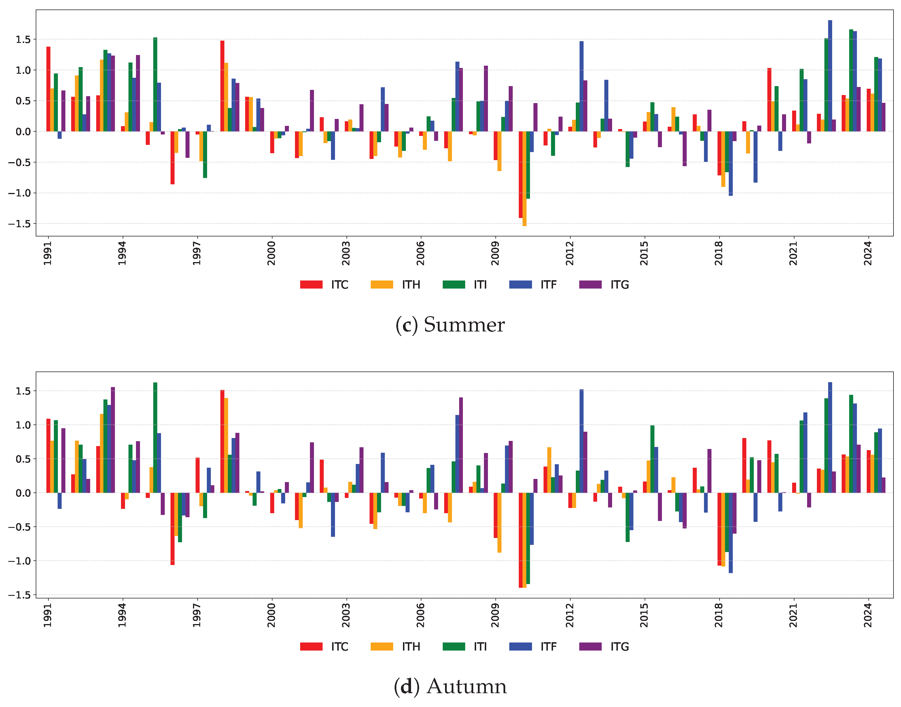
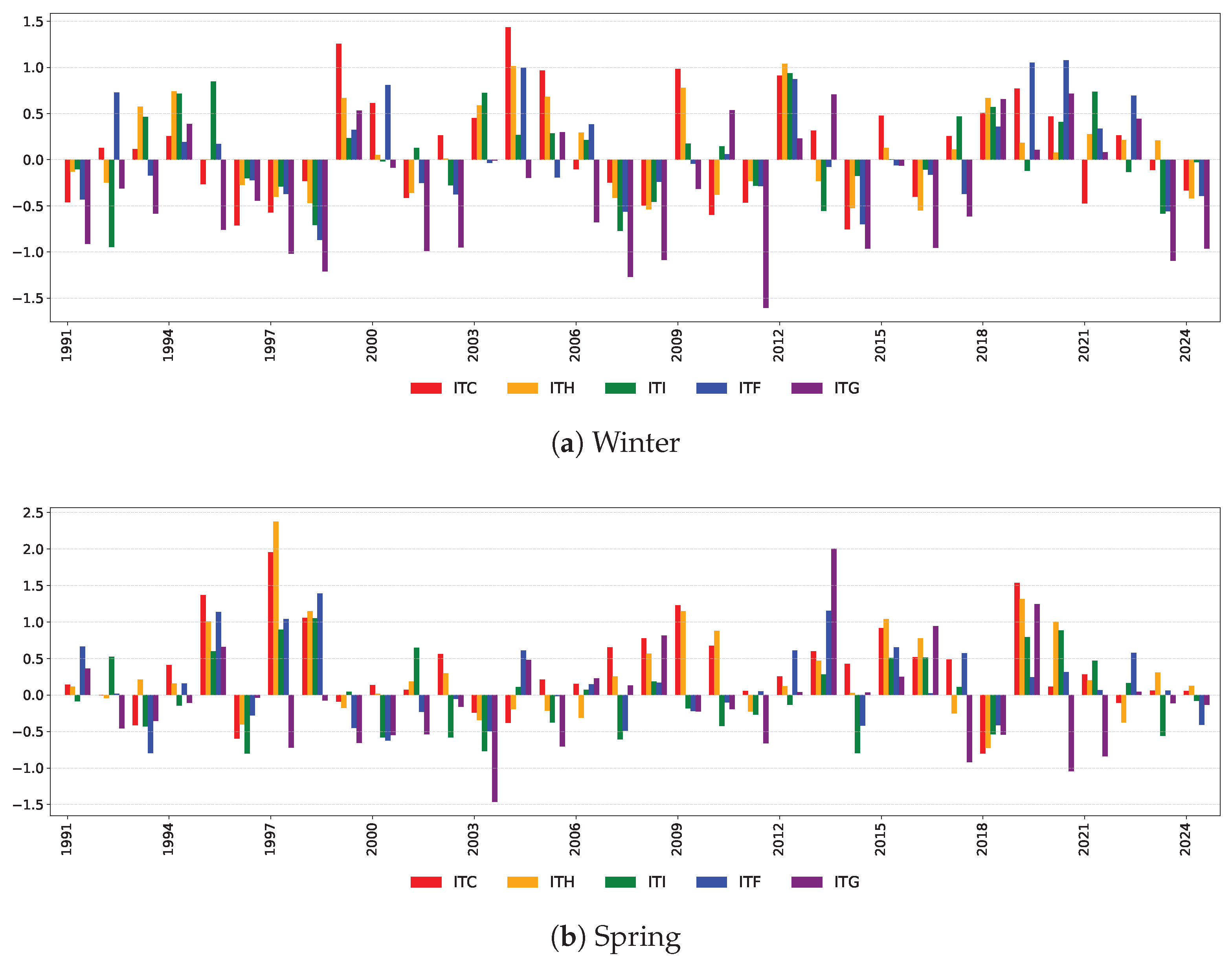
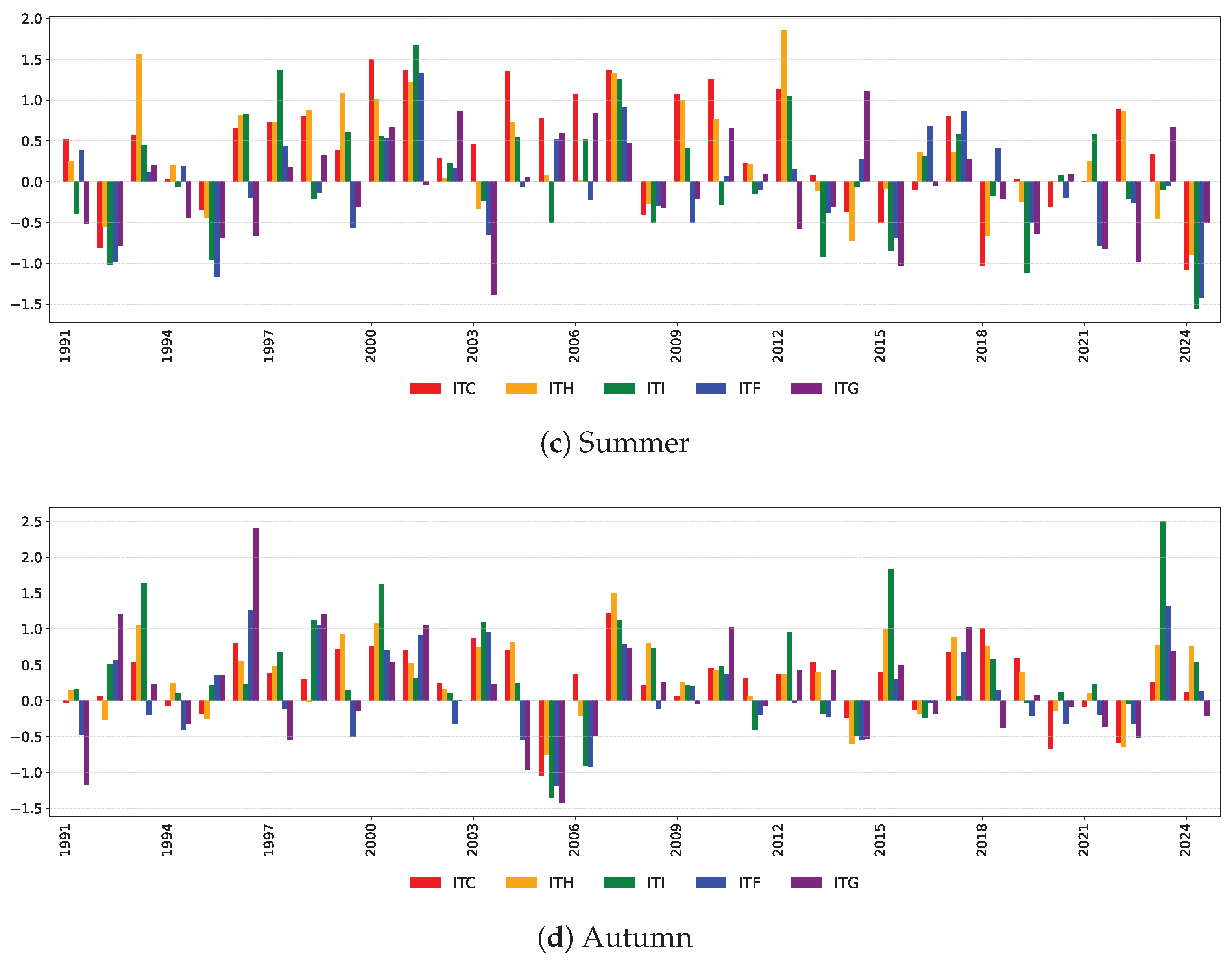
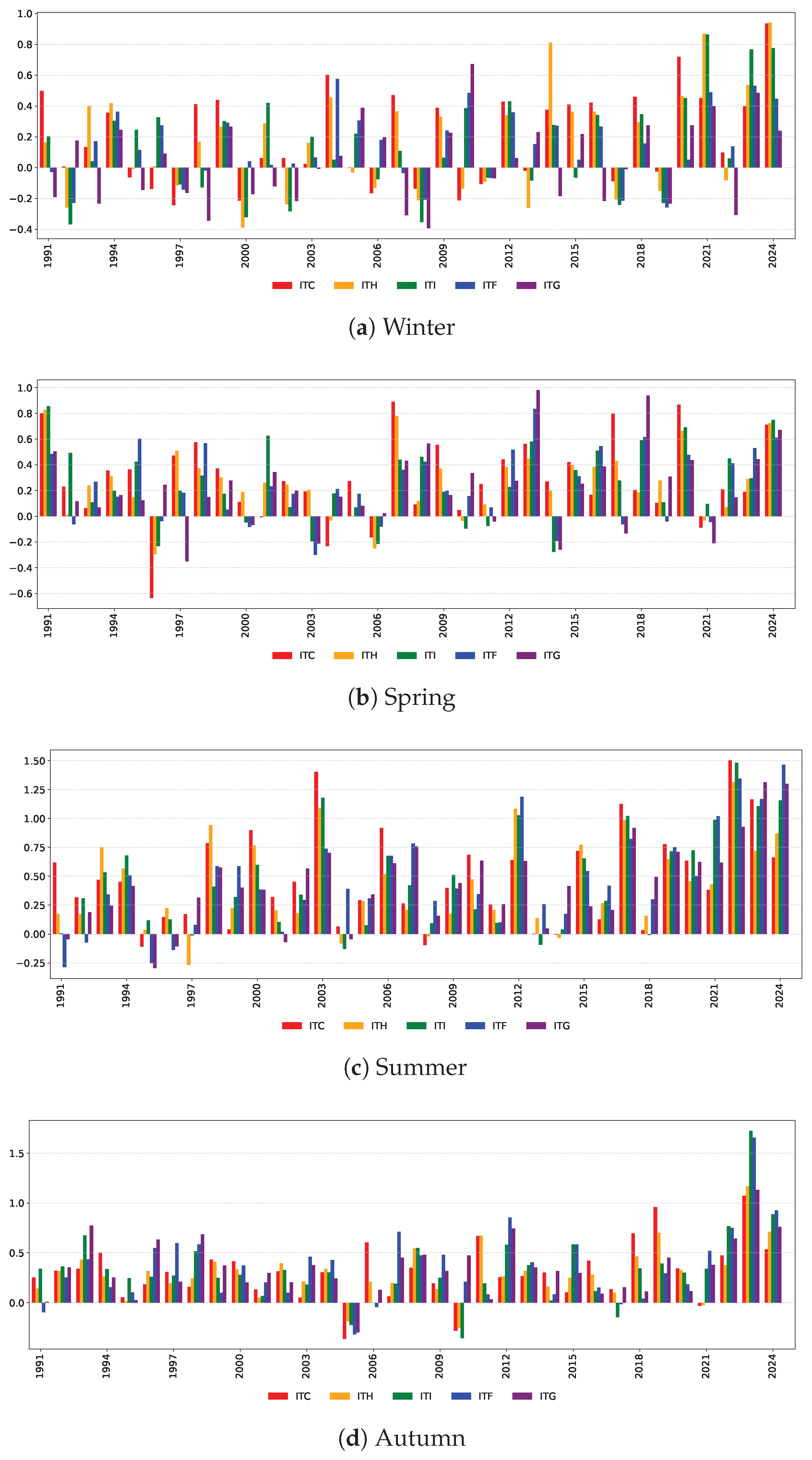
Figure 8 shows the seasonal ITACI values by macro-area. As 1961–1990 serves as the climatological baseline, the analysis focuses on the period from 1991 onwards, where standardised anomalies effectively capture deviations from historical norms attributable to climate change.
The cold season shows a marked intensification of climate-related stress in northern and central Italy, as evidenced by the rise in subnational ITACI values since the early 2000s (Figure 8a). The northern (ITC and ITH) and central (ITI) regions have recorded the highest levels in recent years. As the sea level component contributes relatively little to these regions, the observed increases are likely driven mainly by changes in atmospheric indicators.
Spring ITACI values exhibit a clear and gradual intensification of climate stress across all macro-areas (Figure 8b). Early in the observed period, significant signals emerge mainly in the northern and central macro-areas (ITC, ITH, ITI). From 2007 onwards, positive anomalies became more frequent nationwide, accompanied by a steady decline in negative values. The southern and island macro-areas (ITF and ITG) show the most consistent and sustained increases, while the northern and central regions enter a renewed growth phase beginning around 2018. Overall, this pattern reflects a progressive expansion and strengthening of spring climate stress throughout the country, with the southern and island areas demonstrating the most pronounced and persistent changes.
Summer shows the most uniform and persistent increase in ITACI values among all seasons, with values exceeding +1 in every region (Figure 8c). The Islands (ITG), the South (ITF), and the Centre (ITI) display particularly strong signals, while the northern regions (ITC and ITH) have often reached comparable levels in recent decades. Regional differences tend to narrow in recent years, suggesting a process of climate convergence, whereby all macro-areas are increasingly exposed to similar levels of seasonal climate stress. Summer thus emerges as the clearest seasonal expression of systemic climate stress in Italy.
Autumn exhibits predominantly positive ITACI values across all macro-areas, reflecting structurally altered climate patterns nationwide (Figure 8d). The southern (ITF) and island (ITG) macro-areas record the most significant increases, while the North-West (ITC) shows a slower response. In the most recent period, all macro-areas consistently display elevated values (see also Figure 6h).
In conclusion, northern and central Italy have experienced the most pronounced shift in winter, likely because the South and Islands are climatically distinct, with persistent impacts emerging mainly during spring and autumn. The summer season reveals a strong and uniform climate change signal across all macro-areas.
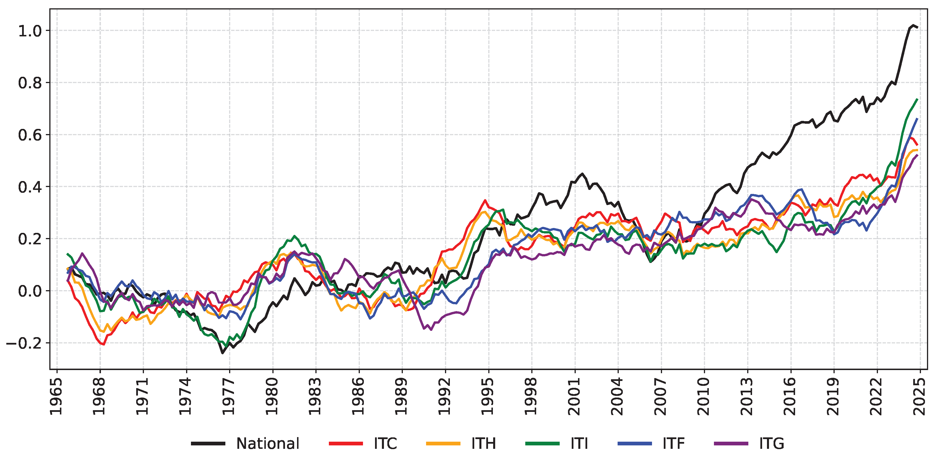
To complete the seasonal analysis, Figure 9 shows the five-year moving average ITACI trajectories at both national and macro-area levels. No single macro-area consistently dominates the others over time, with some even exhibiting opposing trends during different subperiods. This lack of synchrony is likely attributable to geographical, meteorological, and environmental factors, as well as regional influences such as microclimates or temporary phenomena. The contribution of sea level is significant in the most exposed areas, as will be discussed later. Each macro-area contributes to the national ITACI trajectory proportionally to spatial aggregation weights based on the number of grid cells and exposure weights related to sea level vulnerability (see Formula (5) and Table 2). The Centre (ITI) and Islands (ITG) play a key role in the marine component, whereas the northern areas, which are spatially larger but less exposed to marine influence, contribute primarily through the atmospheric component to the national climate index.

5.3. Drivers of ITACI Dynamics: Indicator-Level Analysis

This subsection analyses seasonal trends of individual atmospheric indicators to identify and explain the main drivers of the evolving climate-related stress in Italy. The analysis of sea level is presented in Section 6.3.
  • National Analysis
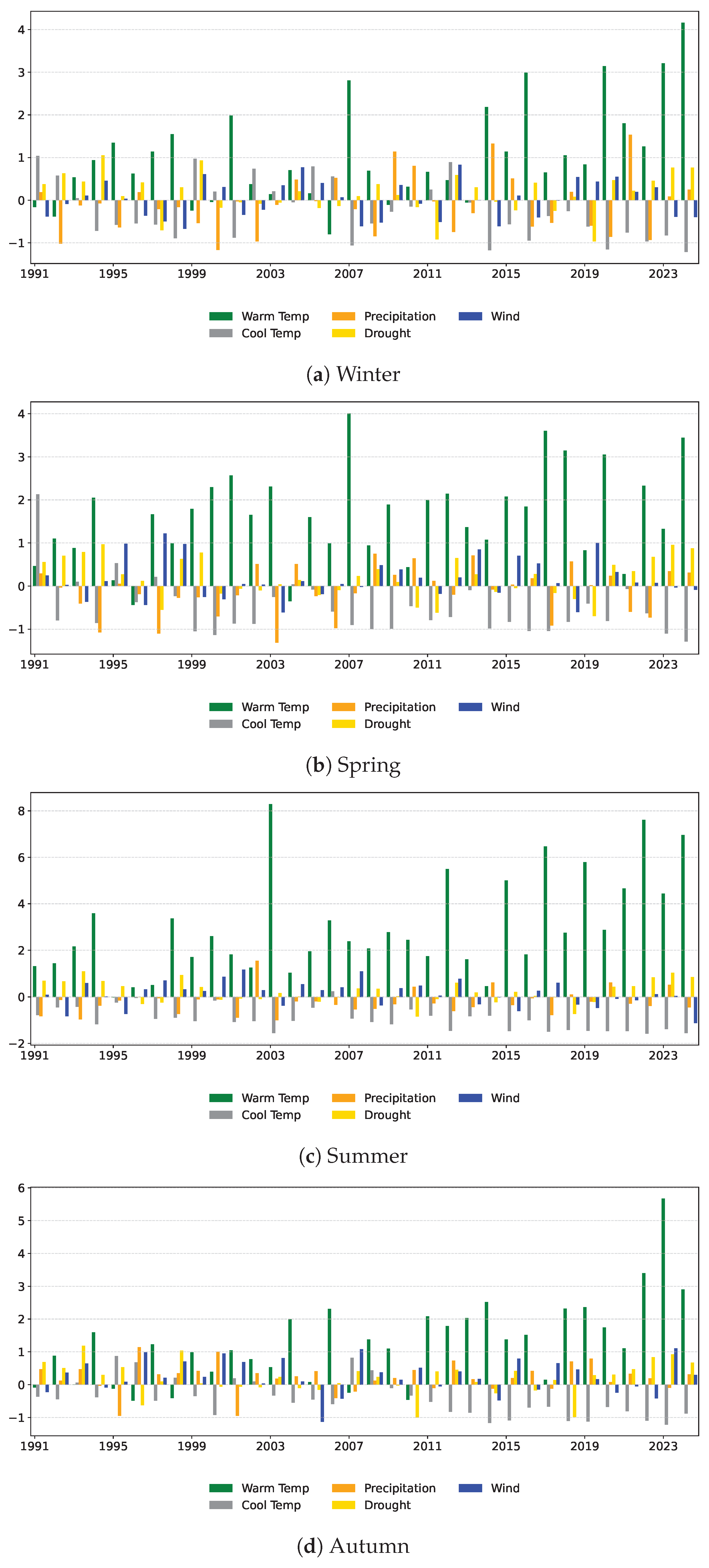
Figure 10 shows the standardised anomalies of the atmospheric indicators at the national level for each season.
The analysis reveals a progressive reshaping of seasonal climate dynamics in Italy over the period 1991–2024, with each season exhibiting distinct yet interconnected shifts. Summer emerges as the most profoundly transformed season, characterised by persistent and intensifying heat stress alongside the systematic disappearance of day- and night-time cold extremes. Moreover, a persistent combination of positive Drought anomalies and negative Precipitation values indicates a structural transition towards recurrent water shortages (Figure 10c). Spring reveals an early onset of warmth, with Cold Temperature anomalies consistently below zero over the past two decades and Warm Temperature anomalies intensifying since the 2000s. Although more moderate than in summer, Drought anomalies have become structurally positive in recent years, while five-day cumulative precipitation remains erratic, indicating mounting hydrological instability (Figure 10b). Autumn in Italy is also shifting towards a later and warmer seasonal transition, with prolonged periods of water scarcity accompanied by an increase in rainfall concentrated in a few intense episodes (Figure 10d). Winter, though still the most variable season, shows a persistent thermal shift towards milder conditions: Cold Temperature anomalies have been consistently negative since 2014, while Warm Temperature anomalies have intensified sharply. The hydrological profile reveals that Drought and Precipitation anomalies are increasingly decoupled, resulting in a more complex and less predictable hydrological regime (Figure 10a).
Wind Power anomalies exhibit a modest and discontinuous signal across all seasons. In winter and spring, moderate interannual variability is observed, with no sustained trend over the period. Several winters (1999, 2004, 2012, and 2020) record notable positive anomalies, while spring shows isolated peaks (1995, 1997, 1998, 2013, and 2019). However, these episodes remain sporadic and insufficient to indicate structural change. Summer displays the weakest and most erratic signal, with moderate positive values in 2000, 2001, 2007, and 2012, but no coherent temporal pattern. Even in autumn, where the seasonal mean during the calculation period reaches a slightly elevated value (+0.26), year-to-year variability dominates, and no sustained increase is detected. Overall, Wind Power contributes minimally to the national ITACI, reflecting mainly short-term atmospheric variability rather than long-term climatic trends.
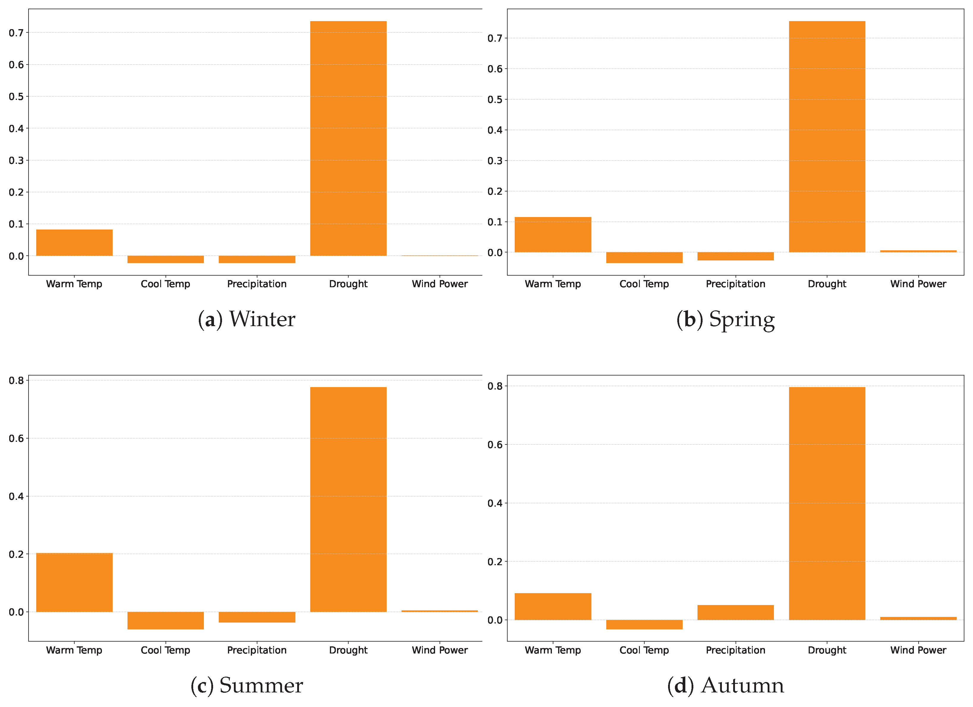
Figure 11 confirms the previous analysis by displaying the mean (non-standardised) anomalies for each season6. The increase in the frequency of warm extremes and the decrease in cold extremes affect all seasons, with the most pronounced changes occurring in summer. The length of drought periods affects all seasons to a similar extent. Five-day cumulative precipitation shows an increase only in autumn. Wind Power contributes only marginally to mean seasonal anomalies, as values across all seasons remain close to zero with no appreciable deviation.
Figure 12, which displays the correlation coefficients between ITACI and its six components based on monthly values, shows that the composite signal is only moderately influenced by the atmospheric indicators, with the exception of cool temperature, whose contribution is markedly weaker.
The strong negative correlation (−0.52) between warm and cool temperatures is expected, given their complementary definitions. The negative correlation between warm temperature and precipitation (−0.26) suggests a climatological link, whereby hot extremes tend to coincide with reduced five-day cumulative rainfall. The weak positive correlation with drought (+0.17) appears surprisingly low, given the potential link between heat extremes and prolonged dry periods. While high temperatures and drought conditions often co-occur during summer, in other seasons warm anomalies may arise without a corresponding increase in dry spell duration, thereby weakening the overall monthly correlation. Finally, the moderate positive correlation between wind power and cool temperature (+0.35), combined with its weak negative correlation with warm temperature (−0.16), suggests that wind activity tends to intensify during cooler conditions and diminish during heat extremes.
  • Regional Analisys
The analysis is structured by season and draws on five figures presented in Appendix B, from Figure A3, Figure A4, Figure A5, Figure A6 and Figure A7, each displaying the standardised anomalies associated with the respective atmospheric indicator.
The North-West (ITC) exhibits some of the earliest climate signals in the country, particularly the attenuation of cold extremes during winter and spring. Initially moderate, positive temperature anomalies have become increasingly frequent and intense over the last two decades, with a clear summer intensification. In hydrological terms, the area shows a weakening in the intensity of five-day cumulative precipitation events, especially during winter and spring. Drought anomalies occur irregularly, without a sustained trend.
The North-East (ITH) follows a similar trajectory, though with greater variability. Cold extremes have declined significantly since the early 2000s, while warm anomalies have intensified erratically, with notable peaks. Hydrological behaviour is the most volatile among all macro-areas: the intensity of five-day precipitation events fluctuates markedly across years, alternating between accentuated and attenuated phases. Summer also reveals increasing instability in precipitation dynamics.
Central Italy (ITI) displays the most coherent and persistent climate shift. All seasons show a steady increase in warm anomalies and a clear reduction in cold extremes, while drought conditions have become structural. The maximum intensity of five-day precipitation events tends to decline, particularly in summer.
Southern Italy (ITF) follows a more delayed trajectory but has undergone a marked acceleration over the last decade. Winters and springs are increasingly affected by warm anomalies, while summers record extreme peaks. Hydrological stress is also rising, with recurring drought anomalies and a reduction in seasonal precipitation maxima.
The Islands (ITG) reveal a similarly delayed but now evident shift: warm anomalies are gradually intensifying, particularly in summer and autumn, while cold extremes decline more slowly but consistently. Chronic drought conditions now characterise the region, accompanied by a downward trend in the maximum intensity of five-day precipitation events. Wind signals appear weak or declining.
Overall, these regional trajectories confirm a progressive warming and growing hydrological instability, with dynamics differing in timing, magnitude, and spatial coherence.
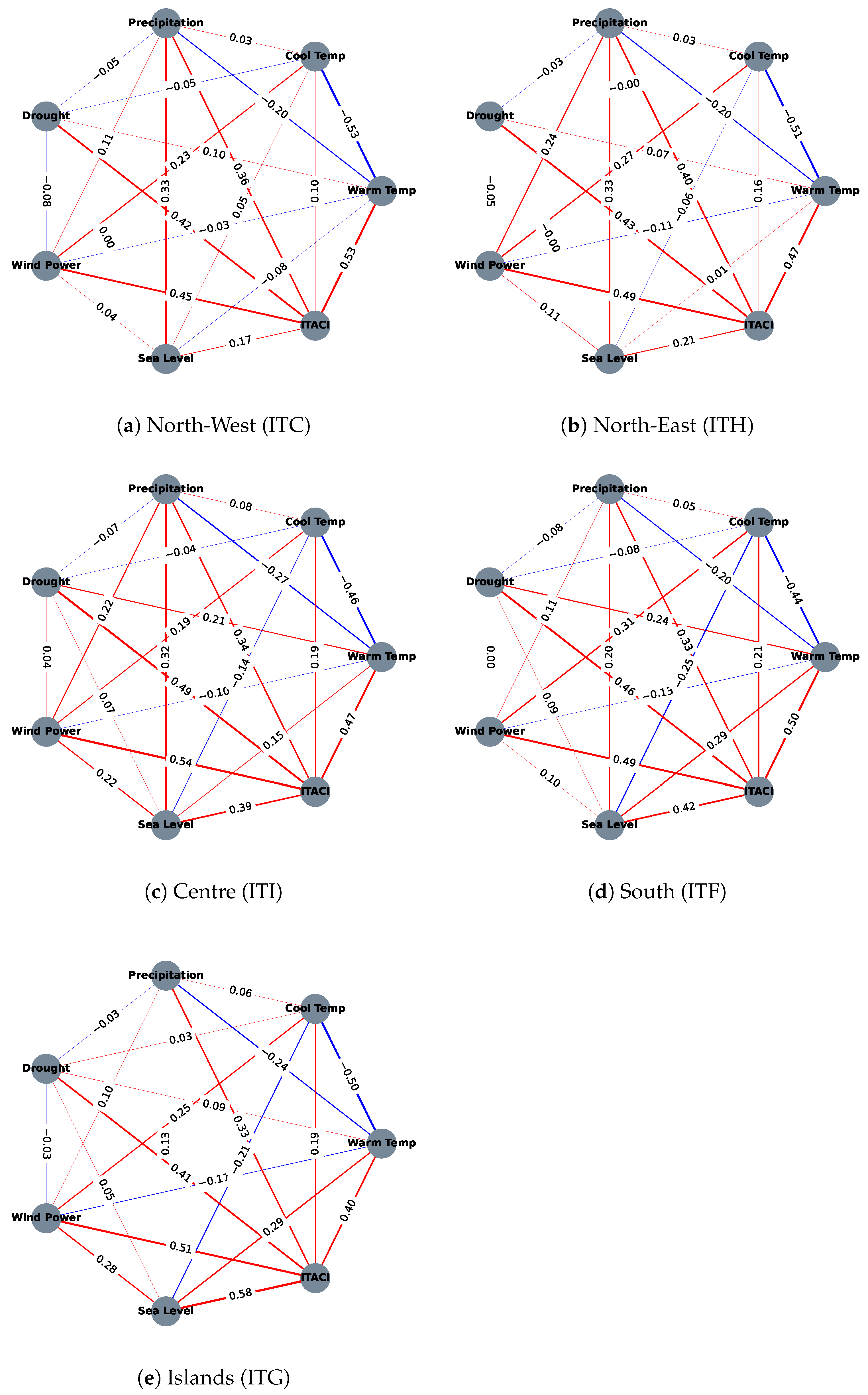
Figure 13 presents the correlation coefficients for each macro-area. Among the atmospheric indicators, warm temperature emerges as the primary driver of the aggregated index, with the North-West (ITC) showing the strongest influence and the Islands the weakest. Cool temperature displays a positive correlation across all macro-areas, with Southern Italy (ITF) exhibiting approximately twice the correlation of the North-West (ITC), corroborating previous findings. Hydrological indicators display similar correlation values across regions, indicating a broadly uniform influence across the territory. The wind component follows the same pattern, with the Centre (ITI) showing the strongest influence.

6. Comparative Analysis with European Indices

National correlation coefficients differ from regional ones and can sometimes show opposite behaviour because aggregating opposing local anomalies tends to cancel them out (see Figure 12 and Figure 13). This is evident for cool temperature, where the national correlation is slightly negative (–0.03), whereas for warm temperature and drought, the national correlations are lower (0.39 and 0.27, respectively), showing that aggregation at the national scale can attenuate climate signals that are stronger at the local level. In contrast, the precipitation indicator stands out more clearly at the national level, with a correlation of 0.41, suggesting that the aggregated signal for precipitation is stronger and more coherent when considered across the entire country. This underscores the importance of analysing climate indicators at multiple spatial scales, as aggregation can obscure significant regional heterogeneity.
To place the ITACI in a broader European context, this section compares Italian climate stress dynamics with those captured by the French (FACI) and Iberian (IACI) indices. The common methodological framework highlights national specificities in the climatic signals. The analysis is organised into three parts: the first examines the evolution of the composite index; the second compares individual climate indicators and the third considers sea level trends, which differ markedly in Italy, and therefore, warrant separate discussion. The comparison uses data from Portugal and Spain, while for France it remains qualitative, relying on figures from Garrido et al. (2024)7.

6.1. Cross-Country Trends in the Composite Climate Index

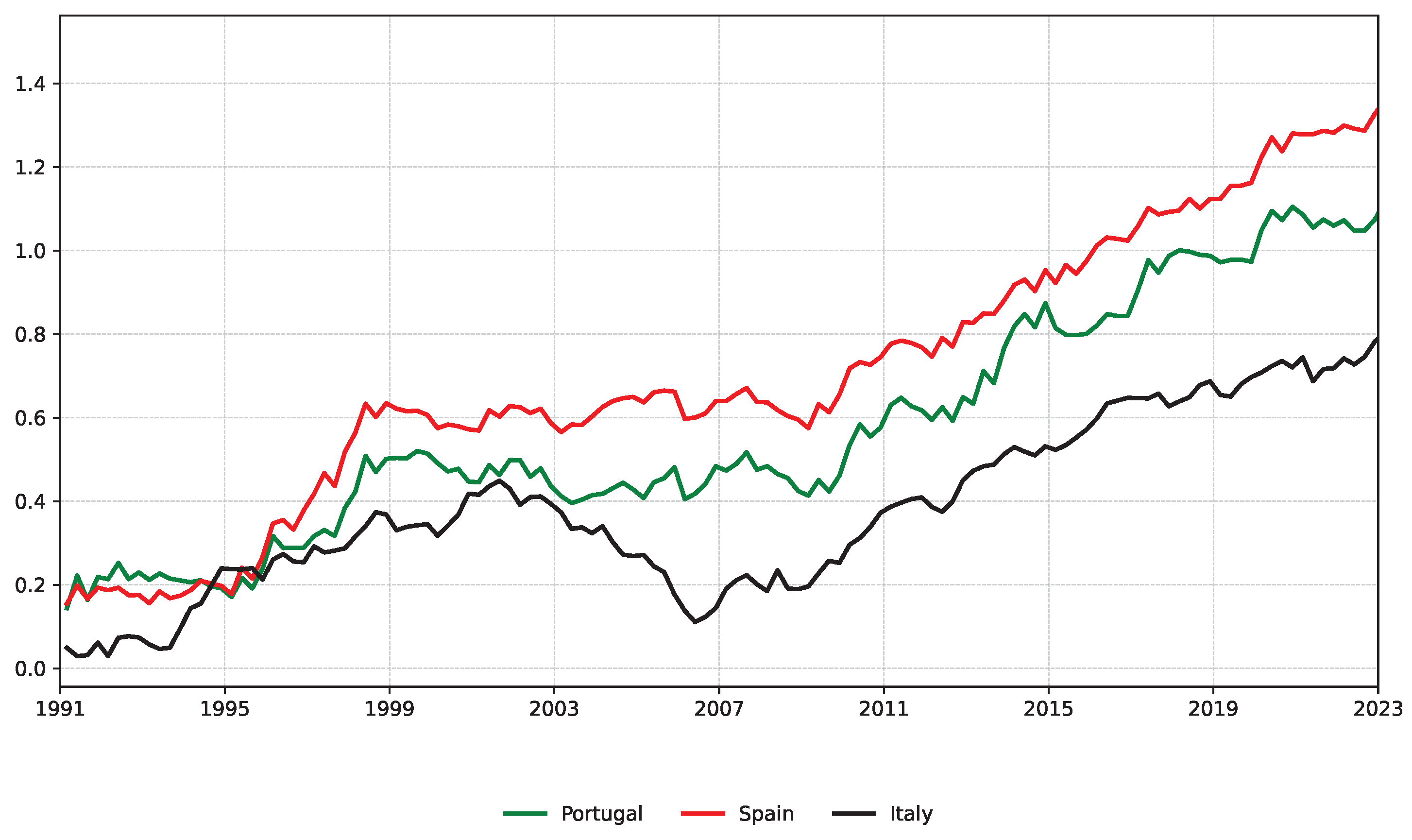
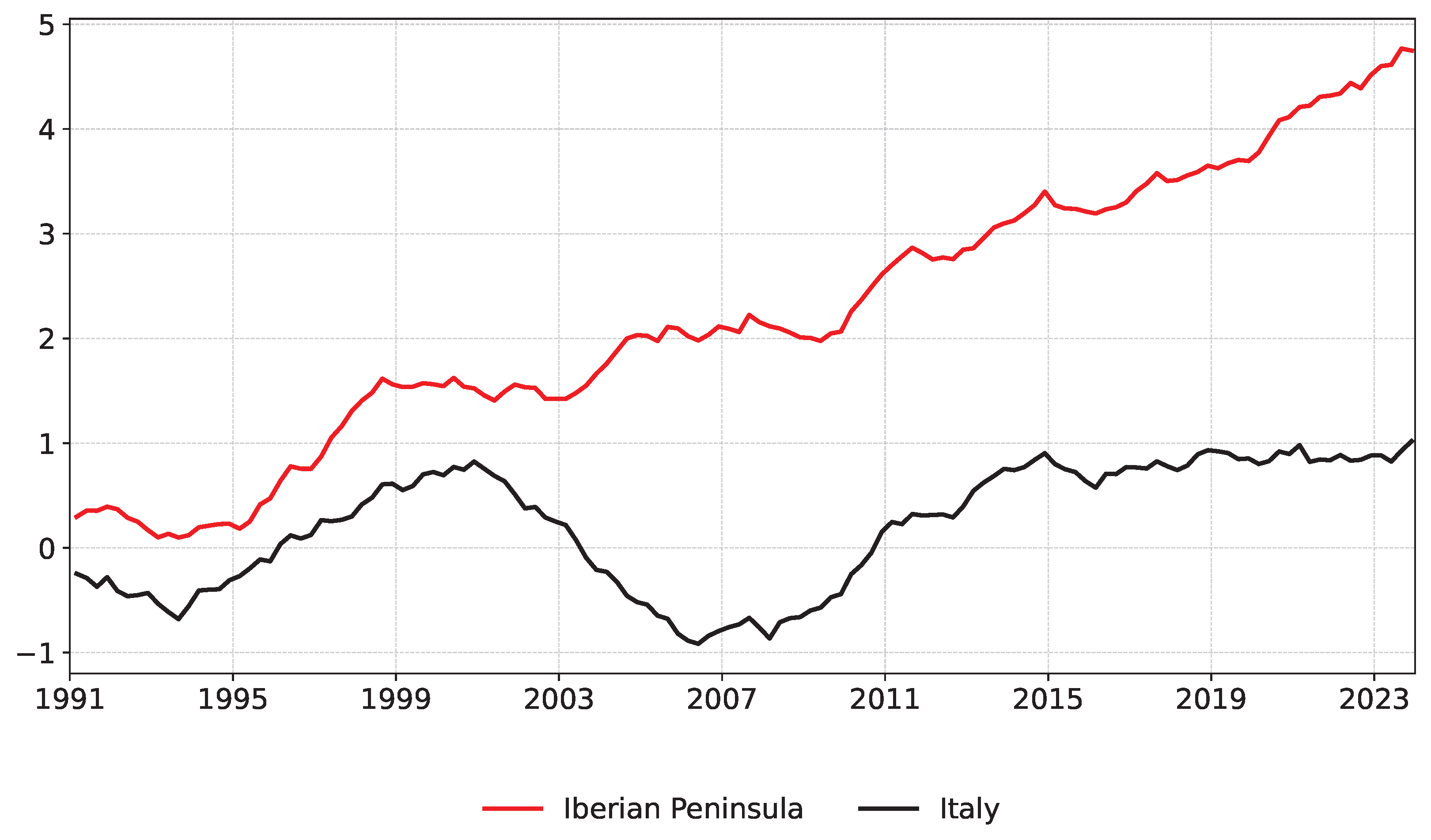
This subsection examines the temporal evolution of the composite index across countries. The comparison assesses whether the Italian trajectory aligns with broader European dynamics or reveals distinct national patterns that may require context-specific risk assessments. Figure 14 shows the five-year moving average for Portugal, Spain, and Italy.
A comparative examination of the composite indices reveals both shared patterns and significant national divergences. After a brief decline in the mid-1990s, the FACI shows two distinct phases of acceleration. The first, in the early 2000s, initiated a gradual upward trend and surpassed +0.6–0.7 by 2003. The second, around 2015, led to values above +1 in 2018–2019 and reached approximately +1.1 in the most recent observations (see Figure 1.4, in Garrido et al. 2024, p. 5).
Over the same period, the Iberian indices show similar trends, with Portugal remaining below the Spanish curve. Both countries experienced earlier accelerations compared with the French index, notably in the mid-1990s and at the end of the 2010s. The gap between the two Iberian indices has widened, increasing from a minimum of 0.08 to a maximum of 0.26, recorded in Winter 2023. The French curve appears to have overtaken the Iberian ones around 2003 and remained close to +0.6 until 2015, when the Iberian indices surpassed it. In recent years, the French and Portuguese curves seem to have converged.
Italy, in contrast, has remained the lowest since the mid-1990s, displaying a distinct pattern. A first upward trend began in 1993, with values increasing markedly from +0.04 to +0.45 by 2001. The Italian index then underwent a prolonged decline from Summer 2002 to Autumn 2008, reaching a low of +0.11 in Spring 2006. Subsequently, a sustained and uninterrupted upward trajectory resumed, carrying the index to +0.90 by the end of the observation period.
Overall, all four countries exhibit clear signs of accelerated climate change, as reflected in the persistent rise of their composite indices. However, Italy stands out for its more fragmented and delayed trajectory, marked by a phase of decline before aligning in the late 2000s with the broader upward trend. These dynamics highlight the importance of nationally constructed climate indicators, such as ITACI, in accurately capturing the specific trajectories of climate-related stress. Such tools are essential for informing differentiated adaptation and mitigation strategies, even within the framework of a coordinated European response.

6.2. Cross-Country Trends in Individual Climate Indicators

This subsection compares the five atmospheric indicators that compose the ITACI with their counterparts in the Iberian and French indices. For Spain and Portugal, the availability of complete time series up to 2023 allows for a detailed analysis of seasonal anomalies and trends. In contrast, the French data are available only in graphical form and are not disaggregated by season. Consequently, the French component of the comparison focuses on general temporal dynamics inferred from the five-year moving average curves.
  • Thermal Indicators: Warm and Cool Temperatures
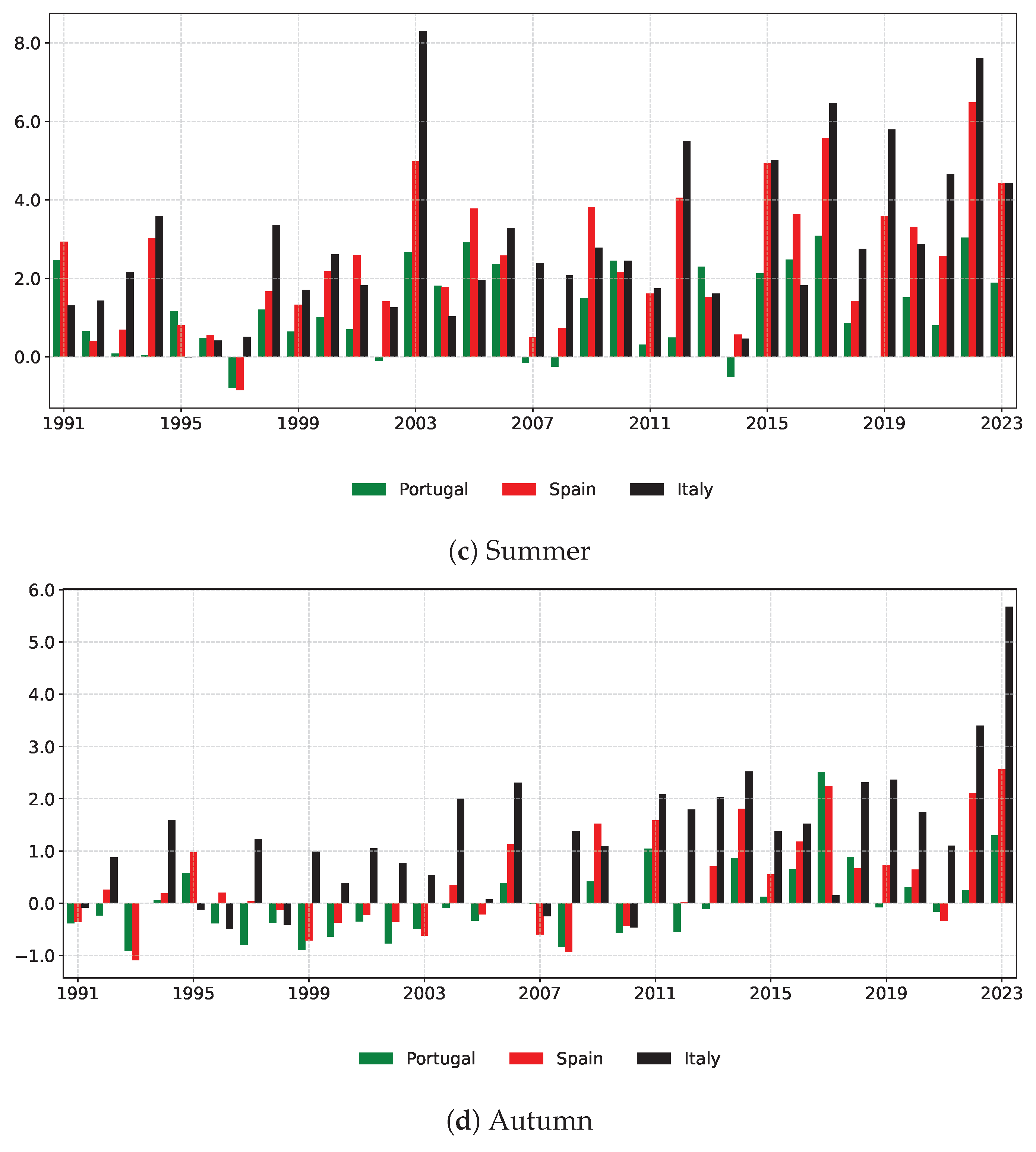
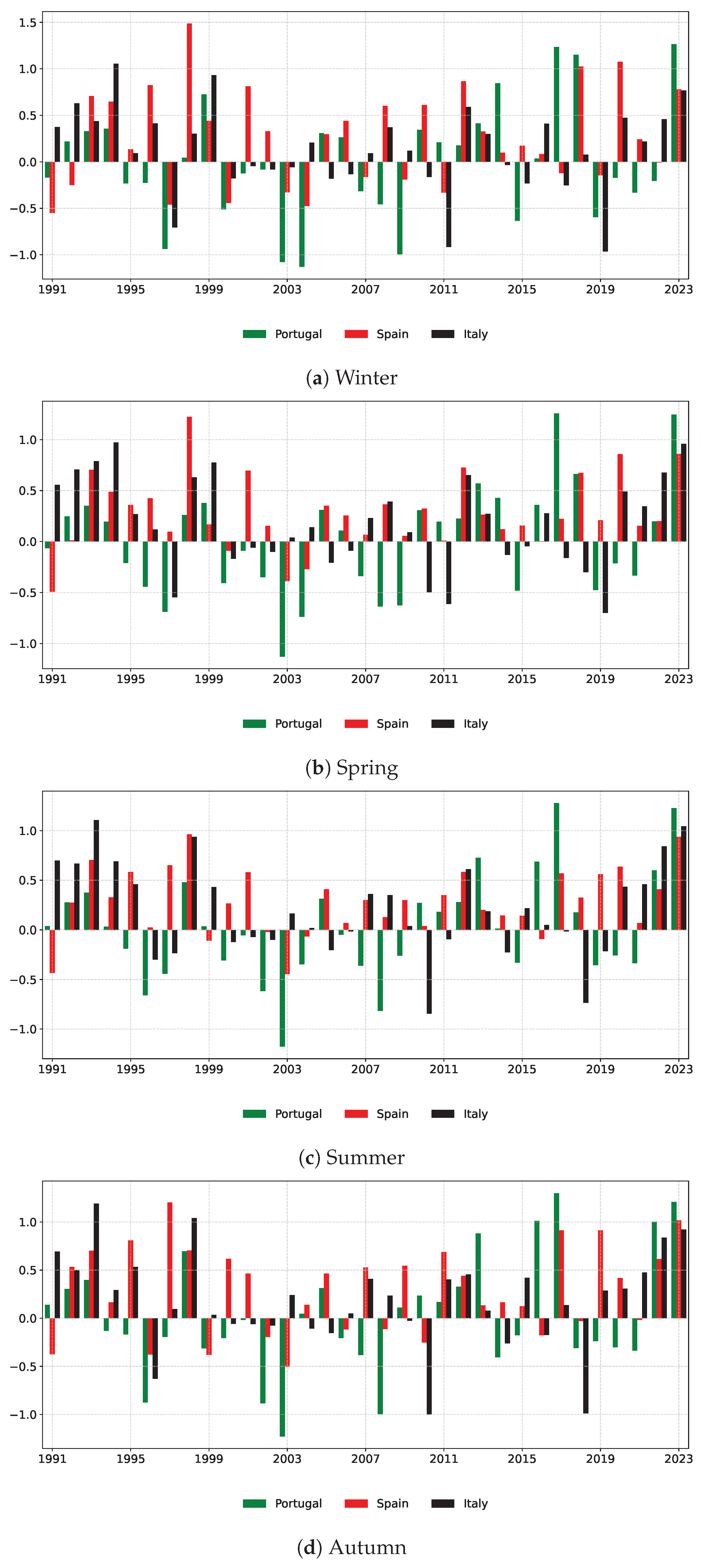
Standardised anomalies for the warm temperature indicator highlight a clear intensification of heat extremes across all seasons in Southern Europe (Figure 15a–d). In winter, Spain and Portugal show an earlier and sharper rise, with values exceeding +2 by the mid-1990s and peaks above +3 in recent years; Portugal reached +5.39 in 2022. Italy follows a delayed but accelerating trajectory, converging towards Iberian values and reaching +3.21 in 2023. In spring, all countries exhibit a consistent upward trend, with only rare reversals. Spain and Portugal record the most extreme anomalies (e.g., 1997, 2015, 2023), while Italy shows a steady rise from the early 2000s, with peaks above +3 in recent years. Over the last decade, anomalies have remained above +1.5 across the Iberian Peninsula, with Italy occasionally surpassing them. Summer shows the sharpest rise in warm anomalies. Italy is the most affected, recording the highest number of extreme years and a peak of +8.29 in 2003. Spain follows with several episodes above +4 and a maximum of +6.48 in 2022, while Portugal shows a more moderate but steady increase. Since 2014, Italy has consistently recorded the highest summer anomalies. In autumn, warming becomes prominent from 2008 onwards. Italy shows the earliest and most persistent anomalies, followed by Spain with a rising trend. Portugal displays mainly positive values in recent years, though rarely exceeding +1. The pattern indicates particularly pronounced autumn warming in the central Mediterranean region.
Figure 16a displays the five-year moving average curves, revealing a sustained rise in standardised warm temperature anomalies across all three countries, albeit with distinct national trajectories. Until the late 1990s, the series show broadly similar patterns, characterised by moderate values and minimal differences between countries. From the early 2000s, however, the Italian curve begins to diverge, rising more sharply and consistently than those of Portugal and Spain and reaching consistently higher values, which indicates a more pronounced and persistent intensification of thermal anomalies. Despite some interannual fluctuations, the Italian series shows a stronger and more continuous warming trajectory. Portugal, while also experiencing a long-term increase, consistently remains below the other two countries.
The French curve (see Figure 2.1, in Garrido et al. 2024, p. 6) remains within a narrow band up to 2003, with values oscillating between +0.7 and just above +1, closely aligning with the Spanish curve. A pronounced increase follows from the mid-2000s, peaking at around +1.6 in 2008, at levels comparable to the Italian curve. This is followed by a temporary decline to +0.7 around 2012, before a renewed and steeper ascent begins. In the final decade of observation, French values position themselves between the Spanish and Portuguese curves, suggesting an intensification of thermal stress across mainland France. Although not reaching the levels observed in Italy or Spain, the recent acceleration indicates convergence towards the warming dynamics seen in Southern Europe.
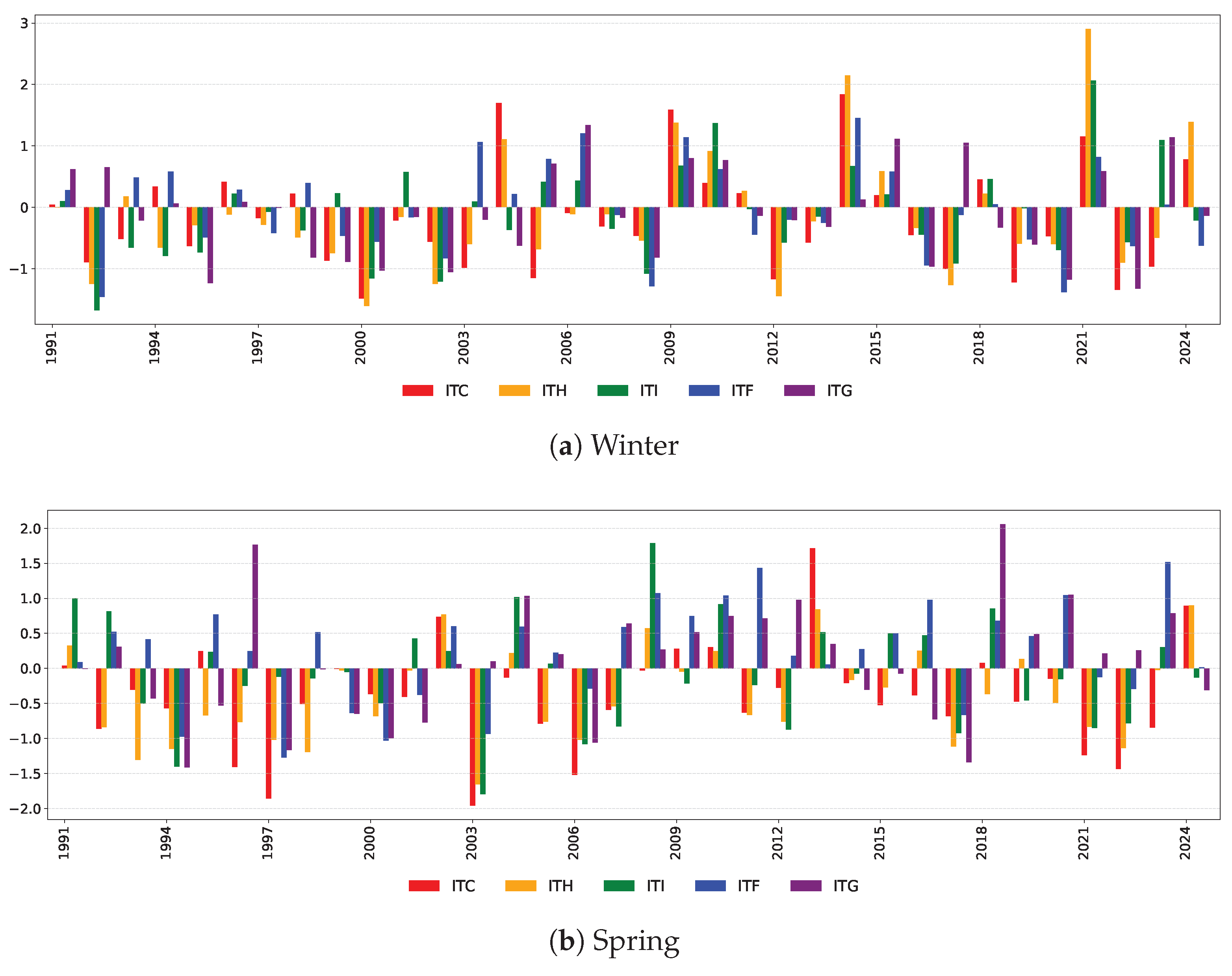
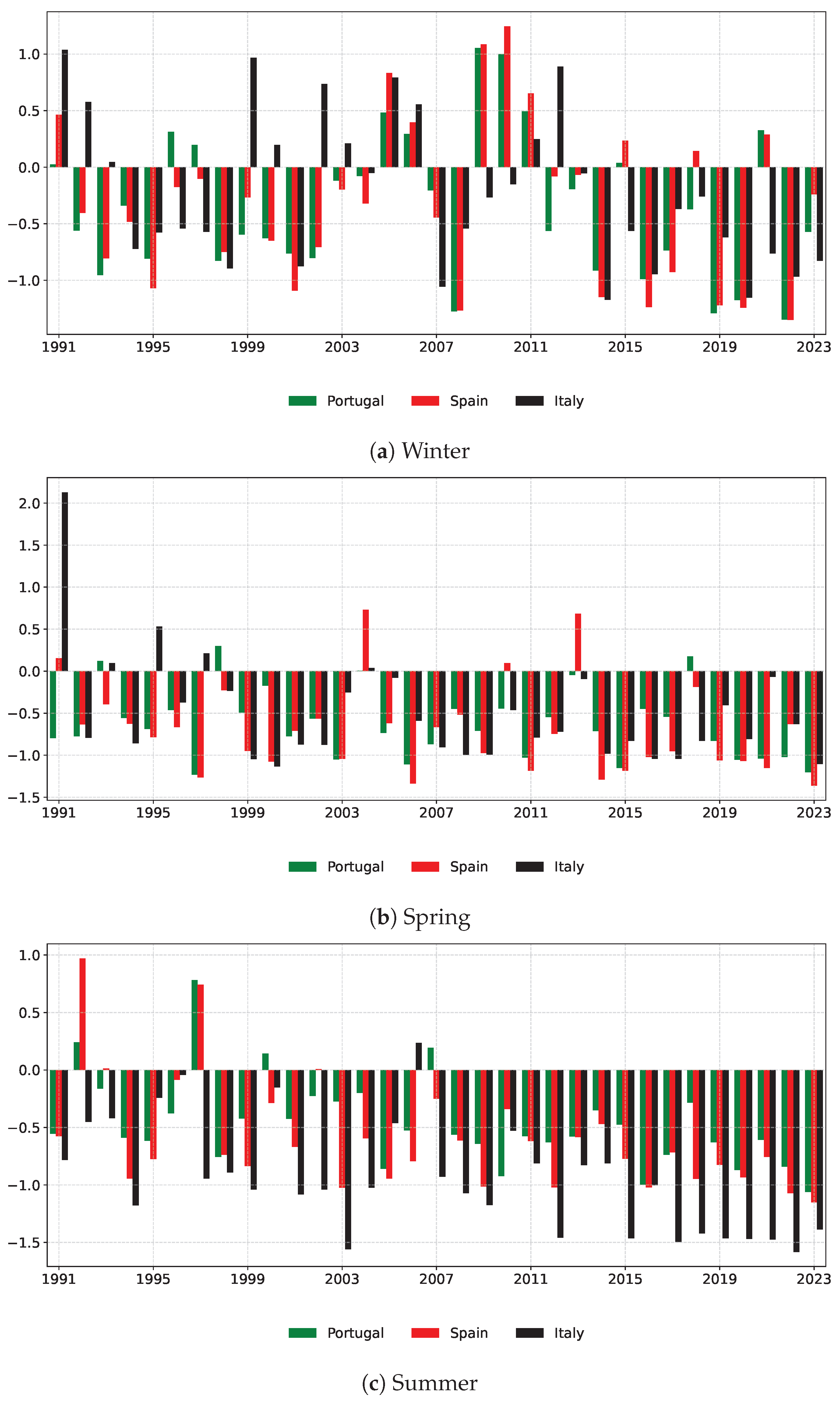
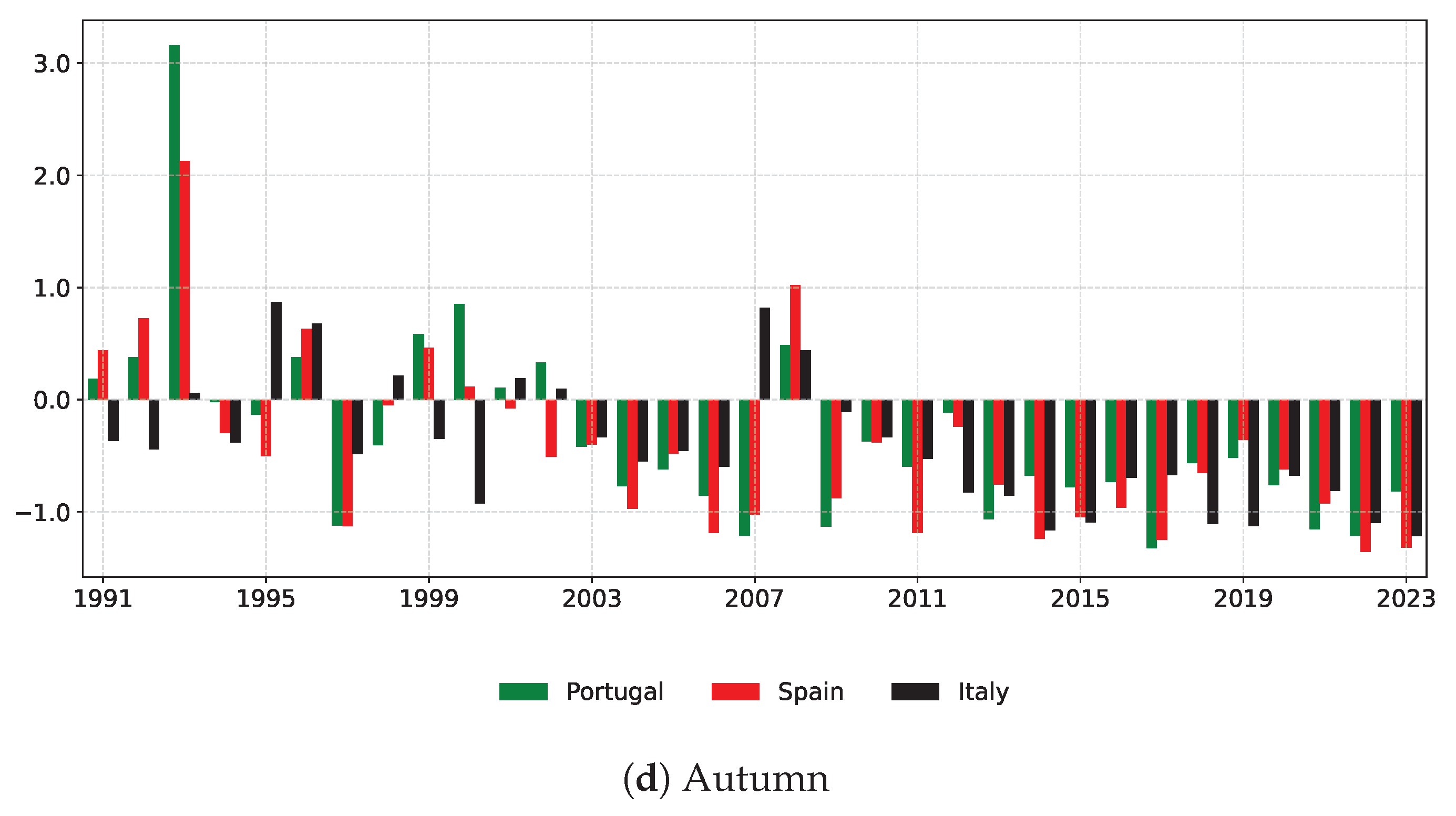
The widespread amplification of heat stress observed across all seasons is mirrored by a corresponding decline in cold extremes, as captured by the Cool Temperature indicator. Standardised anomalies for this indicator reveal a widespread decline in the frequency of cool days and nights across Southern Europe (Figure 17a–d).
In the winter, Spain and Portugal show the earliest and most pronounced reductions (e.g., −1.35 in 2022), while Italy exhibits a delayed but persistent decline from 2014 onwards (e.g., −1.15 in 2020). In spring, the weakening of cold extremes continues, particularly in the Iberian countries, where anomalies frequently fall below −1, indicating a progressive loss of early-season coolness.
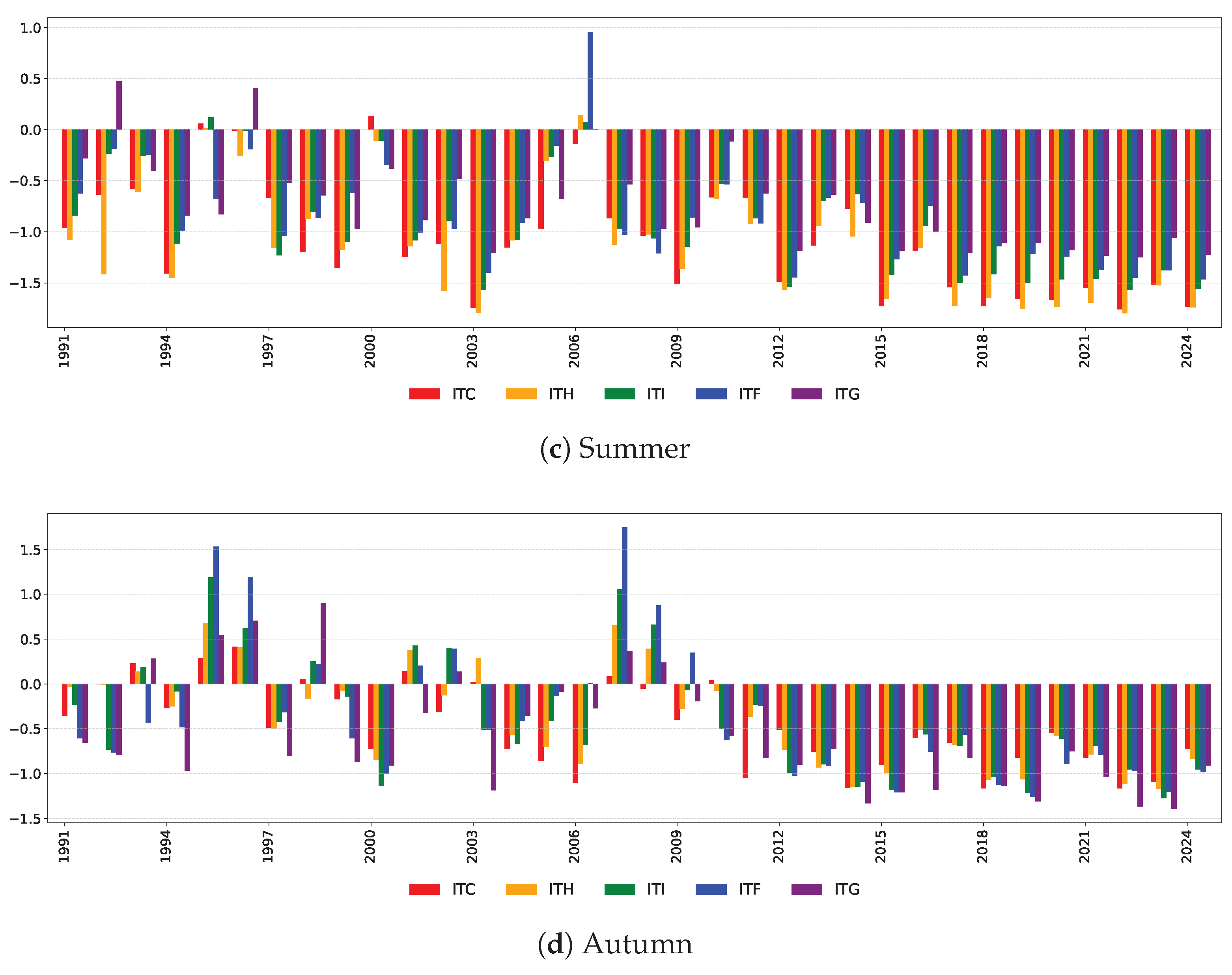
In summer, all three countries exhibit predominantly negative anomalies, reflecting the near disappearance of relatively cool summer conditions. Italy records the most pronounced and consistent decline, with values often approaching −1.5 (e.g., 2003, 2015, 2017, 2022), while Spain stabilises between −0.7 and −1.1 after 2012. Portugal exhibits a milder yet steady downward trend. Autumn confirms this pattern: anomalies have remained consistently below zero since 2009, with notable peaks in recent years for all countries (e.g., −1.36 in 2022 for Spain). No country demonstrates a consistently dominant profile across the autumn series.
To complement the seasonal perspective, the five-year moving averages offer a clearer view of underlying trends by smoothing out short-term variability. As illustrated in Figure 16b, all three countries register a general reduction in the frequency of relatively cool days. Italy follows the sharpest and most consistent downward trajectory, with the largest overall decrease in the moving average series (−0.66), largely driven by the summer season, compared with −0.39 for Spain and −0.34 for Portugal.
When comparing France with the other countries (see Figure 2.1, in Garrido et al. 2024, p. 6), the French trajectory for the Cool Temperature moving average is distinguished by consistently lower values and an earlier onset. The French curve had already reached −1 by the early 2000s and consistently maintained anomalies close to or exceeding −2 for much of the subsequent period. After 2013, it experienced a sharper decline, falling to −1.3 in 2022, a value more negative than those observed in Portugal (−0.75), Spain (−0.80), and Italy (−0.94).
Figure 16c depicts the long-term trend in thermal change, derived from the five-year moving average of net thermal anomalies for the Iberian–Italian cluster. It highlights Italy as the country consistently most exposed to warm extremes, with an upward trajectory mainly driven by summer and autumn.
  • Hydrological Indicators: Precipitation and Drought
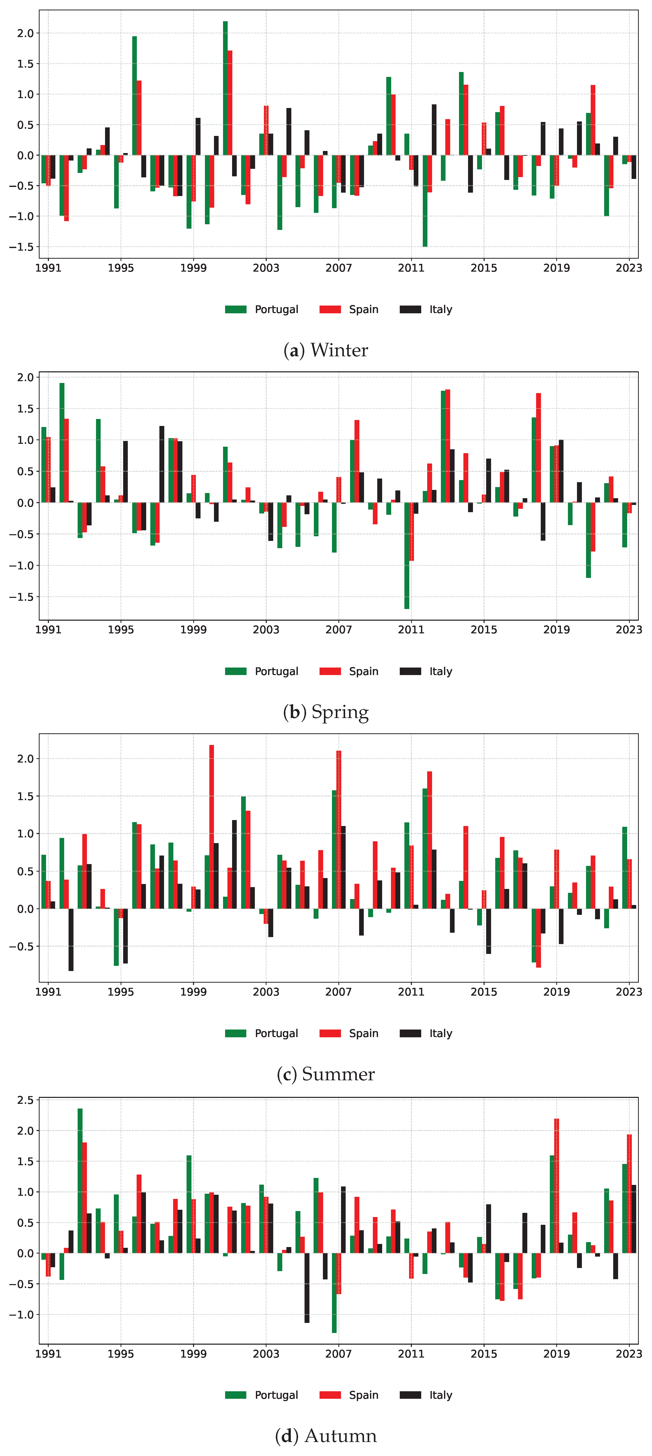
Standardised anomalies of the Precipitation indicator show seasonally differentiated patterns across the three countries (Figure 18a–d). In winter, Portugal exhibits a predominantly negative signal with muted extremes, particularly in 2012 (−1.99), while Spain alternates between wet and dry winters, with marked peaks in 1996 and 2010. Italy deviates from this pattern: after a dry phase up to 2008, a shift towards wetter winters emerges, with strong positive anomalies in 2009, 2014, and a peak of +1.53 in 2021. In spring, negative anomalies prevail before 2000 in all three countries, followed by alternating dry and wet seasons. Portugal and Spain display more pronounced extremes, while Italy’s anomalies remain moderate, mostly within ±1.
Summer anomalies are predominantly negative across the region, indicating a general weakening of extreme rainfall. Spain records the most markedly negative values, with no significant peaks after 1997. Portugal’s rare extremes are confined to the pre-2007 period. Italy differs slightly, with four moderate positive anomalies in recent years, suggesting possible signs of increased convective variability. In autumn, Portugal shows a clear attenuation of extreme events from 2007 onwards, despite persistent instability. Spain maintains moderately positive anomalies with limited variability and a single peak in 2012. Italy registers mostly moderate positive values, with only two seasons (1996 and 2000) exceeding +1, suggesting a regime of above-average but contained autumn precipitation.
These national features are mirrored in the five-year moving averages presented in Figure 19a. In recent years, Portugal has shown the steepest decline, driven by the accumulation of negative seasonal anomalies across all quarters, without compensatory episodes. Spain records a milder decrease, supported by greater seasonal variability. Italy, by contrast, is marked by a sustained positive phase from 2010 to 2018, followed by stabilisation around zero. This pattern reflects the continued absence of persistent negative anomalies, although recent signals suggest more of a halted progression than a fully stable equilibrium.
The five-year moving average curve of the French precipitation indicator (see Figure 2.3, in Garrido et al. 2024, p. 7) shows a mildly oscillating and cyclical pattern. Values fluctuate within a narrow band around zero, typically between −0.1 and +0.1, without any sustained upward or downward trend. In the most recent period, the curve settles slightly above zero, reflecting the recent evolution of the Italian indicator. This behaviour is consistent with recent seasonal averages exceeding +0.3, as reported by Garrido et al. (2024, pp. 6–7), and indicates an increase in variability rather than a structural shift in the long-term signal.
Standardised anomalies for the Drought indicator show diverging seasonal trajectories across Southern Europe (Figure 20a–d). In winter, Spain displays the most persistent signal, with 21 positive anomalies since 1991, indicating longer-than-usual dry spells, 11 of which exceed +0.5. Italy registers frequent but milder anomalies, rarely above +0.5. Portugal presents a more variable pattern: while some intense dry spells occur after 2010, numerous winters (12 since 2001) exhibit negative anomalies, pointing to shortened dry periods and alternating moisture conditions. Italy shows a moderately alternating pattern with both dry and wet winters, lacking a dominant trend.
In spring, Portugal records high interannual variability, with both prolonged dry spells and wetter seasons. Spain maintains a more stable drought signal centred on a consistently elevated mean. Italy diverges, with recent negative anomalies reflecting a partial rebalancing and increased occurrence of shorter dry spells. Summer dynamics confirm structural dryness in Spain, which registers 27 positive anomalies out of 34, including ten above +0.5. Portugal shifts from sustained negative values (1996–2009) to more frequent moderate dry spells after 2010. Italy exhibits the most irregular pattern, alternating phases and recording a new dry peak (+1.04 in 2022). Yet the mean anomaly remains stable over time, suggesting persistent but non-accelerating summer dryness.
In autumn, Spain retains the most consistent dry signal, with 22 positive anomalies and minimal wet seasons since 2011. Portugal moves from an earlier wet regime to renewed dryness after 2010. Italy follows a U-shaped trajectory: early drought, a variable central phase, and recent intensification, with the last five years showing exclusively positive anomalies. This confirms a reactivation of autumn drought conditions in Italy.
The moving averages depicted in Figure 19b summarise drought anomaly trends over time. Spain shows the most persistent positive trajectory. Portugal displays a partial reversal beginning after 2014: the curve gradually rises, turning positive around that year, and is followed by periods of moderate fluctuation, including temporary declines towards zero or slightly negative values, reflecting variability within an overall positive phase. Italy takes a different path: after peaking around 1994, the curve declines until 2006 and then initiates a gradual upward trend, with a marked acceleration after 2019, indicating an emerging long-term drought signal.
France shows a persistently positive long-term drought signal, similar to that of Spain but with generally lower values, indicating a less intense phenomenon (Figure 2.4, in Garrido et al. 2024, p. 7). This stable curve, which remains almost consistently above zero, indicates a subtle increase in the duration of dry spells, without the marked variability observed in Portugal and Italy.
  • Wind Power Indicator
Standardised anomalies for Wind Power show seasonally and geographically differentiated signals across Southern Europe (Figure 21a–d).
In winter, Portugal and Spain register predominantly negative anomalies, with mean values of −0.23 and −0.04 and the highest variability (standard deviations 0.91 and 0.72, respectively). Italy records fewer negative anomalies, a slightly positive mean (+0.02), and the lowest variability (0.43), indicating a more stable winter wind regime.
In spring, extreme wind episodes become more frequent in Portugal and Spain, both of which show numerous positive anomalies despite continued variability, especially in Portugal. Italy displays a milder pattern, with less frequent and lower-intensity anomalies. Mean values are positive in all three countries: Spain (+0.30), Italy (+0.18), and Portugal (+0.11).
Summer wind anomalies intensify over the Iberian Peninsula, with Spain and Portugal recording the highest means (+0.67 and +0.45) and similar variability (0.60). Portugal, however, experiences more frequent negative anomalies, suggesting a less stable signal. Italy diverges again, with a lower mean (+0.17), lower variability (0.50), and more frequent negative anomalies, pointing to fewer and less intense strong wind events.
In autumn, the Iberian countries maintain higher means (+0.39 Portugal, +0.49 Spain) and undergo phases of intense wind activity, including recent peaks. Italy remains comparatively subdued, with a mean of +0.26 and generally moderate anomalies. The Italian pattern increasingly diverges from the Iberian one, often showing opposite anomaly polarities in recent years.
These seasonal patterns shape the trajectories of the five-year moving averages shown in Figure 19c. Spain consistently records the highest values, driven by sustained and intense positive anomalies in spring, summer, and autumn. Portugal and Italy display more moderate trends: the Portuguese curve is influenced by frequent negative anomalies in winter and spring and by pronounced interannual variability. In contrast, the Italian curve, though generally less pronounced, indicates a more stable wind regime and fewer negative values. This results in alternating positions between the two curves over time, with Italy slightly prevailing in recent years owing to its steadier anomaly profile.
The French case shows a general decline in wind power intensity since the early 2000s, suggesting a weakening of extreme wind episodes over the past two decades (Figure 2.5, in Garrido et al. 2024, p. 8). This trend is consistent with those observed in Italy and Portugal, although France records consistently lower values, mostly remaining in the positive range, with the curve staying below 0.2. The five-year moving average has gradually decreased, dipping slightly below zero around 2020 before revealing signs of recovery in the most recent years.
Overall, the comparison of individual indicators confirms the presence of common climate pressures across the European countries considered, together with national specificities that require monitoring at the country level. Developed in line with the IACI and FACI frameworks, ITACI provides a consistent interpretation of climate anomalies in Italy, while also enhancing European comparability.

6.3. Sea Level Dynamics in a Comparative Perspective: The Italian Specificities

The Sea Level component shows the strongest correlation with the national ITACI (Figure 12), a feature also observed in the Iberian and French indices. Further evidence comes from Cheung et al. (2024), who report a significant long-term link between sea level variations and crop yields, reinforcing the potential role of sea level as a relevant factor in insurance modelling. This justifies dedicating a specific analysis to sea level dynamics within the Italian context.
The five-year moving average of the Sea Level indicator for Italy displays a distinct pattern compared with those of the Iberian Peninsula and France (see Figure 22 and Figure 2.6, in Garrido et al. 2024, p. 8). Both the Iberian Peninsula and France experienced an upward acceleration in sea level anomalies starting in the mid-1990s. While the Iberian curve continues to rise steadily, exceeding +4 in recent years, the French curve shows signs of deceleration over the past decade, entering a plateau phase. In contrast, the Italian curve exhibits a quasi-decadal oscillatory pattern, with alternating phases of positive and negative anomalies generally ranging within ±1. Since 2011, however, values have remained consistently positive, marking a recent phase of moderate growth.
The distinct behaviour observed in the Italian curve reflects the unique characteristics of the Mediterranean Sea, a semi-enclosed basin governed by specific dynamics that differ substantially from those of the open ocean. Several studies have reported that the sea level in the Mediterranean has increased, but at a slower rate than the global and European mean (see, for instance, Tsimplis and Baker 2000; Vigo et al. 2011; Zerbini et al. 2017; Melet et al. 2024).
A first key difference lies in the underlying mechanisms that drive sea level changes. At the global scale, sea level rise is primarily driven by two components: the mass contribution from the melting of continental ice sheets, which accounts for around 80% of the observed rise, and the steric component, referring to the expansion of seawater volume caused by rising temperatures (thermal expansion), responsible for about 20% (Fox-Kemper et al. 2021; Milne et al. 2009). In contrast, in the Mediterranean Sea, the steric contribution plays only a minor role, as thermal expansion is largely offset by salinity-induced contraction. Moreover, the Mediterranean sea level is characterised by pronounced regional variability, resulting from its unique morphology, salinity gradients, high evaporation rates, and complex internal circulation patterns. In particular, the basin has an irregular shape, with multiple sub-basins (e.g., Adriatic, Ionian, Aegean), narrow straits, and variable bathymetry. This configuration strongly influences circulation dynamics, causing different water masses to move in a complex and localised manner. Specifically, the anti-estuarine circulation regime, in which dense, saline waters flow outward towards the ocean while lighter, less saline waters enter at the surface, and buoyancy forcing, referring to density changes driven by variations in temperature and salinity, play a crucial role in shaping these regional features.
Recent studies have further shown that sea level changes in the Mediterranean are primarily influenced by mass-related processes such as evaporation, precipitation, river runoff, and exchanges through straits (Borile et al. 2025). Accordingly, the dominant driver is the water budget, defined as the net balance of all inflows and outflows, including evaporation, precipitation, runoff, and oceanic exchange. As a result, regional dynamics and the water budget exert a stronger influence than temperature in determining sea level changes in the Mediterranean.
The Mediterranean sea level trend is neither temporally nor spatially uniform: the Western Mediterranean shows an accelerating trend, whereas the Eastern Mediterranean is experiencing a deceleration. Borile et al. (2025) report that, over the past three decades, there has been a reversal in sea level trends between the western and eastern Mediterranean, with recent decadal trends highlighting an acceleration in the western basin and a slowdown in the eastern basin. Specifically, in recent decades, the Eastern Mediterranean has experienced reduced water input due to increased evaporation and decreased precipitation, runoff, and freshwater inflow.
The Adriatic Sea displays distinct local dynamics strongly influenced by regional factors (e.g., salinity, evaporation, internal circulation) and makes a significant contribution to the observed slowdown in Mediterranean sea level rise. Early results, based on both historical records and future projections, suggest that sea level in the Adriatic is not rising steadily but instead shows signs of deceleration and, under certain conditions, could even decline (Borile et al. 2025). This pattern extends to other Mediterranean sub-basins, reflecting similar regional mechanisms of sea level variability.
These regional dynamics help explain the observed differences when comparing standardised anomaly figures for Italy with those for the Iberian Peninsula and France, which are more directly influenced by oceanographic components.
Looking at Figure 23, alternating periods of positive and negative standardised anomalies can be observed, with shifts occurring at roughly quasi-decadal intervals. Three distinct negative phases begin in the early 1970s, around 1987, and around 2001.
This quasi-decadal pattern is likely linked to circulation reversal episodes associated with the North Ionian Gyre (NIG), which drives alternating cyclonic and anticyclonic phases. These phases correspond to a rising (falling) sea level trend in the Ionian Sea, accompanied by a falling (rising) trend in other Mediterranean sub-basins during cyclonic (anticyclonic) conditions, a phenomenon referred to as the “breathing oscillation” (see Meli and Romagnoli 2022; Meli 2024). This pattern appears to propagate across Mediterranean sub-basins, with a more pronounced effect east of the Sicily Channel, while its impact in the western basin remains unclear and difficult to interpret. The pronounced negative values in the late 1980s and early 1990s, particularly in winter and spring, may be associated with an intense oceanographic event: the Eastern Mediterranean Transient (EMT). These fluctuations are less evident in the earlier part of the time series, as this period defines the baseline for anomaly calculation.
The quasi-decadal signal emerges more clearly in winter and spring, when alternating positive and negative phases are more distinct and appear aligned with circulation reversals. However, the negative phase observed in the early 2000s also affected summer and autumn, albeit with lower intensity. This further supports the quasi-decadal nature of the signal, characterised by alternating phases across the entire Mediterranean basin. In recent years, summer and autumn have exhibited a strong and persistent positive trend, particularly during the warm season, contributing to an upward tendency in the five-year moving average. This seasonal contrast is also evident in the mean (non-standardised) anomalies, which show negative values in winter and spring and increasingly positive values in summer and autumn, with the latter displaying the highest deviations (see Figure 24). These findings suggest a progressive strengthening of the sea level signal during the warmer and transitional seasons.
Overall, the strong correlation between the national ITACI and Sea Level, the highest among all components, underscores the importance of marine factors in Italy’s climate risk assessment. Although Mediterranean sea level dynamics display distinct temporal patterns compared with neighbouring European regions, the strength of the ITACI–Sea Level relationship is consistent with the high correlations observed elsewhere in Europe.

7. Conclusions

This paper presents the development of ITACI and its application to the spatial and temporal assessment of climate risk across Italy, with the aim of supporting climate-informed decision-making and insurance design. ITACI builds on the methodological framework of the ACI, previously adapted for France (FACI) and the Iberian Peninsula (IACI). It draws on high-resolution ERA5-Land data together with long-term sea level records to capture multiple dimensions of climate anomalies. By combining scientific rigour with practical applicability, ITACI provides a foundation for a more resilient and data-driven approach to climate risk management in Italy.
This study shows that Italy’s complex climatic variability, extensive coastline, low insurance penetration and persistent protection gaps make the development of a technically sound and locally calibrated index for climate risk assessment particularly urgent (see Section 2). ITACI addresses this need by providing a high-resolution multi-hazard framework aligned with Italy’s specific exposure profile. It offers a scientifically rigorous basis for enhancing risk awareness and designing innovative insurance mechanisms in response to increasing climate-related losses and recent regulatory initiatives.
Within a broader European context, ITACI complements existing national indices such as FACI (France) and IACI (Iberian Peninsula). Together, these indices contribute to a harmonised European framework for climate diagnostics and policy coordination, laying the foundation for coherent risk assessment approaches consistent with the EU’s climate resilience objectives. The comparative analysis highlights the specificity of Italy’s exposure profile. Although all three countries show a clear warming signal and increasing climate anomalies, our results indicate that Italy follows a more fragmented and distinctive trajectory. Since the 1990s, the Italian curve has remained systematically below its French and Iberian counterparts, with a unique dip between 2002 and 2008 that is absent elsewhere, before entering a sustained upward phase culminating in 2023.
At the level of individual components, further divergences become apparent. Warm temperature anomalies in Italy reach higher peaks than in Iberia and remain more persistent thereafter. Italy also displays the earliest and most consistent positive autumn anomalies, indicating a Mediterranean-specific warming pattern. By contrast, cool temperature anomalies show the steepest and most continuous decline in Europe, particularly in summer, albeit with a temporal lag compared with France. Hydrological indicators provide additional contrasts: Italy has recorded wetter winters and occasional positive summer rainfall anomalies, diverging from the persistently dry Iberian signals, while autumn precipitation remains moderately positive compared with Portugal’s marked post-2007 decline. Drought follows a U-shaped trajectory, whereas Spain shows a consistently strong profile and France a milder one. For wind power, Italy exhibits a more stable and less extreme pattern, often of opposite sign to Iberian values.
The sea level component represents one of the most innovative aspects of our findings, reflecting the specific dynamics of the Mediterranean basin, which differ substantially from those observed in countries with both Atlantic and Mediterranean coasts. Unlike the steady rise recorded in the Iberian Peninsula or the plateau phase in France, Italy displays quasi-decadal oscillations linked to Mediterranean-specific processes such as the North Ionian Gyre reversals and the Eastern Mediterranean Transient. These oscillations, by introducing temporary reversals, directly influence the trajectory of ITACI and add a distinctive marine-driven variability to the index.
A key finding is that analyses at the macroarea scale reveal signals that would otherwise be obscured in national aggregation, reinforcing the importance of regionally disaggregated indices. In particular, we observe early signals in the North-West, pronounced hydrological variability in the North-East, structural drought in Central Italy, a recent acceleration in the South and chronic dryness in the Islands. These results confirm the heterogeneity of Italian climate stress and suggest that a single national parametric policy could be ineffective or entail substantial basis risk, pointing instead to the need for regionally calibrated indices. Similarly, a uniform national adaptation strategy may fail to capture critical local specificities, indicating that climate adaptation measures should be geographically tailored.
Recent empirical evidence from Spain shows that ACI-type indices can serve as effective triggers for index-based agricultural insurance, suggesting that ITACI could provide a robust foundation for similar applications in Italy. The growing institutional interest in parametric insurance, exemplified by its inclusion among eligible subsidised instruments for the agricultural sector in Italy’s 2024 Risk Management Plan (PGRA), highlights the increasing policy attention devoted to such tools. This context suggests that scientifically robust indices such as ITACI have the potential to support national risk mitigation strategies. Further research could explore ITACI’s applicability to other climate-sensitive sectors, such as renewable energy production, water resource management and infrastructure planning, where exposure to climate variability is becoming increasingly critical. ITACI could also be integrated into catastrophe-linked securities or regulatory stress-testing frameworks, thereby strengthening climate resilience planning and supporting more robust financial risk management strategies.
This study offers important implications and outlines directions for future research. From an actuarial perspective, the ITACI framework can provide objective, transparent and regularly updated indicators that may substantially support the calibration of index-based insurance products. Moreover, ITACI can serve as a key tool to inform public policy and guide climate adaptation strategies at both national and regional levels, enabling consistent monitoring of evolving climate risks and the development of pre-disaster interventions.
Although the current indicators are aligned with internationally recognised standards (IPCC 2013), further improvements could be achieved by integrating additional metrics capable of capturing critical climate dimensions such as drought persistence, compound events and short-lived extremes, thereby broadening the relevance and robustness of the index. In this regard, the set of indices developed by the Expert Team on Climate Change Detection and Indices (Expert Team on Climate Change Detection and Indices 2023), widely used to monitor thermal, hydrological and drought extremes, provides a useful reference for potential future extensions.
In addition, the adoption of such alternative metrics would not only refine the representation of climate dynamics but also foster the development of thematic or sector-specific versions of the index. The selective inclusion of indicators such as SPI or soil moisture anomalies would enable the capture of specific dimensions of climate risk and support targeted applications, including agricultural resilience, infrastructure vulnerability and compound hazard monitoring.
Even if the ITACI is defined here as a historical index, its framework could in principle be combined with climate simulation models (e.g., CMIP6) to generate future projections of its components. Exploring such predictive applications lies beyond the scope of this paper.
Finally, future developments could extend the application of ITACI beyond agriculture and coastal risk, exploring its use in pricing catastrophe-linked securities, informing reinsurance strategies and supporting solvency assessments under climate-related stress scenarios.
Consequently, ITACI may become a cornerstone of national climate risk strategies in Italy, while also contributing to broader European coordination, enabling data-driven decision-making, fostering resilience and supporting coherent policy development in the face of escalating climate challenges.

Author Contributions

Conceptualization, J.G.; Methodology, J.G.; Software, B.R.; Investigation, B.R. and S.D.; Validation, B.R. and S.D.; Data curation, B.R. and S.D.; Visualization, B.R.; Writing—original draft preparation, B.R.; Writing—review and editing, B.R. and J.G.; Supervision, J.G. All authors have read and agreed to the published version of the manuscript.

Funding

Garrido gratefully acknowledges the financial support of the Chaire d’Excellence Digital Insurance And Long term risk—DIALog; for details, see https://chaire-dialog.fr/ (accessed on 27 September 2025).

Data Availability Statement

The raw data supporting the conclusions of this article will be made available by the authors on request.

Acknowledgments

The authors wish to thank Matteo Meli (Department of Biological, Geological and Environmental Sciences, University of Bologna) for his valuable support in the selection and analysis of sea level data. His expertise in sea level variability has been instrumental in refining the treatment of this component within the ITACI framework. The authors would also like to thank the anonymous reviewers for their constructive comments, which have contributed to improving the clarity and robustness of this manuscript.

Conflicts of Interest

The authors declare no conflict of interest.

Appendix A. Spatial Distribution of the Seasonal ITACI from 2012 to 2022
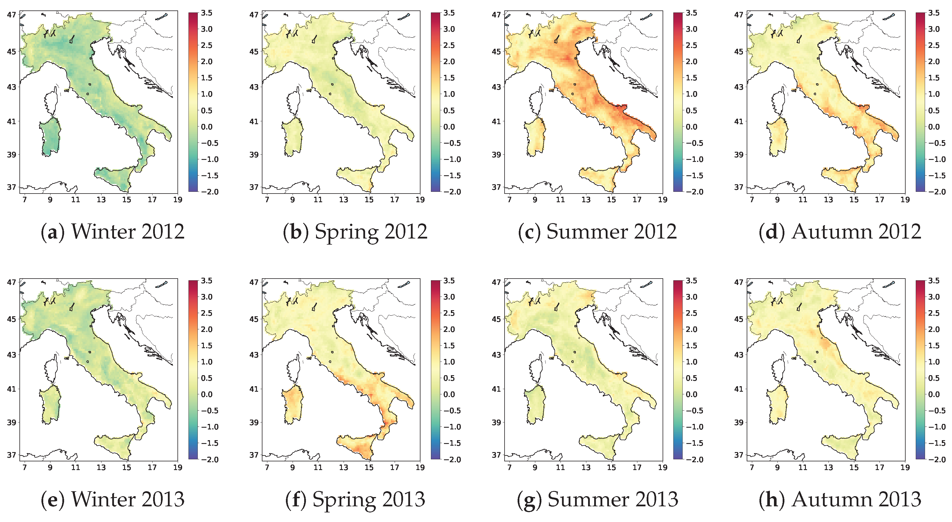
Figure A1. Spatial distribution of ITACI by season at 0.1° × 0.1° resolution from 2012 to 2017.
Risks 13 00192 g0a1aRisks 13 00192 g0a1b
Figure A2. Spatial distribution of ITACI by season at 0.1° × 0.1° resolution from 2018 to 2022.
Risks 13 00192 g0a2aRisks 13 00192 g0a2b

Appendix B. Standardised Anomalies Across Macroareas by Climate Indicator
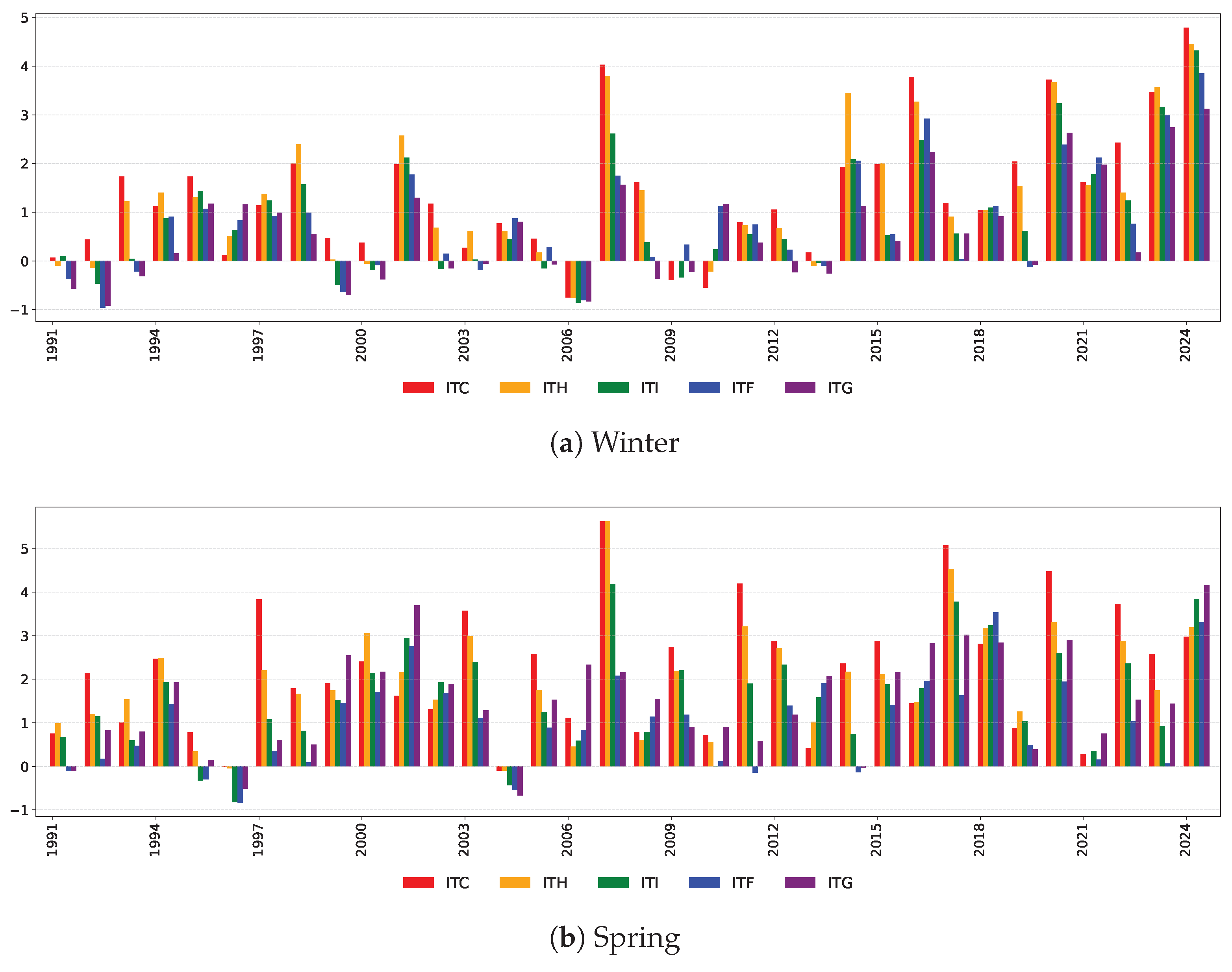
Figure A3. Standardised anomalies of Warm Temperature component by season for NUTS1 macro-areas from 1991 to 2024. NUTS1 codes are as follows: North-West (ITC), North-East (ITH), Centre (ITI), South (ITF), and Islands (ITG).
Risks 13 00192 g0a3aRisks 13 00192 g0a3b
Figure A4. Standardised anomalies of Cool Temperature component by season for NUTS1 macro-areas from 1991 to 2024. NUTS1 codes are as follows: North-West (ITC), North-East (ITH), Centre (ITI), South (ITF), and Islands (ITG).
Risks 13 00192 g0a4aRisks 13 00192 g0a4b
Figure A5. Standardised anomalies of Precipitation component by season for NUTS1 macro-area from 1991 to 2024. NUTS1 codes are as follows: North-West (ITC), North-East (ITH), Centre (ITI), South (ITF), and Islands (ITG).
Risks 13 00192 g0a5aRisks 13 00192 g0a5b
Figure A6. Standardised anomalies of Drought component by season for NUTS1 macro-areas from 1991 to 2024. NUTS1 codes are as follows: North-West (ITC), North-East (ITH), Centre (ITI), South (ITF), and Islands (ITG).
Risks 13 00192 g0a6aRisks 13 00192 g0a6b
Figure A7. Standardised anomalies of Wind Power component by season for NUTS1 macro-areas from 1991 to 2024. NUTS1 codes are as follows: North-West (ITC), North-East (ITH), Centre (ITI), South (ITF), and Islands (ITG).
Risks 13 00192 g0a7aRisks 13 00192 g0a7b

Notes

1
As defined by EIOPA (2019), “Physical risks from climate change arise from a number of factors, and relate to specific weather events (such as heatwaves, floods, wildfires, and storms) and longer-term shifts in the climate (such as changes in precipitation, extreme weather variability, sea level rise, and rising mean temperatures). Some examples of physical risks crystallising include the following: increased frequency, severity, or volatility of extreme weather events impacting property and casualty insurance and increased frequency and severity of flooding leading to physical damage to the value of financial assets or collateral held by banks, such as household and commercial property.” See also EIOPA (2022), which provides consistent definitions and examples.
2
Data extracted from the Excel file provided by EIOPA as part of the 2024 Insurance Protection Gap Dashboard, available at: https://www.eiopa.europa.eu/tools-and-data/dashboard-insurance-protection-gap-natural-catastrophes_en (accessed on 16 April 2025).
3
A seminar on the topic was organised by IVASS, entitled “Parametric insurance: between market, technology and law”, and held on 10 May 2024.
4
Air quality indicators are not included in the ITACI framework in order to ensure full comparability with the other indices in the ACI family (ACI, FACI, IACI), which are exclusively based on climate-driven variables. While air quality is highly relevant for environmental and health studies, it falls outside the scope of this climate-focused index and may be considered in future extensions.
5
Consistently, December refers to the previous year l 1 .
6
Since anomalies are expressed in different units, magnitude comparisons are meaningful only within the same indicator across seasons.
7
The numerical time series of the IACI for Portugal and Spain is publicly available at https://e-actuaries.eu/downloads/iberian-actuarial-climate-index/ (accessed on 16 April 2025), whereas the FACI series for France has not been released.

References

  1. Aiello, Maria A., Cristina Angelico, Piero Cova, and Valentina Michelangeli. 2024. Climate-related Risks for Italy: An Analysis Based on the Latest NGFS Scenarios. Banca d’Italia, Occasional Papers 847. Available online: https://www.bancaditalia.it/pubblicazioni/qef/2024-0847/QEF_847_24.pdf?language_id=1 (accessed on 26 April 2024).
  2. ANIA. 2024. L’Assicurazione Italiana 2023–2024. Available online: https://www.ania.it/documents/35135/439653/LAssicurazione-Italiana-2024_WEB.pdf/bf8d4d10-b3ce-45d0-62c7-76d57492be13?t=1719994663305 (accessed on 15 June 2025).
  3. Aon. 2024. 2024 Weather, Climate and Catastrophe Insight. Available online: https://assets.aon.com/-/media/files/aon/reports/2024/climate-and-catastrophe-insights-report.pdf (accessed on 15 July 2025).
  4. Borile, Federica, Nadia Pinardi, Vladyslav Lyubartse, Mahmud H. Ghani, Antonio Navarra, Jacopo Alessandri, Emanuela Clementi, Giovanni Coppini, Lorenzo Mentaschi, Giorgia Verri, and et al. 2025. The Eastern Mediterranean Sea Mean Sea Level Decadal Slowdown: The Effects of the Water Budget. Frontiers in Climate 7: 1472731. Available online: https://www.frontiersin.org/articles/10.3389/fclim.2025.1472731/full (accessed on 24 March 2024). [CrossRef]
  5. Casualty Actuarial Society. 2024. Virtual Climate Risk Seminar, Session 4: Actuaries Climate Index 2.0: Improving Geographic Coverage and Extremes Tracking. Available online: https://www.casact.org/event/2024-cas-virtual-climate-risk-seminar (accessed on 3 September 2025).
  6. Cheung, Eric C. K., Ryan H. L. Ip, Ho On Tam, and Jae-Kyung Woo. 2024. Cointegration Analysis of Crop Yields and Extreme Weather Factors Using Actuaries Climate Index with Application of Bonus–Malus System. North American Actuarial Journal, 1–19. [Google Scholar] [CrossRef]
  7. Copernicus Climate Change Service (C3S). 2025. ERA5-Land Hourly Data from 1950 to Present. Available online: https://cds.climate.copernicus.eu/datasets/reanalysis-era5-land?tab=download (accessed on 10 October 2024).
  8. Curry, Charles L. 2015. Extension of the Actuaries Climate Index to the UK and Europe: A Feasibility Study. Institute and Faculty of Actuaries. Available online: https://www.actuaries.org.uk/system/files/field/document/UK_ACI_scoping_FINAL.pdf (accessed on 1 September 2023).
  9. De Vivo, Carmela, Giuliana Barbato, Marta Ellena, Vincenzo Capozzi, Giorgio Budillon, and Paola Mercogliano. 2023. Climate-Risk Assessment Framework for Airports under Extreme Precipitation Events: Application to Selected Italian Case Studies. Sustainability 15: 7300. [Google Scholar] [CrossRef]
  10. EIOPA. 2019. Application Guidance on ORSA. Available online: https://www.eiopa.europa.eu/document/download/d5ae4db7-cc30-40db-ad5e-045876e3c7b3_en?filename=Opinion%20on%20Sustainability%20within%20Solvency%20II%20%28EIOPA-BoS-19/241%29%E2%80%8B.pdf (accessed on 10 June 2025).
  11. EIOPA. 2022. Application Guidance on Running Climate Change Materiality Assessment and Using Climate Change Scenarios in the ORSA. Available online: https://www.eiopa.europa.eu/document/download/5a671bdb-aef7-4c4f-ae31-00c70e640d27_en?filename=Application%20guidance%20on%20running%20climate%20change%20materiality%20assessment%20and%20using%20climate%20change%20scenarios%20in%20ORSA.pdf (accessed on 10 June 2025).
  12. EIOPA. 2024. The Dashboard on Insurance Protection Gap for Natural Catastrophes in a Nutshell. Available online: https://www.eiopa.europa.eu/tools-and-data/dashboard-insurance-protection-gap-natural-catastrophes_en (accessed on 15 May 2025).
  13. European Commission. 2015. Commission Delegated Regulation (EU) 2015/35 of 10 October 2014 Supplementing Directive 2009/138/EC of the European Parliament and of the Council on the Taking-Up and Pursuit of the Business of Insurance and Reinsurance (Solvency II). Official Journal of the European Union L 12: 1–797. Available online: https://eur-lex.europa.eu/legal-content/EN/TXT/?uri=CELEX:32015R0035 (accessed on 20 January 2025).
  14. European Commission. 2021. Commission Delegated Regulation (EU) 2021/1256 of 21 April 2021 Amending Delegated Regulation (EU) 2015/35 as Regards the Integration of Sustainability Risks in the Governance of Insurance and Reinsurance Undertakings. Official Journal of the European Union L 277: 14–16. Available online: https://eur-lex.europa.eu/legal-content/EN/TXT/?uri=CELEX:32021R1256 (accessed on 20 January 2025).
  15. European Parliament and Council. 2003. Regulation (EC) No 1059/2003 of 26 May 2003 on the Establishment of a Common Classification of Territorial Units for Statistics (NUTS). Consolidated version of 1 January 2024. Official Journal of the European Union L 154: 1–41. Available online: https://eur-lex.europa.eu/legal-content/EN/TXT/?uri=CELEX:02003R1059-20240101 (accessed on 20 August 2025).
  16. Expert Team on Climate Change Detection and Indices. 2023. List of Climate Change Indices. Available online: https://etccdi.pacificclimate.org/list_27_indices.shtml (accessed on 10 May 2025).
  17. Figueiredo, Rui, Mario L. V. Martina, David B. Stephenson, and Benjamin D. Youngman. 2018. A Probabilistic Paradigm for the Parametric Insurance of Natural Hazards. Risk Analysis 38: 2400–14. [Google Scholar] [CrossRef]
  18. Fox-Kemper, Baylor, Helen T. Hewitt, Cunde Xiao, Guðfinna Aðalgeirsdóttir, Sybren S. Drijfhout, Tamsin L. Edwards, Nicholas R. Golledge, Mark Hemer, Robert E. Kopp, Gerhard Krinner, and et al. 2021. Ocean, Cryosphere and Sea Level Change. In Climate Change 2021: The Physical Science Basis. Contribution of Working Group I to the Sixth Assessment Report of the Intergovernmental Panel on Climate Change. Edited by Valérie Masson-Delmotte, Panmao Zhai, Anna Pirani, Sarah L. Connors, Clotilde Péan, Sophie Berger, Nada Caud, Yang Chen, Leah Goldfarb, Melissa I. Gomis and et al. Cambridge and New York: Cambridge University Press, pp. 1211–362. [Google Scholar] [CrossRef]
  19. Gao, Lisa, and Peng Shi. 2025. Risk modeling of property insurance claims from weather events. ASTIN Bulletin: The Journal of the IAA 55: 242–62. [Google Scholar] [CrossRef]
  20. Garrido, José, Xavier Milhaud, and Anani Olympio. 2024. The Definition of a French Actuarial Climate Index; One More Step Towards a European Index. Preprint. Available online: https://www.researchgate.net/publication/376982040 (accessed on 15 March 2024).
  21. Hernández-Rojas, Luis F., Adriana L. Abrego-Perez, Fernando E. Lozano Martínez, Carlos F. Valencia-Arboleda, Maria C. Diaz-Jimenez, Natalia Pacheco-Carvajal, and Juan J. García-Cárdenas. 2023. The Role of Data-Driven Methodologies in Weather Index Insurance. Applied Sciences 13: 4785. [Google Scholar] [CrossRef]
  22. IPCC. 2013. Climate Change 2013: The Physical Science Basis. Contribution of Working Group I to the Fifth Assessment Report of the Intergovernmental Panel on Climate Change. Edited by Thomas F. Stocker, Dahe Qin, Gian-Kasper Plattner, Melinda M. B. Tignor, Simon K. Allen, Judith Boschung, Alexander Nauels, Yu Xia, Vincent Bex and Pauline M. Midgley. Cambridge and New York: Cambridge University Press, p. 1535. Available online: https://www.ipcc.ch/report/ar5/wg1/ (accessed on 20 August 2025).
  23. ISTAT. 2022. Attività Antropiche e Salute delle Coste. Indicatori Territoriali di Rischio e Sostenibilità per Aree Costiere e Insulari in Italia e nell’Unione Europea. Available online: https://www.istat.it/wp-content/uploads/2022/09/Attivit%C3%A0-antropiche-e-salute-delle-coste_Ebook.pdf (accessed on 10 May 2025).
  24. IVASS. 2021. Regulation No. 38 of 3 July 2018, on the System of Governance Pursuant to Articles 30, 31 and 32 of Legislative Decree No. 209 of 7 September 2005 – Private Insurance Code, as Amended by the Measure of 9 June 2021. Available online: https://www.ivass.it/normativa/nazionale/secondaria-ivass/regolamenti/2018/n38/index.html?com.dotmarketing.htmlpage.language=1 (accessed on 15 March 2025).
  25. IVASS. 2025. Audizione del Prof. Riccardo Cesari Consigliere dell’Istituto per la Vigilanza sulle Assicurazioni—IVASS. Commissione VIII (Ambiente, Territorio e Lavori Pubblici) della Camera dei Deputati. Available online: https://www.ivass.it/media/interviste/intervista/rc-9-4-25-catastrofali/?dotcache=refresh (accessed on 15 April 2025).
  26. Lin, Xiao, and W. Jean Kwon. 2020. Application of Parametric Insurance in Principle-Compliant and Innovative Ways. Risk Management and Insurance Review 23: 121–50. [Google Scholar] [CrossRef]
  27. Liu, Zhonglu, Shuguang He, Wenjiao Men, and Haibo Sun. 2024. Impact of Climate Risk on Financial Stability: Cross-Country Evidence. International Review of Financial Analysis 92: 103096. [Google Scholar] [CrossRef]
  28. Lomelí-Quintero, Victor-Manuel, Felicitas Calderón-Vega, Cesar Mösso, Agustin Sánchez-Arcilla, and Adrian-David García-Soto. 2023. Impact Costs Due to Climate Change along the Coasts of Catalonia. Marine Science and Engineering 11: 1939. [Google Scholar] [CrossRef]
  29. Melet, Angélique, Roderik de Wal, Angel Amores, Arne Arns, Alisée A. Chaigneau, Irina Dinu, Ivan D. Haigh, Tim H. J. Hermans, Piero Lionello, Marta Marcos, and et al. 2024. Sea Level Rise in Europe: Observations and Projections. In Sea Level Rise in Europe: 1st Assessment Report of the Knowledge Hub on Sea Level Rise (SLRE1). Edited by Bart van den Hurk, Nadia Pinardi, Thorsten Kiefer, Kate Larkin, Petra Manderscheid and Kristin Richter. Göttingen: Copernicus Publications, vol. 3, chap. 4. [Google Scholar] [CrossRef]
  30. Meli, Matteo. 2024. The Potential Recording of North Ionian Gyre’s Reversals as a Decadal Signal in Sea Level During the Instrumental Period. Scientific Reports 14: 4907. [Google Scholar] [CrossRef] [PubMed]
  31. Meli, Matteo, and Claudia Romagnoli. 2022. Evidence and Implications of Hydrological and Climatic Change in the Reno and Lamone River Basins and Related Coastal Areas (Emilia-Romagna, Northern Italy) over the Last Century. Water 14: 2650. [Google Scholar] [CrossRef]
  32. Mills, Evan. 2005. Insurance in a Climate of Change. Science 309: 1040–44. [Google Scholar] [CrossRef]
  33. Milne, Glenn A., W. Roland Gehrels, Chris W. Hughes, and Mark E. Tamisiea. 2009. Identifying the Causes of Sea-Level Change. Nature Geoscience 2: 471–78. [Google Scholar] [CrossRef]
  34. Permanent Service for Mean Sea Level. 2025. PSMSL Tide Gauge Data. Available online: https://www.psmsl.org/data/obtaining/ (accessed on 1 March 2025).
  35. Tsimplis, Michael N., and Trevor F. Baker. 2000. Sea Level Drop in the Mediterranean Sea: An Indicator of Deep Water Salinity and Temperature Changes? Geophysical Research Letters 27: 1731–34. [Google Scholar] [CrossRef]
  36. Vigo, Maria Isabel, J. M. Sánchez-Reales, Mario Trottini, and Benjamin Fong Chao. 2011. Mediterranean Sea Level Variations: Analysis of the Satellite Altimetric Data, 1992–2008. Journal of Geodynamics 52: 271–78. [Google Scholar] [CrossRef]
  37. Wijesena, Sachini, and Biswajeet Pradhan. 2025. Advancements in Weather Index Insurance: A Review of Data-Driven Approaches to Design, Pricing and Risk Management. Earth Systems and Environment 9: 2355–79. [Google Scholar] [CrossRef]
  38. Zerbini, Susanna, Fabio Raicich, Claudio Maria Prati, Sara Bruni, Sara Del Conte, Maddalena Errico, and Efisio Santi. 2017. Sea-Level Change in the Northern Mediterranean Sea from Long-Period Tide Gauge Time Series. Earth-Science Reviews 167: 72–87. [Google Scholar] [CrossRef]
  39. Zhou, Fujin, Thijs Endendijk, and W. J. Wouter Botzen. 2023. A Review of the Financial Sector Impacts of Risks Associated with Climate Change. Annual Review of Resource Economics 15: 233–56. [Google Scholar] [CrossRef]
  40. Zhou, Nan, and José Luis Vilar-Zanón. 2024. Impact Assessment of Climate Change on Hailstorm Risk in Spanish Wine Grape Crop Insurance: Insights from Linear and Quantile Regressions. Risks 12: 20. [Google Scholar] [CrossRef]
  41. Zhou, Nan, and José Luis Vilar-Zanón. 2025. Climate Change and Crop Insurance: Geographical Heterogeneity in Hailstorm Risk for Wine Grapes in Spain. European Actuarial Journal, 1–32. [Google Scholar] [CrossRef]
  42. Zhou, Nan, José Luis Vilar-Zanón, José Garrido, and Antonio José Heras-Martinez. 2023. On the Definition of an Actuarial Climate Index for the Iberian Peninsula. Anales del Instituto de Actuarios Españoles 29: 37–59. Available online: https://revistas.actuarios.org/index.php/aiae/article/view/55 (accessed on 1 September 2023). [CrossRef]
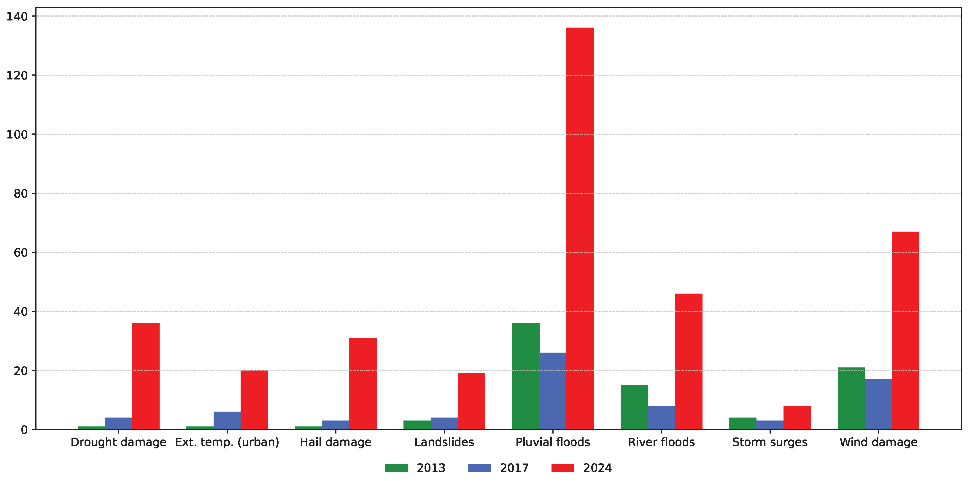
Figure 1. Number of extreme weather events in Italy by type and year, based on data from the LegAmbiente CittàClima map (https://cittaclima.it/mappa/, accessed on 16 April 2025) and elaborated by the authors. All categories refer to 2024, except Ext. temp. (urban) which refers to 2023, since only one event was reported in 2024.
Risks 13 00192 g001
Figure 2. High-resolution spatial grid used for the calculation of ITACI indicators, consisting of 3346 land grid cells covering the Italian territory, extracted from the ERA5-Land dataset. The grid provides the spatial framework on which climatic indicators are computed. The map was produced using the Mercator projection with the Basemap library in Python.
Risks 13 00192 g002
Figure 3. Georeferenced tide gauge stations from the PSMSL RLR dataset, comprising 56 stations selected to compute the sea level indicator. Stations are displayed as black dots and were selected based on geographic coverage and data quality.
Risks 13 00192 g003
Figure 4. Seasonal ITACI values for Italy from 1961 to 2024, calculated according to Formula (5). The five-year moving average is also shown.
Risks 13 00192 g004
Figure 5. Boxplot distributions of national ITACI values by season and multi-year period. Outliers, shown as black open circles, correspond to extreme values beyond 1.5 times the interquartile range.
Risks 13 00192 g005
Figure 6. Spatial distribution of ITACI by season at 0.1° × 0.1° resolution for 2011 (top row) and 2023 (bottom row). Colours represent ITACI values, with positive values indicating above-average climate stress and negative values below-average conditions.
Risks 13 00192 g006
Figure 7. High-resolution spatial grid for the calculation of NUTS1 macro-area indicators, providing the spatial framework for the aggregation of climatic indicators at the NUTS1 level. The map was produced using the Mercator projection with the Basemap library in Python.
Risks 13 00192 g007
Figure 8. ITACI values for the Italian NUTS1 macroareas by season from 1961 to 2024, calculated according to Formula (5) and using the coastline-based weights derived from Table 2. NUTS1 codes are as follows: North-West (ITC), North-East (ITH), Centre (ITI), South (ITF), and Islands (ITG).
Risks 13 00192 g008
Figure 9. Five-year moving averages of the ITACI for Italy and the NUTS1 macro-areas from 1965 to 2024. NUTS1 codes are as follows: North-West (ITC), North-East (ITH), Centre (ITI), South (ITF), and Islands (ITG).
Risks 13 00192 g009
Figure 10. Standardised anomalies of the climatic ITACI components (Warm and Cool Temperatures, Precipitation, Drought, and Wind Power) by season for Italy from 1991 to 2024.
Risks 13 00192 g010
Figure 11. Mean (non-standardised) anomalies of the climatic ITACI components (Warm and Cool Temperatures, Precipitation, Drought, and Wind Power) by season for Italy from 1991 to 2024. Each panel displays the average magnitude and direction of change for each component.
Risks 13 00192 g011
Figure 12. Correlations among monthly values of the national ITACI and its components (Warm and Cool Temperatures, Precipitation, Drought, Wind Power, and Sea Level) over the period 1961–2023. Blue links indicate negative correlations, while red links indicate positive correlations.
Risks 13 00192 g012
Figure 13. Correlations among monthly values of macro-area ITACI and its components (Warm Temperature, Cool Temperature, Precipitation, Drought, Wind Power, and Sea Level) over the period 1961–2023. Blue links indicate negative correlations, while red links indicate positive correlations.
Risks 13 00192 g013
Figure 14. Five-year moving averages of ITACI (Italy) and IACI disaggregated for Spain and Portugal from 1965 to 2023.
Risks 13 00192 g014
Figure 15. Standardised anomalies of Warm Temperature by season for Portugal, Spain, and Italy from 1991 to 2023.
Risks 13 00192 g015aRisks 13 00192 g015b
Figure 16. Five-year moving average of temperature indicators, both disaggregated (Warm Temperature and Cool Temperature) and aggregated (Thermal Component), for Portugal, Spain, and Italy from 1991 to 2023.
Risks 13 00192 g016
Figure 17. Standardised anomalies of Cool Temperature by season for Portugal, Spain, and Italy from 1991 to 2023.
Risks 13 00192 g017aRisks 13 00192 g017b
Figure 18. Standardised anomalies of Precipitation component by season for Portugal, Spain, and Italy from 1991 to 2023.
Risks 13 00192 g018
Figure 19. Five-year moving averages of Precipitation, Drought and Wind Power components for Portugal, Spain, and Italy from 1991 to 2023.
Risks 13 00192 g019
Figure 20. Standardised anomalies of Drought component by season for Portugal, Spain, and Italy from 1991 to 2023.
Risks 13 00192 g020
Figure 21. Standardised anomalies of Wind Power component by season for Portugal, Spain, and Italy from 1991 to 2023.
Risks 13 00192 g021
Figure 22. Five-year moving averages of Sea Level component for Iberian peninsula and Italy from 1991 to 2023.
Risks 13 00192 g022
Figure 23. Seasonal standardised anomalies of Sea Level component for Italy from 1961 to 2023. The five-year moving average is also shown.
Risks 13 00192 g023
Figure 24. Mean (non-standardised) anomalies of the Sea Level component (mm) by season for Italy from 1991 to 2023, showing the average magnitude and direction of change.
Risks 13 00192 g024
Table 1. The indicators used for the calculation of ITACI, including climatic and sea level components, with their symbols, underlying variables, detection criteria, and aggregation rules.
IndicatorSymbol *Variable(s)Detection CriterionAggregation Rule
Warm Days F warm D ( j , ) Max temperature
(6:00 a.m.–6:00 p.m.)
Daytime 90th perc.
(moving window)
Count of daily
exceedances per month
Warm Nights F warm N ( j , ) Max temperature
(7:00 p.m.–5:00 a.m.)
Nighttime 90th perc.
(moving window)
Count of daily
exceedances per month
Cool Days F cool D ( j , ) Min temperature
(6:00 a.m.–6:00 p.m.)
Daytime 10th perc.
(moving window)
Count of daily
exceedances per month
Cool Nights F cool N ( j , ) Min temperature
(7:00 p.m.–5:00 a.m.)
Nighttime 10th perc.
(moving window)
Count of daily
exceedances per month
Precipitation Extremes P max ( j , ) Total daily precipitationNo thresholdMax of 5-day rolling
sums within the month
Drought L dry ( j , ) Total daily precipitation < 1 mmMax dry spell per year,
interpolated monthly
Wind Power F wind ( j , ) Wind components
W E , W N
Daily threshold
( μ + 1.28 σ )
Normalised count of
daily exceedances
Sea Level S ( j , ) Monthly sea levelMean across tide gauge stations
* In the “Symbol” column, j indexes the month and l the year.
Table 2. Italian macroareas A k , with the included regions, NUTS1 codes, coastline lengths, and number of 0.1° × 0.1° land grid cells.
Macro-AreaIncluded RegionsNUTS1
Code
Area
A k
Coastline *
(km)
Cell Nr. **
N k
North-WestPiedmont, Aosta Valley, Liguria, LombardyITC A 1 378716
North-EastTrentino-Alto Adige, Veneto, Friuli-Venezia Giulia, Emilia-RomagnaITH A 2 397704
CentreTuscany, Umbria, Marche, LazioITI A 3 1206653
SouthAbruzzo, Molise, Campania, Apulia, Basilicata, CalabriaITF A 4 2445769
IslandsSicily, SardiniaITG A 5 3754504
* The total Italian coastline length is approximately 7900 km. ** The total number of national grid cells is N = 3346 .
Disclaimer/Publisher’s Note: The statements, opinions and data contained in all publications are solely those of the individual author(s) and contributor(s) and not of MDPI and/or the editor(s). MDPI and/or the editor(s) disclaim responsibility for any injury to people or property resulting from any ideas, methods, instructions or products referred to in the content.