Towards Examining the Volatility of Top Market-Cap Cryptocurrencies Throughout the COVID-19 Outbreak and the Russia–Ukraine War: Empirical Evidence from GARCH-Type Models

Abstract

The cryptocurrency market, known for its inherent volatility, has been significantly influenced by external shocks, particularly during periods of global crises such as the COVID-19 pandemic and the Russia–Ukraine war. This study investigates the volatility of the top seven cryptocurrencies by market capitalization—Bitcoin (BTC), Ethereum (ETH), Tether (USDT), Binance Coin (BNB), USD Coin (USDC), XRP, and Cardano (ADA)—from 1 January 2020 to 1 September 2024, employing a range of GARCH models (GARCH, EGARCH, TGARCH, and DCC-GARCH). This research aims to examine the persistence of leverage effects, volatility asymmetry, and the impact of past price fluctuations on future volatility, with a particular focus on how these dynamics were shaped by the pandemic and geopolitical tensions. The findings reveal that past price fluctuations had a limited impact on future volatility for most cryptocurrencies, although leverage effects became evident during market anomalies. Stablecoins (USDC and USDT) showed a distinct volatility pattern, reflecting their peg to the US Dollar, while platform-associated BNB demonstrated unique volatility characteristics. The results underscore the market’s sensitivity to price movements, highlighting the varying reactions of investor profiles across different cryptocurrencies. These insights contribute to understanding volatility transmission within the cryptocurrency market during times of crisis and offer important implications for market participants, particularly in the context of risk management strategies.

1. Introduction

The global financial landscape has undergone unprecedented disruptions in recent years, primarily due to the COVID-19 pandemic and the Russia–Ukraine war. The COVID-19 outbreak, which emerged in late 2019, triggered a severe economic downturn, leading to heightened uncertainty in financial markets as governments imposed lockdowns, trade restrictions, and fiscal stimulus measures (Baker et al. 2020). Zhang et al. (2023) proved that the volatility in cryptocurrency markets increased significantly following regulatory announcements, particularly from Chinese policymakers, during the pandemic. Ben-Ahmed et al. (2023) found that the volatility increased significantly during the initial phase of the pandemic but did not have a long-term effect. For instance, volatility declined after the World Health Organization (WHO) declared COVID-19 a pandemic on 11 March 2020, suggesting a short-term effect. However, Bentouir et al. (2022) indicated that volatility persisted in the long term, with cryptocurrencies showing high levels of instability, especially in the second half of 2020. Meanwhile, the Russia-Ukraine war, which began in February 2022, further increased commodity volatility, mainly driven by Russia’s foreign exchange reserves, followed by trade, sentiment, and monetary policy, with investor panic and Fed rate hikes amplifying the impact (Fang and Shao 2022). Kamal and Wahlstrøm (2023) reported that the conflict caused a notable drop in both liquidity and returns for cryptocurrencies. These macroeconomic shocks have not only disrupted traditional asset classes but have also raised critical questions about the resilience of cryptocurrencies, which are often perceived as speculative assets with unique risk–return characteristics.

While the volatility of cryptocurrencies has been extensively studied (Baur and Dimpfl 2018; Balcilar et al. 2017; Katsiampa 2017; Katsiampa 2019), existing research has largely focused on structural factors or conventional market conditions. However, little is known about how cryptocurrencies respond to extreme global events such as pandemics and geopolitical conflicts. Prior studies (Urquhart 2016) have either overlooked the role of major exogenous shocks in shaping cryptocurrency volatility or have provided fragmented insights without a systematic examination of their broader implications. This study seeks to fill this gap by offering a comprehensive analysis of cryptocurrency volatility in the context of the COVID-19 pandemic and the Russia–Ukraine war, employing GARCH-type models to assess the persistence, leverage effects, and event-specific volatility shifts in the market.

The novelty of this study lies in its multi-faceted approach to understanding cryptocurrency volatility under extreme uncertainty. Unlike previous studies (Bariviera 2017) that primarily assess volatility trends during normal market conditions, this research explicitly investigates: volatility persistence (whether cryptocurrencies exhibit prolonged high volatility during major events), leverage effects (how negative price shocks disproportionately impact volatility), event-specific volatility (whether the COVID-19 pandemic and the Russia–Ukraine war had asymmetric effects on the cryptocurrency market), as well as stablecoin stability (the effectiveness of stablecoins as risk-hedging instruments during financial crises). By analyzing a portfolio of the top seven cryptocurrencies, this study provides empirical evidence on the resilience of digital assets during major financial disruptions. The findings have significant implications for investors, policymakers, and financial institutions seeking to navigate cryptocurrency markets amid heightened global uncertainty.

The remainder of this paper is structured as follows: Section 2 presents an overview of the cryptocurrency market and a review of prior literature on volatility modeling. Section 3 formulates the research hypotheses. Section 4 details the research methodology, followed by empirical results in Section 5. Section 6 discusses the findings, while the last section concludes with policy implications and directions for future research.

2. Literature Review

2.1. The Transformation of the Cryptocurrency Market: Adoption, Volatility, and Market Behavior

The cryptocurrency market has rapidly evolved into a complex and dynamic financial ecosystem. Between 2020 and 2024, the cryptocurrency market experienced substantial growth in the number of listed digital assets. In 2020, approximately 5000 cryptocurrencies were actively traded, reflecting the ongoing development of blockchain technology and its adoption across various sectors (Cryptomus 2024). By 2024, this number had more than doubled, surpassing 10,000 cryptocurrencies, highlighting the rapid expansion of the market. This growth was driven by innovations in decentralized finance (DeFi), non-fungible tokens (NFTs), and various blockchain-based applications, despite challenges such as regulatory uncertainty and market volatility. The increasing number of cryptocurrencies underscores the dynamic and evolving nature of the digital asset space, as it continues to attract both developers and investors.

During the COVID-19 crash on 13 March 2020, the crypto market experienced its worst single-day correction, dropping 39.6%. Bitcoin fell by 35.2%, while Ethereum saw a 43.1% decline. This dramatic sell-off was driven by global panic and uncertainty, as investors moved away from risk assets. The total crypto market cap fell from USD 223.74 billion to USD 135.14 billion overnight (TheStreet 2025). Following Russia’s invasion of Ukraine, Bitcoin’s price fell below USD 35,000, marking a significant decline. Ethereum (ETH) also experienced a sharp drop, tumbling over 12% (Forbes 2022).

The unique characteristics of Bitcoin have been the subject of extensive research. Studies by Corbet et al. (2018) and Grinberg (2011) highlighted that Bitcoin possesses attributes more akin to an asset class than a conventional currency, offering potential for hedging and risk management. Baur et al. (2018) supported that Bitcoin’s return properties differ significantly from traditional assets, offering substantial diversification benefits in both stable and turbulent periods. These features have positioned Bitcoin as a digital alternative to traditional safe-haven assets like gold. Dwyer (2015) further emphasized Bitcoin’s distinctive nature by demonstrating that its monthly return volatility significantly exceeds that of gold and certain foreign exchange rates against the U.S. dollar. This intensified volatility underscores both the potential rewards and risks associated with Bitcoin as an investment. Wang (2021) found that Bitcoin shows clustering and persistence in returns and volatility, with no “Leverage Effect” concluding it acts as a safe-haven asset for hedging financial risks and is valuable for portfolios. Corbet et al. (2022) showed that cryptocurrencies, amid the COVID-19 pandemic, acted as a potential safe-haven asset, with increased market liquidity and significant interactions between price and liquidity shocks, which intensified during both domestic and international contagion phases, supporting their role as a store of value during financial market panic.

The broader cryptocurrency market, characterized by the proliferation of alternative coins (altcoins) and decentralized financial instruments, continues to attract a diverse range of investors. This market’s rapid expansion, fueled by technological innovation and increasing institutional interest, suggests a transformative impact on global financial systems, warranting ongoing academic exploration.

2.2. Prior Literature Towards Volatility in Cryptocurrencies: Insights from Market Forces, Speculation, and Global Events

The cryptocurrency market is known for its potential for high returns, but this potential comes with a significant degree of volatility—a defining characteristic of the market. Yermack (2013) provided early evidence that cryptocurrencies resemble speculative assets more than traditional currencies, emphasizing their inherent volatility and risk. Further research by Baur et al. (2018) revealed that over 30% of Bitcoin is held purely for investment purposes, with these investors predominantly holding onto their assets rather than engaging in transactions, highlighting the speculative nature of Bitcoin ownership.

Ciaian et al. (2016) demonstrated that Bitcoin price fluctuations are primarily driven by market forces and investor attractiveness, with minimal influence from macroeconomic factors in the long run. Kristoufek (2015) also supported the view that Bitcoin prices are largely driven by speculative investments, further illustrating the asset’s speculative nature. Polasik et al. (2015) added that Bitcoin’s returns are sensitive to both news events and trading volume, indicating that market sentiment and transaction activity play crucial roles in price determination.

The factors influencing cryptocurrency volatility have also been extensively studied. Yi et al. (2018) provided evidence of a spillover effect within the cryptocurrency market, showing that movements in market capitalization significantly impact volatility. Cryptocurrencies with larger market capitalizations, such as Bitcoin, tend to transmit volatility shocks, while those with smaller capitalizations tend to absorb these shocks. Despite Bitcoin’s dominant market position, Ciaian et al. (2018) argued that the prices of certain altcoins are not significantly impacted by Bitcoin’s fluctuations in the long run, suggesting that some cryptocurrencies operate independently of Bitcoin’s influence.

Ciaian et al. (2016) further showed that supply-side factors have a lesser impact on Bitcoin’s price compared to demand-side variables, such as the volume of daily transactions. As the cryptocurrency market continues to grow, understanding these factors becomes increasingly important for predicting market movements. Research by Conrad et al. (2018) explored long-term influences on Bitcoin’s volatility, finding that S&P 500 volatility has a strong negative impact on Bitcoin’s long-term volatility, while the S&P 500 risk premium positively affects it. They also reported a negative correlation between Bitcoin’s price and trading volume.

Aalborg et al. (2019) found that the number of unique addresses used in the Bitcoin network is positively correlated with Bitcoin’s daily returns, suggesting that network activity is a significant driver of price. Moreover, Symitsi and Chalvatzis (2018) identified significant return spillovers from energy and technology stocks to Bitcoin, with short-term volatility spillovers from technology companies affecting Bitcoin, and Bitcoin’s volatility having long-term impacts on energy companies.

In terms of portfolio management, Brière et al. (2015) concluded that including a small allocation of Bitcoin in a well-diversified portfolio could enhance the risk–return profile. However, they cautioned that this benefit might not be sustainable in the medium to long term. Based on the asymmetric GARCH model, Dyhrberg (2016a) demonstrated Bitcoin’s utility in risk management, especially for risk-averse investors during negative market shocks. However, Baur and Dimpfl (2018) highlighted that cryptocurrencies’ volatility increases more in response to positive shocks than negative ones, which contrasts with typical stock market behavior. Further, Dyhrberg (2016b) provided evidence that Bitcoin can serve as a hedge against the U.S. dollar and, to some extent, against stocks in the Financial Times Stock Exchange (FTSE), but only in the short term.

Other research has underscored the significant impact of the COVID-19 pandemic on cryptocurrency volatility and the evolving relationships among major financial assets. Karagiannopoulou et al. (2023) demonstrated that news driven by fear, such as escalating COVID-19 case numbers, notably increased Bitcoin’s volatility. Specifically, the study observed that a shock from COVID-19 cases initially had a strong negative effect on Bitcoin’s volatility, with this impact reaching its peak between 1 and 2.5 days before becoming weakly positive. Salisu and Ogbonna (2022) confirmed that fear-driven news related to the pandemic significantly increased cryptocurrency return volatility compared to the pre-pandemic period

An additional investigation by Yarovaya et al. (2022) assessed whether the COVID-19 pandemic constituted a black swan event for cryptocurrencies, leading to behavioral anomalies such as investor herding. In a similar vein, Conlon and McGee (2020) reported that Bitcoin did not operate as a safe haven asset during the crisis, contradicting its traditional role as a refuge in times of financial instability.

Further, the conflict between Russia and Ukraine has had significant effects on cryptocurrency markets, causing noticeable volatility and changes in liquidity. Theiri et al. (2023) indicated a significant yet temporary increase in liquidity of Bitcoin and Ethereum immediately following the invasion, with levels normalizing shortly thereafter. Long et al. (2022) supported that cryptocurrencies with lower exposure to geopolitical risk tend to deliver better performance than those with higher geopolitical sensitivity. Hampl et al. (2024) suggested that crypto assets demonstrate limited safe-haven characteristics for the commodity market but exhibit robust safe-haven properties for foreign exchange currencies.

2.3. Understanding Cryptocurrency Volatility Through the Lens of GARCH Models

As the cryptocurrency market has evolved, there has been a notable increase in research dedicated to understanding the price dynamics and volatility of digital assets. Among the diverse methodologies employed, GARCH (Generalized Autoregressive Conditional Heteroskedasticity) models have become indispensable tools for estimating time-varying volatility in this market, which is characterized by high uncertainty and rapid price fluctuations. Bouoiyour and Selmi (2015) conducted a comprehensive study on Bitcoin’s price volatility, utilizing various extensions of GARCH models in their quest for the most effective specification. Their findings indicated that Bitcoin’s volatility is highly responsive to negative news, suggesting that adverse information can significantly exacerbate price swings. This sensitivity highlights the critical need to account for news events when modeling and forecasting Bitcoin’s volatility. Using GARCH(1,1) and GJR-GARCH(1,1) models, Khan and Khan (2021) identified volatility clustering and leverage effects in the cryptocurrencies. The results showed that the crypto market experienced volatility persistence, fat-tail phenomena, and leverage effects during the pandemic. Taera et al. (2023) used univariate GARCH models to examine the volatility impact of the COVID-19 pandemic and the Russia–Ukraine war on five asset classes: Islamic, ESG, conventional, crypto, FinTech, and commodities. Their findings revealed that, with the exception of Bitcoin, most assets experienced increased volatility during these crises.

In another approach, Beneki et al. (2019) employed a bivariate diagonal BEKK-GARCH(1,1) model to analyze the volatility dynamics between Bitcoin (BTC) and Ethereum (ETH). This model enabled the simultaneous modeling of both variance and covariance, offering a deeper insight into the interactions between these two major cryptocurrencies. The study further incorporated an impulse response analysis within a Vector Autoregression (VAR) framework, revealing a delayed response in Bitcoin’s volatility following shocks to Ethereum returns. These results suggest inefficiencies in the Bitcoin market, indicating that traders should exercise caution when incorporating highly volatile or interdependent cryptocurrencies into their portfolios.

Katsiampa (2017) examined various GARCH-type models to analyze Bitcoin’s price volatility. The study revealed that the AR-CGARCH model provides the best fit in terms of data accuracy. Furthermore, Katsiampa (2019) used an asymmetric diagonal BEKK model to analyze the volatility dynamics of five major cryptocurrencies: Bitcoin, Ether, Ripple, Litecoin, and Stellar Lumen. The study found that the conditional variances of all five cryptocurrencies are significantly influenced by past squared errors and conditional volatility.

2.4. Earlier Studies on Volatility Dynamics in Cryptocurrencies: GARCH and Emerging Methodologies

A substantial body of literature has focused on applying various GARCH models to capture the volatility dynamics of cryptocurrencies like Bitcoin, Ethereum, and a wide range of other digital currencies.

Chi and Hao (2021) evaluated the effectiveness of different volatility models for Bitcoin (BTC) and Ethereum (ETH). Their study found that the single-variate GARCH model performed well both in-sample and out-of-sample, while the GJR-GARCH model did not show significant asymmetric volatility responses to past returns. Although the multi-variate VARMA-DCC-AGARCH model excelled in-sample, it underperformed out-of-sample compared to the GARCH model. Additionally, GARCH-based volatility forecasts surpassed option-implied volatility, leading to profitable trading strategies by exploiting pricing inefficiencies in the cryptocurrency options market.

Bergsli et al. (2022) focused on forecasting Bitcoin volatility, comparing various GARCH models and heterogeneous autoregressive (HAR) models. The study concluded that EGARCH and APARCH models were the most effective among GARCH variants, while HAR models based on realized variance from high-frequency data outperformed GARCH models that relied on daily data, especially for short-term volatility forecasts.

Tan et al. (2021) proposed a time-varying transition probability Markov-switching GARCH (TV-MSGARCH) model to address Bitcoin’s extreme volatility. Incorporating BTC daily trading volume and Google search data as exogenous variables, this model outperformed traditional GARCH models in in-sample fitting and provided superior out-of-sample forecasts, highlighting the significance of time-varying effects in transition probabilities.

Apergis (2022) examined the impact of the COVID-19 pandemic on the conditional volatility of returns for eight cryptocurrencies using an asymmetric GARCH modeling approach. The study found that the pandemic positively influenced conditional volatility and incorporating it as an explicit factor improved the accuracy of volatility forecasts.

Kyriazis et al. (2019) explored the volatility of several cryptocurrencies during the bearish market of 2018, focusing on the influence of Bitcoin, Ethereum, and Ripple—three of the highest capitalization digital currencies. Using ARCH, GARCH, and DCC-GARCH models, the study concluded that most cryptocurrencies were complementary to Bitcoin, Ethereum, and Ripple, with no significant hedging abilities observed among these major digital currencies during market downturns.

Fung et al. (2022) analyzed the risk and return characteristics of 254 diverse cryptocurrencies, focusing on traded volume and primary usage. The study revealed common features such as long memory, volatility clustering, heavy tails, and negative leverage effects. GARCH models accounting for these features, particularly Student’s -distribution GARCH specifications, provided the best fit for about 80% of cryptocurrencies studied, with TGARCH-stud being optimal for 20% of the sample. Out-of-sample 1%-Value-at-Risk (VaR) forecasts using heavy-tailed distributions outperformed those based on normal distributions. Caporale and Zekokh (2019) highlighted that two-regime GARCH models outperform single-regime ones in predicting VaR and Expected Shortfall (ES) for major cryptocurrencies, highlighting significant leverage effects and the need for regime-switching frameworks to improve risk management and regulatory oversight. According to Chu et al. (2017), IGARCH and GJRGARCH effectively model cryptocurrency volatility, underscoring the need for deeper analysis, regulatory oversight, and improved risk measures. Klein et al. (2018) revisits Bitcoin return volatility modeling using GARCH-class models, finding that the Fractionally Integrated APARCH (FIAPARCH) model provides the best fit, indicating Bitcoin’s asymmetric response to market shocks and high volatility persistence, with similar behavior observed in other cryptocurrencies.

Hattori (2020) evaluated volatility modeling in the Bitcoin market using realized volatility as a reliable proxy for true volatility, calculated from 5 min intraday returns. The study assessed model performance through MSE and QLIKE metrics, ensuring forecast accuracy despite potential noise in the volatility proxy. The findings indicated that asymmetric volatility models like EGARCH and APARCH demonstrated higher predictability, with models using normal distribution outperforming those with fat-tailed distributions, such as the skewed t-distribution.

Kim et al. (2021) analyzed the volatility of nine leading cryptocurrencies, including Bitcoin, Ethereum, and XRP, using both Bayesian Stochastic Volatility (SV) and several GARCH models. The study found that the SV model outperformed GARCH models, particularly with highly volatile financial data like cryptocurrencies. The SV model’s forecasting errors were more accurate than those of GARCH models, especially over longer forecast horizons, offering deeper insights into volatility forecasting in the complex cryptocurrency market.

Pratas et al. (2024) compared the forecasting abilities of classic GARCH models with deep learning methodologies, including MLP, RNN, and LSTM architectures, for predicting Bitcoin’s volatility. Analyzing Bitcoin logarithmic returns from 2014 to 2022, the study found that deep learning models offered superior forecast quality, although with significant computational costs. While MLP and RNN models produced smoother forecasts but missed large volatility spikes, the LSTM model effectively captured and adjusted to such movements. The study confirmed the superiority of deep learning methodologies, particularly for short-term forecasts, suggesting their potential as powerful tools for predicting Bitcoin returns and volatility.

Yıldırım and Bekun (2023) examined the prediction of Bitcoin’s return volatility using weekly Bitcoin price data from 2013 to 2020. They identified the best-fitting model through the Akaike information criterion, finding that the GARCH(1,1) model was most suitable, though the ARCH-LM test indicated no ARCH effect in the residuals.

Tiwari et al. (2019) compared various GARCH and stochastic volatility (SV) models to assess their fit for Bitcoin and Litecoin price returns. The study evaluated models including GARCH(1,1), SV with AR(1) log-volatility, and more flexible models incorporating jumps, leverage effects, and t-distributed innovations. The findings indicated that the SV-t model was best suited for Bitcoin, while the GARCH-t model performed best for Litecoin. Overall, t-distributed models outperformed others for both cryptocurrencies, and SV models consistently outperformed GARCH models.

Ferreira et al. (2024) examined the volatility of four cryptocurrencies—MATIC, SOL, BTT, and VET—using GARCH, EGARCH, and TGARCH models to determine the optimal model for each. The study found that EGARCH(1,1) was best for MATIC, while GARCH(1,1) suited VET. However, for SOL and BTT, the models failed to meet necessary assumptions, indicating that GARCH models may not be suitable for these cryptocurrencies. This research highlights the varying effectiveness of volatility models across different cryptocurrencies with limited market presence compared to Bitcoin.

The reviewed studies highlight the diverse approaches taken to model and forecast cryptocurrency volatility, with GARCH models playing a central role. While GARCH models often provide good fit and predictive power, particularly for major cryptocurrencies like Bitcoin and Ethereum, alternative models like stochastic volatility (SV) and deep learning methods are increasingly showing superior performance, especially in more volatile or less liquid markets. The choice of the optimal model is highly context-dependent, influenced by factors such as the specific cryptocurrency being analyzed, the time horizon, and the nature of the data.

3. Research Hypotheses

Cryptocurrency markets, particularly Bitcoin (BTC), Ethereum (ETH), Cardano (ADA), and Ripple (XRP), are notorious for their high volatility. This volatility tends to persist, with periods of heightened volatility often followed by other volatile periods, especially during financial uncertainty caused by major economic and geopolitical shocks. Given the speculative nature and market depth of cryptocurrencies, understanding these volatility dynamics during extreme events like the COVID-19 pandemic and the Russia–Ukraine war is essential for assessing their resilience in the face of major global disruptions. Assaf et al. (2022) found that most cryptocurrencies showed a downward trend in persistence after the 2017 bubble, followed by a sharp decline after the COVID-19 outbreak. However, Dash was an exception, showing low persistence before COVID-19 and a shift to high persistence afterward. Therefore, the Volatility Dynamics Hypothesis is formulated as follows:

H1.1. 

The volatility of major cryptocurrencies does not exhibit persistent effects during periods of financial uncertainty.

H1.2. 

The volatility of major cryptocurrencies exhibits persistent effects during periods of financial uncertainty, as indicated by GARCH models.

In the cryptocurrency market, leverage effects can be amplified due to speculative trading, high investor sentiment, and the use of leverage in trading. During periods of extreme stress, such as the COVID-19 pandemic and the Russia–Ukraine war, these leverage effects may become more pronounced, leading to disproportionate price swings. Negative shocks, especially in volatile markets like cryptocurrencies, tend to amplify volatility, triggering sell-offs and forced liquidations. Huang et al. (2022) found that Bitcoin and Ethereum demonstrate differing leverage effects, with Bitcoin experiencing a shift from a negative to a positive relationship, while Ethereum shows a strong generalized leverage effect. However, according to Brini and Lenz (2022), the absence of a leverage effect in the cryptocurrency market is attributed to the fact that many investors enter the market without a deep understanding of the asset class, often driven by the low barrier to entry, the disruptive potential of cryptocurrencies, and the underlying blockchain technology. Hence, the Leverage Effects Hypothesis is framed as below:

H2.1. 

Negative price shocks do not disproportionately amplify volatility in major cryptocurrencies.

H2.2. 

Negative price shocks disproportionately amplify volatility in major cryptocurrencies, confirming the presence of leverage effects.

Both the COVID-19 pandemic and the Russia–Ukraine war introduced significant market uncertainty, though each event had different financial consequences. The pandemic, a global economic shock, caused widespread market panic and triggered a global recession. In contrast, the Russia–Ukraine war, while a geopolitical crisis, initially had more localized market effects, especially in energy markets and global trade. The hypothesis is based on the assumption that the nature and scope of these events would affect cryptocurrencies differently. Foroutan and Lahmiri (2022) examined the effects of the COVID-19 pandemic on the return–volatility and return–volume relationships for the ten most traded cryptocurrencies, comparing them with less volatile markets such as gold and crude oil. Their findings show that the return–volatility relationship became significant for several cryptocurrencies during the pandemic, whereas it was not significant before, and that trading volume exhibited causal relationships with returns for certain cryptocurrencies during the pandemic. Thus, the Event-Specific Volatility Hypothesis is formulated as follows:

H3.1. 

The COVID-19 pandemic and the Russia–Ukraine war had an equal impact on cryptocurrency volatility.

H3.2. 

The COVID-19 pandemic had a stronger impact on cryptocurrency volatility than the Russia–Ukraine war.

Stablecoins, such as USDC and USDT, are designed to maintain price stability by being pegged to fiat currencies like the U.S. dollar. During times of market turmoil, stablecoins are expected to perform better than other cryptocurrencies, providing a safe haven for investors. Given their fixed value, stablecoins should exhibit less volatility during major crises such as the COVID-19 pandemic and the Russia–Ukraine war. James et al. (2021) highlighted anomalies in the extreme and erratic behavior of cryptocurrencies, particularly with USDT and TUSD, which exhibited unusually stable profiles. This stability is likely attributed to their thin trading structures and limited market liquidity, making them less prone to extreme fluctuations compared to other cryptocurrencies. Hence, the Stablecoin Stability Hypothesis is formulated as below:

H4.1. 

Stablecoins do not serve as effective risk-hedging instruments during financial crises.

H4.2. 

Stablecoins serve as effective risk-hedging instruments during financial crises, maintaining relative stability.

4. Empirical Methodology

4.1. Selected Data

For this research, we selected the top seven digital assets by market capitalization—Bitcoin (BTC), Ethereum (ETH), Tether (USDT), BNB (BNB), USDC (USDC), XRP (XRP), and Cardano (ADA)—for the period from 1 January 2020 to 1 September 2024, covering the COVID-19 outbreak and the Russia–Ukraine war. The sample encompasses a range of digital assets as described in

Table 1. Description of the top seven selected digital assets by market capitalization.

Digital Asset	Abbreviation	Description
Bitcoin	BTC	The world’s first decentralized digital currency, introduced in 2009 by an anonymous person or group using the pseudonym Satoshi Nakamoto. It operates on a peer-to-peer network without the need for intermediaries like banks or governments. Satoshi (2008) argued that a peer-to-peer electronic cash system enables direct online payments between parties without the need for a financial institution. Transactions are verified by network nodes through cryptography and recorded on a public, immutable blockchain ledger.
Ethereum	ETH	A decentralized, open-source blockchain platform that enables the creation of smart contracts and decentralized applications (DApps). It was proposed in 2013 by Vitalik Buterin and launched in 2015. Unlike Bitcoin, which primarily serves as a digital currency, Ethereum is designed to be a programmable blockchain that supports a wide range of applications, including DeFi (Decentralized Finance), NFTs (Non-Fungible Tokens), and DAOs (Decentralized Autonomous Organizations).
Tether	USDT	A stablecoin that is pegged to the value of the U.S. dollar (USD) on a 1:1 basis. It was launched in 2014 by the company Tether Limited and operates on multiple blockchain networks. USDT is designed to provide the stability of fiat currency while maintaining the efficiency and transparency of blockchain technology.
BNB	BNB	The native cryptocurrency of the Binance ecosystem, originally launched in 2017 as an ERC-20 token on the Ethereum blockchain. Later, it migrated to its own blockchain, the BNB Chain (formerly Binance Smart Chain and Binance Chain). BNB was created by Binance, one of the world’s largest cryptocurrency exchanges, to be used for transaction fees, trading, and various applications within the Binance ecosystem.
USDC	USDC	A stablecoin pegged to the U.S. dollar (USD) at a 1:1 ratio. It was launched in 2018 by Circle in partnership with Coinbase, operating under the Centre Consortium. USDC is backed by fiat reserves, including cash and short-term U.S. government bonds, making it a reliable digital equivalent of the dollar. It is widely used in decentralized finance (DeFi), cross-border payments, and cryptocurrency trading.
XRP	XRP	A digital asset and the native cryptocurrency of the XRP Ledger (XRPL), an open-source, decentralized blockchain designed for fast and efficient cross-border payments. It was created in 2012 by Ripple Labs (San Francisco, CA, USA) to facilitate instant, low-cost international transactions for banks, financial institutions, and payment providers. Unlike Bitcoin and Ethereum, XRP does not rely on mining; instead, it uses a unique consensus mechanism for transaction validation.
Cardano	ADA	A decentralized, open-source blockchain platform designed for scalability, security, and sustainability. It was founded in 2017 by Charles Hoskinson, one of the co-founders of Ethereum, and is developed by Input Output Global (IOG). Cardano aims to improve upon previous blockchain networks by using a scientific, research-driven approach to development.

: cryptocurrencies, which are decentralized digital currencies using blockchain technology; tokens, which are assets issued on existing blockchains often representing specific rights or assets; and stablecoins, which are tokens designed to maintain a stable value by being pegged to fiat currencies or other assets.

A dummy variable, referred to as “COVID-19” was incorporated to capture the impact of the COVID-19 pandemic. This variable was assigned a value of 1 for the period from 11 March 2020, when the World Health Organization (WHO) officially declared COVID-19 a global pandemic, to 5 May 2023, when the WHO declared the end of the pandemic as a global health emergency. For all other periods, the variable was set to 0. Furthermore, another dummy variable, labeled “WAR” was introduced to account for the Russia–Ukraine war. This variable was assigned a value of 1 from 24 February 2022, the date marking the beginning of the conflict, until 1 September 2024, which represents the end of the sample period. In all other cases, the variable was assigned a value of 0.

Table 2. Price of the top seven cryptocurrencies by market capitalization throughout major events.

Date Meaning	Price (USD)	BTC	ETH	XRP	BNB	USDC	USDT	ADA
		Type
		Cryptocurrency	Token	Cryptocurrency	Cryptocurrency	Stablecoin	Stablecoin	Cryptocurrency
Onset of the sample	1 January 2020	29,260	730	0.238	14	1.0041	0.99984	0.0335
WHO declaration of COVID-19	11 March 2020	7859	193	0.207	17	0.9973	0.99881	0.0396
Commencement of the Russia–Ukraine war	24 February 2022	38,400	2636	0.703	361	1.0000	1.00064	0.8534
WHO officially declared the end of COVID-19 as a global health emergency	5 May 2023	29,525	1990	0.467	327	1.0000	1.00102	0.3947
End of the sample	1 September 2024	58,419	2502	0.5600	513	1.0000	1.0000	0.3317

shows the price in USD of the top seven cryptocurrencies by market capitalization, selected for this study. We can observe that all cryptocurrencies and tokens selected have significant price changes throughout the major events considered. USDC and USDT maintain their price as they are stablecoins and are capped to the US Dollar.

The data consists of daily (1705 days) observations. The main source of the cryptocurrencies’ daily closing price was coinmarketcap.com. Log returns were computed using Equation (1) in line with Urquhart (2016), Bariviera (2017), and James et al. (2021).

$$r_{i,t}=\mathrm{l}\mathrm{o}\mathrm{g}\hspace{0.17em}\left({\displaystyle \frac{P_{i,t}}{P_{i,t-1}}}\right)$$

(1)

where $P_{i,t}$ is the price of cycryptocurrency at time t and $r_{i,t}$ is the individual daily return of cryptocurrency i at time t.

A crypto index (CC7) was also designed, being computed throughout Equation (2) of the top 7 individual samples, to also have an overall view of the market.

$$r_{m,t}={\displaystyle \frac{{\sum }_{i=1}^N{r}_{i,t}}{N}}$$

(2)

where $r_{m,t}$ is the market return at time t, calculated as a weighted average of the sum of the daily individual returns $r_{i,t}$ at time t and N = 7 being the number of cryptocurrencies in this research.

4.2. Quantitative Framework

4.2.1. ARCH Model Framework

The returns of cryptocurrency $r_{i,t}$ (for each individual digital asset $i$) are typically modeled as a linear function of past returns (for the mean equation) and past volatility (for the variance equation). The general form for the mean equation is presented below:

$$r_{i,t}={\mu }_i+{ϵ}_{i,t}$$

(3)

where $r_{i,t}$ is the log return of cryptocurrency $i$ at time $t$, ${\mu }_i$ denotes the constant mean return for cryptocurrency $i$, and ${ϵ}_{i,t}$ is the error term or residual at time $t$, which is assumed to have conditional variance $h_{i,t}$.

The residuals ${ϵ}_{i,t}$ are assumed to follow a conditional normal distribution with a mean of zero and a variance of $h_{i,t}$. The variance $h_{i,t}$ (conditional volatility) is modeled using the ARCH (Autoregressive Conditional Heteroskedasticity) structure as follows:

$${ϵ}_{i,t}={\sigma }_{i,t}{z}_{i,t}$$

(4)

where ${\sigma }_{i,t}^2$ is the conditional variance (volatility) of cryptocurrency $i$ at time $t$ and $z_{i,t}$ is the standardized error term, assumed to be i.i.d. (independent and identically distributed) with a mean of zero and a unit variance.

The ARCH model assumes that the variance of the error term follows a linear function of past squared residuals. A basic ARCH(1) model for each cryptocurrency $i$ could be written as below:

$$h_{i,t}={\alpha }_0+{\alpha }_1{ϵ}_{i,t-1}^2$$

(5)

where $h_{i,t}$ is the conditional variance (volatility) of cryptocurrency $i$ at time $t$, ${\alpha }_0$ is the constant term (intercept), ${\alpha }_1$ is the coefficient capturing the effect of past squared residuals on current volatility, while ${ϵ}_{i,t-1}^2$ is the squared error term from the previous period.

To account for significant events such as the COVID-19 pandemic and the Russia–Ukraine war, the adjusted model for volatility is presented as follows:

$$h_{i,t}={\alpha }_0+{\alpha }_1{ϵ}_{i,t-1}^2+{\beta }_1{\mathrm{COVID}\text{-}19}_t+{\beta }_2{\mathrm{WAR}}_t$$

(6)

where ${\mathrm{COVID}\text{-}19}_t$ and ${\mathrm{WAR}}_t$ are dummy variables for the COVID-19 pandemic and the Russia–Ukraine war, respectively. ${\beta }_1$ and ${\beta }_2$ capture the impact of these events on the conditional variance.

4.2.2. GARCH(1,1) Model Framework

Engle and Bollerslev (1986) contributed significantly to volatility modeling by extending the ARCH framework to the GARCH model, which remains widely used in financial econometrics, while Nelson (1990) established the conditions for stationarity and ergodicity of the GARCH(1,1) process. However, according to Nelson (1991), GARCH models face three main issues in asset pricing: they ignore the negative correlation between current returns and future volatility, impose restrictive parameter assumptions, and complicate the interpretation of volatility persistence. To capture the potential volatility dynamics in the returns of digital assets, we extend the standard GARCH(1,1) (Generalized AutoRegressive Conditional Heteroskedasticity) model by incorporating two key dummy variables: COVID-19 and WAR. These variables are designed to account for the impact of significant global events on the market behavior of cryptocurrencies. In this regard, the GARCH(1,1) model is specified as follows:

With respect to the mean equation, the return of digital asset $i$ at time $t$, denoted as $r_{i,t}$, is exhibited as follows:

$$r_{i,t}=\mu +{\gamma }_1{\mathrm{COVID}\text{-}19}_t+{\gamma }_2{\mathrm{WAR}}_t+{ϵ}_{i,t}$$

(7)

where $r_{i,t}$ is the log return of cryptocurrency $i$ at time $t$, $\mu$ represents the mean return (assumed to be constant), ${\mathrm{COVID}\text{-}19}_t$ is the dummy variable related to the COVID-19 pandemic, ${\mathrm{WAR}}_t$ is the dummy variable related to the Russia–Ukraine war, ${\gamma }_1$ and ${\gamma }_2$ are the coefficients that capture the effect of the COVID-19 pandemic and the war on the mean returns, and ${ϵ}_{i,t}$ is the innovation or shock term, which is assumed to follow a conditional distribution.

Further, with reference to the variance equation (conditional volatility), the conditional variance of $r_{i,t}$ denoted as ${\sigma }_{i,t}^2$ is modeled as follows:

$${\sigma }_{i,t}^2={\alpha }_0+{\alpha }_1{ϵ}_{i,t-1}^2+{\beta }_1{\sigma }_{i,t-1}^2+{\delta }_1{\mathrm{COVID}\text{-}19}_t+{\delta }_2{\mathrm{WAR}}_t$$

(8)

where ${\sigma }_{i,t}^2$ is the conditional variance (volatility) of asset $i$ at time $t$, ${\alpha }_0$ is the constant term, ${\alpha }_1$ is the coefficient for the lagged squared residual ${ϵ}_{i,t-1}^2$, capturing the past shocks to the market, ${\beta }_1$ is the coefficient for the lagged conditional variance ${\sigma }_{i,t-1}^2$, capturing the persistence of volatility over time, while ${\delta }_1$ and ${\delta }_2$ are the coefficients that capture the impact of the COVID-19 pandemic and the war on the conditional variance (volatility) of the returns.

4.2.3. EGARCH(1,1) Model Framework

The EGARCH(1,1) (Exponential GARCH) conditional variance equation with dummy variables related to the COVID-19 pandemic and Russia–Ukraine war is presented as below:

$$\log \hspace{0.17em}\left({\sigma }_{i,t}^2\right)=\omega +{\alpha }_1\left({\displaystyle \frac{{\epsilon }_{i,t-1}}{{\sigma }_{i,t-1}}}\right)+{\beta }_1\log \hspace{0.17em}\left({\sigma }_{i,t-1}^2\right)+{\gamma }_1\mathrm{C}\mathrm{O}\mathrm{V}\mathrm{I}\mathrm{D}\text{-}{19}_t+{\gamma }_{2}WA{R}_t$$

(9)

where $\log \hspace{0.17em}\left({\sigma }_{i,t}^2\right)$ is the logarithm of the conditional variance of asset $i$ at time $t$, ${\epsilon }_{i,t-1}$ is the lagged error term (innovation), ${\sigma }_{i,t-1}^2$ is the lagged conditional variance, $\omega$ is the constant term, ${\alpha }_1$ captures the impact of past shocks on the current conditional variance, ${\beta }_1$ represents the persistence of volatility from previous periods, ${\gamma }_1$ is the coefficient for the COVID-19 dummy variable, and ${\gamma }_2$ is the coefficient for the WAR dummy variable. ${\gamma }_1$ captures the effect of the COVID-19 pandemic on the conditional volatility of the asset. A positive value suggests that volatility increased during the pandemic period. Likewise, ${\gamma }_2$ captures the effect of the Russia–Ukraine war on the conditional volatility. A positive value would indicate that the war period increased volatility.

4.2.4. TGARCH(1,1) Model Framework

To account for the impact of COVID-19 and the Russia–Ukraine war, we introduce two dummy variables in the conditional variance equation. Hence, the modified conditional variance equation of the TGARCH(1,1) model (threshold GARCH) is presented below:

$${\sigma }_{i,t}^2={\omega }_i+{\alpha }_i{ϵ}_{i,t-1}^2+{\beta }_i{\sigma }_{i,t-1}^2+{\gamma }_i{I}_{\mathrm{negative}}{ϵ}_{i,t-1}^2+{\delta }_{\mathrm{COVID}\text{-}19}{D}_{\mathrm{COVID}\text{-}19,t}+{\delta }_{\mathrm{WAR}}{D}_{\mathrm{WAR},t}$$

(10)

where $D_{\mathrm{COVID}\text{-}19,t}$ is the dummy variable for the COVID-19 pandemic, $D_{\mathrm{WAR},t}$ is the dummy variable for the Russia–Ukraine war, and ${\delta }_{\mathrm{COVID}\text{-}19}$ and ${\delta }_{\mathrm{WAR}}$ are the coefficients capturing the impact of COVID-19 and the Russia–Ukraine war on the volatility.

4.2.5. DCC GARCH(1,1) Model Framework

The return equation for each cryptocurrency $i$ is presented as follows:

$$r_{i,t}={\mathsf{\mu }}_i+{\mathsf{ϵ}}_{i,t}$$

(11)

where $r_{i,t}$ is the log return of cryptocurrency $i$ at time $t$, ${\mu }_i$ denotes the constant mean return for cryptocurrency $i$, and ${ϵ}_{i,t}$ is the error term or residual at time $t$.

The error term ${\mathsf{ϵ}}_{i,t}$ is modeled as below:

$${\mathsf{ϵ}}_{i,t}={\sigma }_{i,t}{z}_{i,t}$$

(12)

where ${\sigma }_{i,t}$ is the conditional volatility at time $t$ and $z_{i,t}\sim \mathcal{N}\left(\mathrm{0,1}\right)$ is the standard normal innovation.

For each cryptocurrency $i$, the conditional volatility ${\sigma }_{i,t}^2$ is modeled using a univariate GARCH(1,1) model:

$${\sigma }_{i,t}^2={\alpha }_i+{\beta }_i{\mathsf{ϵ}}_{i,t-1}^2+{\gamma }_i{\mathsf{\sigma }}_{i,t-1}^2+{\delta }_i{D}_{COVID-19,t}+{\theta }_i{D}_{WAR,t}$$

(13)

where ${\alpha }_i,{\beta }_i, \mathrm{a}\mathrm{n}\mathrm{d} {\gamma }_i$ are the parameters to be estimated for the GARCH model, $D_{COVID-19,t}$ and $D_{WAR,t}$ are the dummy variables for the COVID-19 pandemic and the Russia–Ukraine war, respectively, at time t, and ${\delta }_i$ and ${\theta }_i$ are the coefficients representing the impact of the COVID-19 and WAR events on volatility.

The conditional covariance $\left(\mathrm{Cov}\left(r_{i,t},r_{j,t}\right)\right)$ between two cryptocurrencies $i$ and $j$ is modeled using the DCC framework, which specifies the correlation structure of the multivariate model. The DCC model assumes that the conditional covariance matrix $\left(H_t\right)$ is as follows:

$$H_t=Q_t{D_t}^{-1/2}{R}_t{D_t}^{-1/2}{Q}_t$$

(14)

where $Q_t$ is the time-varying covariance matrix of residuals and $D_{\mathrm{t}}$ is a diagonal matrix of time-varying standard deviations of the individual assets $\left({\sigma }_{i,t}\right)$. $R_{\mathrm{t}}$ is the conditional correlation matrix, which is dynamic and is modeled as follows:

$$R_t=\left(1-{\mathsf{\alpha }}_R-{\beta }_R\right)R_0+{\mathsf{\alpha }}_R\left({\displaystyle \frac{z_{i,t}{z}_{i,t}^{\prime }}{z_{i,t-1}{z}_{i,t-1}^{\prime }}}\right)+{\beta }_R{R}_{t-1}$$

(15)

where $R_0$ is the unconditional correlation matrix, while ${\alpha }_R$ and ${\beta }_R$ are the parameters for the dynamic correlation process.

5. Empirical Results

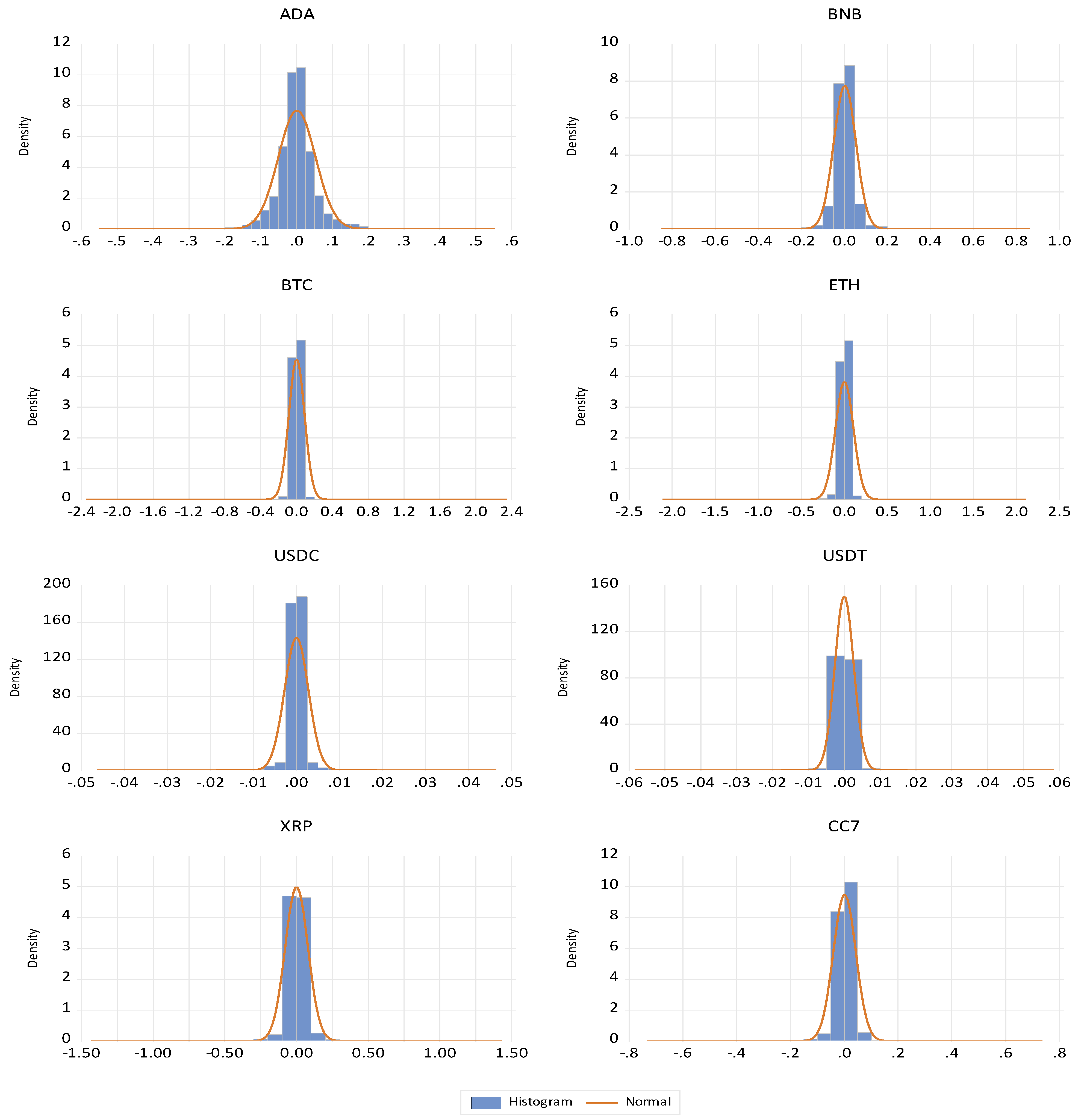
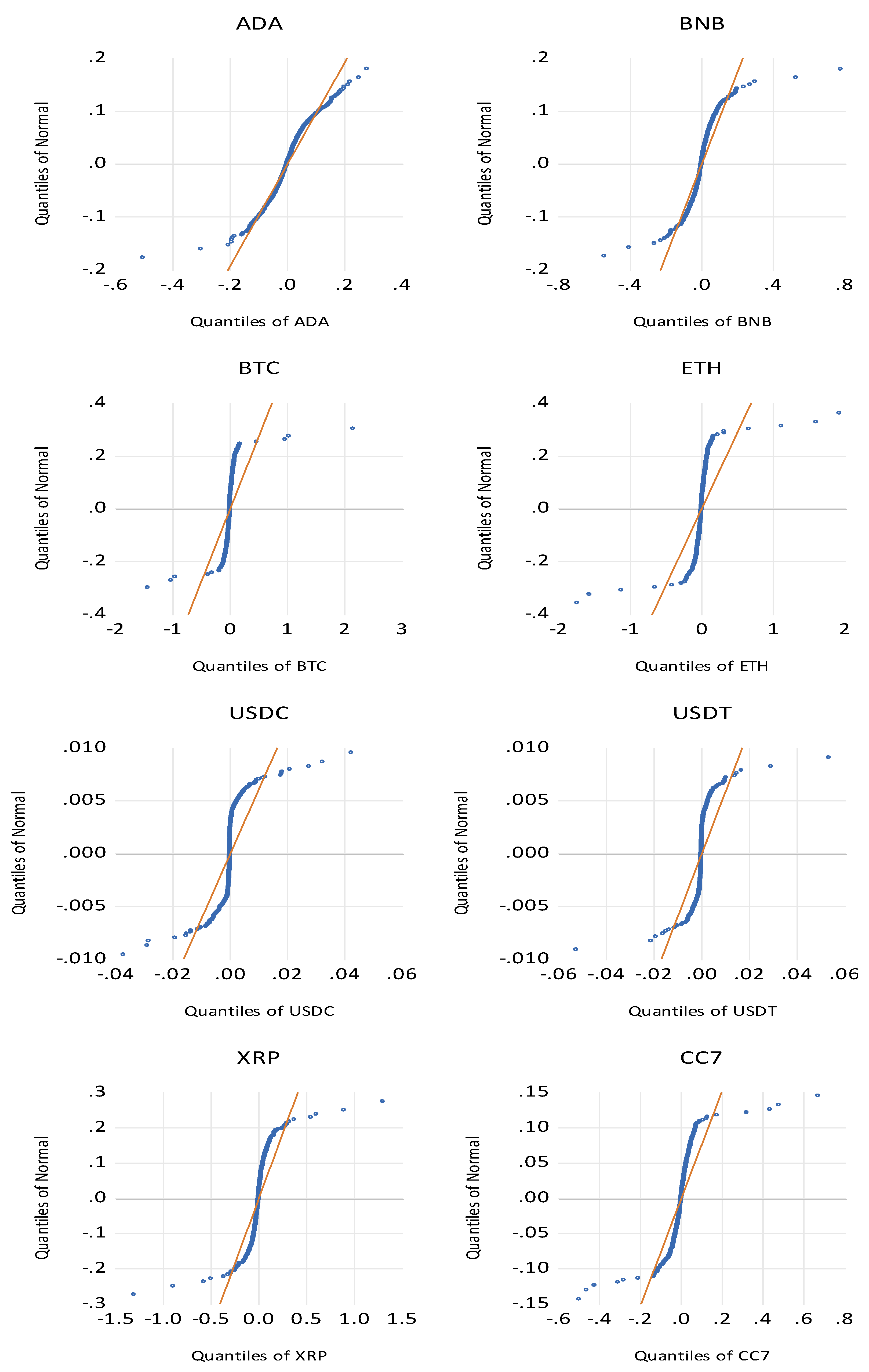
5.1. Descriptive Statistics

The individual descriptive statistics of the log-returns presented in

Table 3. Summary statistics of the top 7 cryptocurrency log returns and CC7.

	ADA	BNB	BTC	ETH	USDC	USDT	XRP	CC7
Mean	0.001265	0.002583	0.001665	0.001856	−7.28E-06	−3.79E-06	0.000501	0.001123
Median	0.000442	0.001398	0.000888	0.001739	2.00E-06	−6.00E-06	−0.00014	0.001875
Maximum	0.279436	0.780889	2.147523	1.931678	0.042439	0.053393	1.304429	0.672576
Minimum	−0.50364	−0.54281	−1.43616	−1.73876	−0.03723	−0.05257	−1.30652	−0.49785
Std. Dev.	0.051889	0.051413	0.087432	0.104477	0.00278	0.002641	0.079804	0.042004
Skewness	−0.22739	1.81669	6.087529	1.088167	1.16401	0.554669	0.086384	1.244048
Kurtosis	11.13653	51.81022	296.5039	194.2136	90.67	208.7554	110.7716	87.92355
Jarque–Bera	4717.871	170,190.2	6,130,383	2,597,807	546,413.4	3,007,656	825,131.3	512,792.9
Probability	0.000000	0.000000	0.000000	0.000000	0.000000	0.000000	0.000000	0.000000
Observations	1705	1705	1705	1705	1705	1705	1705	1705

indicate that all sampled cryptocurrencies exhibit leptokurtic distributions, meaning their return distributions are more peaked and have heavier tails compared to a normal distribution. This suggests frequent extreme movements in prices, which is characteristic of financial assets with high volatility. Examining skewness, ADA, BNB, and ETH display left-skewed distributions, indicating a tendency toward larger negative returns, while BTC, USDC, USDT, and XRP exhibit right-skewed distributions, meaning they experience relatively more frequent large positive returns. Notably, BTC has the highest positive skewness (6.0875), indicating extreme right-tail behavior. Additionally, all selected cryptocurrencies exhibit both positive maximum values and negative minimum values, reinforcing evidence of volatility in each asset throughout the sample period. The market return index (CC7), which aggregates the performance of the top 7 cryptocurrencies, exhibits a left-skewed and leptokurtic distribution, implying that the overall market tends to experience stronger downward price movements than upward ones. Furthermore, Figure A2 confirms that the log returns of all cryptocurrencies and the CC7 deviate significantly from a normal distribution, supporting the rejection of normality.

The daily log-returns presented in Figure 1 exhibit clear evidence of volatility clustering, particularly in ADA, BNB, and CC7, where periods of high volatility are followed by further high volatility, and periods of low volatility persist. Compared to previous studies, such as Bariviera (2017), who identified volatility clustering as a prominent characteristic of Bitcoin, these findings suggest that while BTC exhibits significant volatility, its clustering behavior appears less persistent than that of ADA, BNB, and CC7. This discrepancy may stem from evolving market dynamics, increased institutional adoption, or different modeling periods.

The covariance and correlation matrix in

Table 4. Covariance and correlations of top 7 cryptocurrency log returns and CC7.

Covariance	ADA	BNB	BTC	ETH	USDC	USDT	XRP	CC7
ADA	0.002691
BNB	0.001531	0.002642
BTC	0.000840	0.002014	0.007640
ETH	0.001239	0.002267	0.008068	0.010909
USDC	−9.41E-06	−1.56E-05	−1.29E-05	−1.60E-05	7.72E-06
USDT	−1.85E-05	−2.27E-05	−1.41E-05	−1.76E-05	5.38E-06	6.97E-06
XRP	0.001451	0.001277	0.003700	0.005815	−4.29E-06	−5.41E-06	0.006365
CC7	0.001103	0.001385	0.003176	0.004038	−6.45E-06	−9.41E-06	0.002657	0.001763
Correlation	ADA	BNB	BTC	ETH	USDC	USDT	XRP	CC7
ADA	1.000000
BNB	0.574123	1.000000
BTC	0.185249	0.448377	1.000000
ETH	0.228708	0.422240	0.883799	1.000000
USDC	−0.065253	−0.109378	−0.053134	−0.055296	1.000000
USDT	−0.134843	−0.167139	−0.061049	−0.063768	0.733904	1.000000
XRP	0.350640	0.311444	0.530526	0.697901	−0.019356	−0.025702	1.000000
CC7	0.506554	0.641528	0.865425	0.920644	−0.055298	−0.084890	0.793073	1.000000

suggests the presence of strong positive relationships among certain assets, particularly BTC and ETH (0.8838)—indicating a high degree of co-movement, likely due to their dominance in the market and shared investor sentiment, as well as USDC and USDT (0.7339)—reflecting the fact that both are stablecoins pegged to the U.S. dollar, causing their price movements to be highly synchronized. The correlation between other cryptocurrencies varies, with XRP showing moderate correlations with BTC (0.5305) and ETH (0.6979), while ADA and BNB exhibit lower correlations with BTC and ETH. The CC7 index maintains high correlations with major assets, reinforcing its role as a broad market representative.

The results of the estimated autocorrelation (AC), partial autocorrelation (PAC), and Q-statistics with 36 lags for daily individual log-returns are presented in

Table 5. Estimated autocorrelation (AC), partial autocorrelation (PAC), and Q-statistics with 36 lags for daily individual log-returns.

Variables	Lag Number	AC	PAC	Q-Stat	Prob
ADA	36	−0.0430	−0.0420	74.5000	0.0000
BNB	36	0.0070	0.0030	73.6710	0.0000
BTC	36	0.0020	0.0100	298.8900	0.0000
ETH	36	−0.0030	0.0080	307.5800	0.0000
USDC	36	0.1790	0.0620	736.9900	0.0000
USDT	36	0.1360	0.0060	807.1100	0.0000
XRP	36	−0.0470	−0.0450	185.6600	0.0000
CC7	36	−0.0160	−0.0010	186.0200	0.0000

. The correlogram analysis reveals statistically significant autocorrelations across all cryptocurrencies (p-value = 0.0000). USDC and USDT exhibit moderate positive autocorrelations at lag 36 (0.179 and 0.136, respectively), suggesting a more predictable return behavior compared to other assets. This stability aligns with their function as stablecoins. ADA, XRP, and CC7 show weak negative autocorrelations, indicating a tendency for small reversals in their price movements over time. BTC, BNB, and ETH display relatively low autocorrelation values at individual lags but exhibit high Q-statistics (BTC: 298.89, ETH: 307.58), confirming that their return processes are not purely random and contain persistent volatility patterns. These outcomes highlight varying levels of persistence and predictability across the top cryptocurrencies.

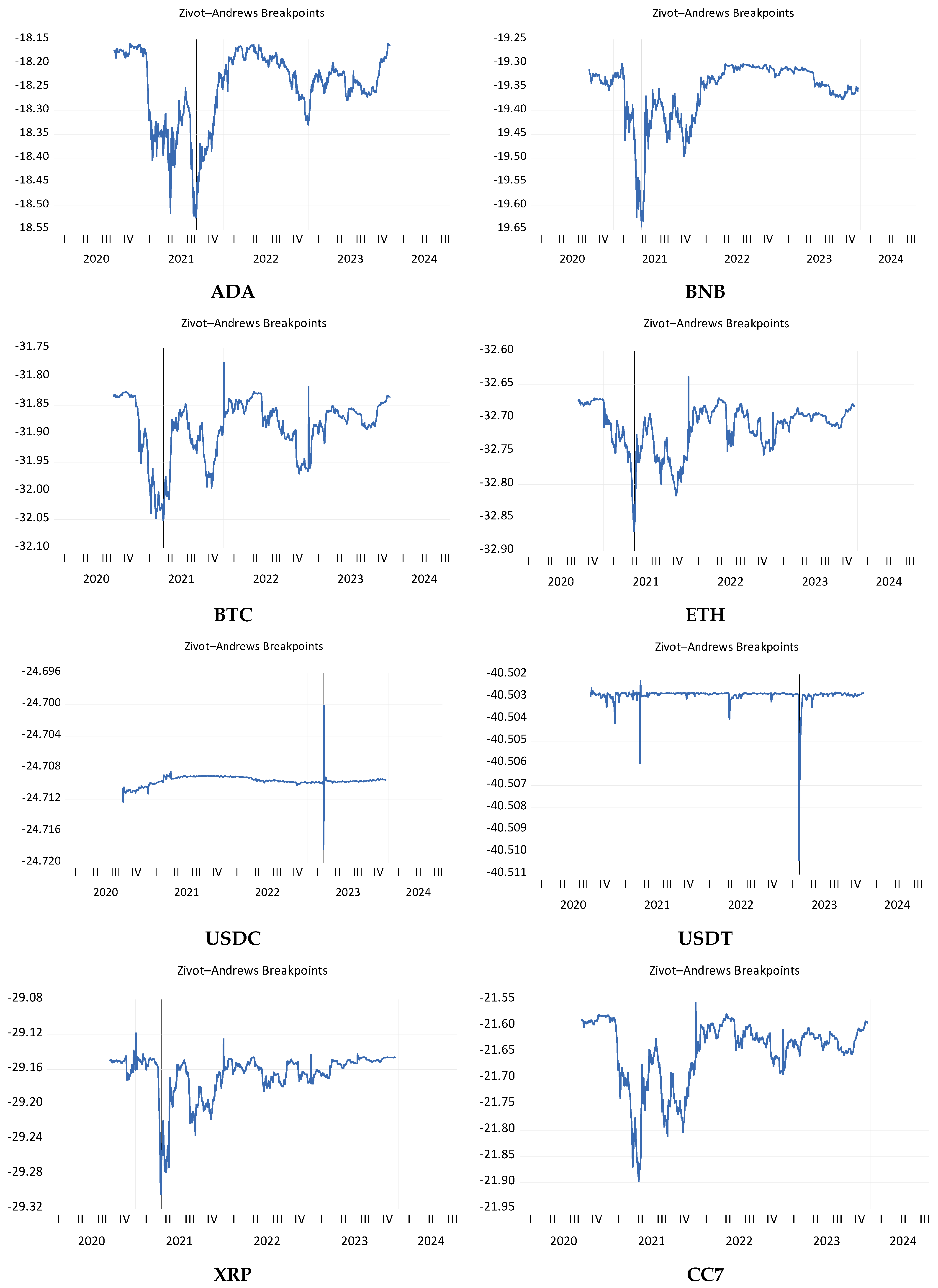
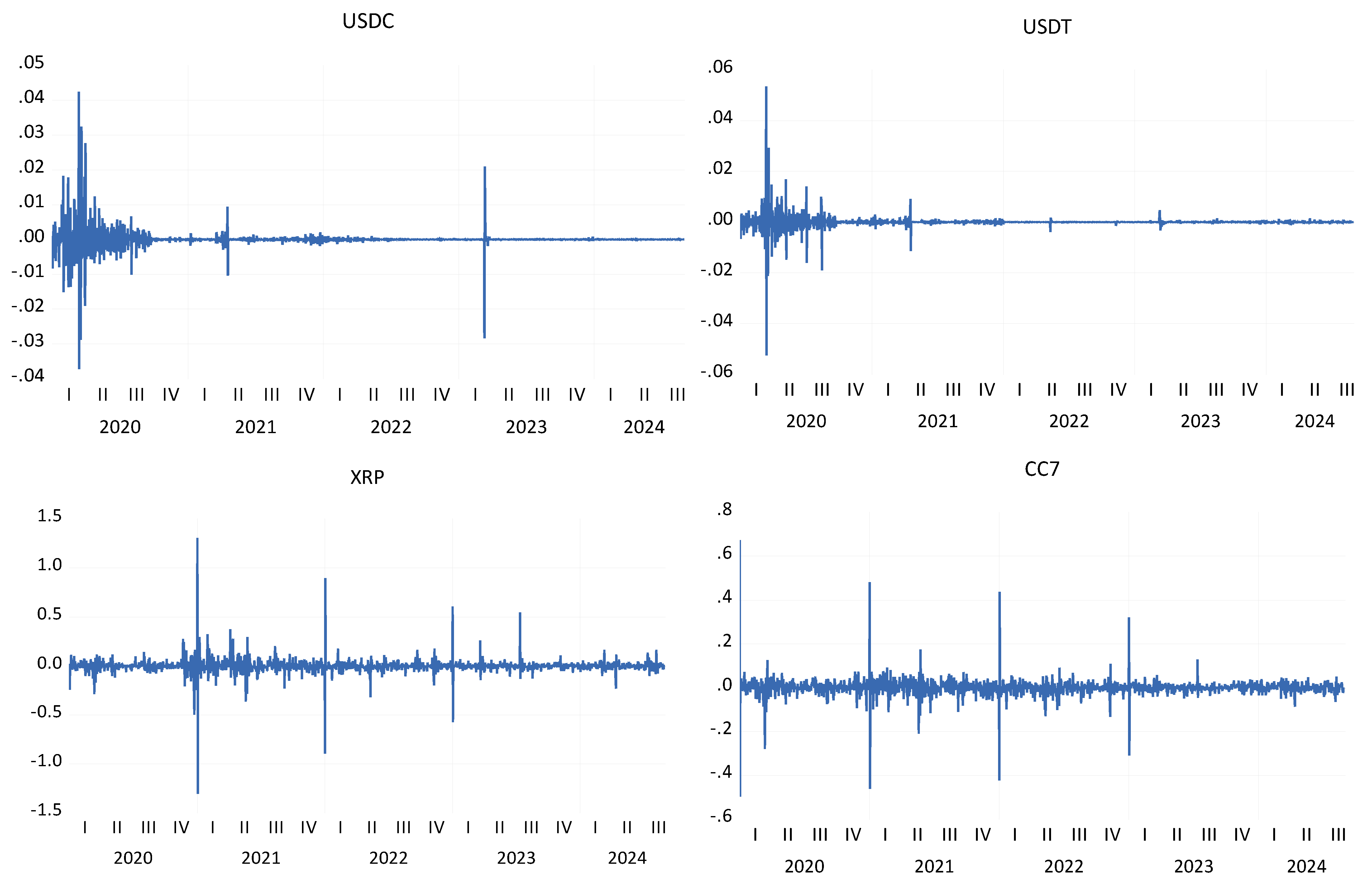
5.2. Stationarity Investigation

To assess the stability of returns, the Augmented Dickey–Fuller (ADF) test was conducted. The outcomes of the ADF test are summarized in

Table 6. The outcomes of ADF test.

	ADA	BNB	BTC	ETH	USDC	USDT	XRP	CC7
t-Statistic	−44.29567	−28.6233	−31.839	−32.637	−16.9532	−18.2710	−29.1545	−62.3745
Prob	0.0001	0.0000	0.0000	0.0000	0.0000	0.0000	0.00000	0.0001
Lag Length Schwarz info criterion	0	1	2	2	10	18	2	0
AIC	−3.0860	−3.2551	−2.9027	−2.3062	−9.3204	0.96476	−2.3089	−3.7837
F-statistic Prob (F-statistic)	1962.106 0.000000	1020.889 0.000000	1221.906 0.000000	1288 0.000000	467.650 0.000000	389.813 0.000000	1013.220 0.000000	3890.588 0.000000
Test critical values
1%			−3.433984
5%			−2.863032
10%			−2.567612

which demonstrates that for all cryptocurrencies and the CC7 index, the test statistics are significantly lower than the 1% critical value (−3.4339), leading to the rejection of the null hypothesis (H₀) of a unit root. Thus, all return series are stationary, indicating mean-reverting behavior with no unit root presence. Stablecoins USDC and USDT required higher lag lengths (10 and 18, respectively), reflecting their unique price stabilization mechanisms.

The Zivot–Andrews unit root test further validates stationarity by accounting for potential structural breaks.

Table 7. The outcomes of the Zivot–Andrews unit root test.

	ADA	BNB	BTC	ETH	USDC	USDT	XRP	CC7
t-Statistic	−18.52625	−19.64573	−32.05270	−32.87102	−24.71840	−40.51040	−29.30377	−21.89878
Prob	0.000217	0.000104	0.000320	0.001111	0.008155	0.067926	0.005545	0.000116
Chosen lag length	4	3	2	2	4	2	2	3
Chosen break point	4 September 2021	4 May 2021	16 April 2021	13 May 2021	13 March 2023	13 March 2023	16 April 2021	10 May 2021
Critical Values
1%			−5.34
5%			−4.93
10%			−4.58

shows that the null hypothesis of a unit root with a structural break in the intercept is rejected across all assets, confirming stationarity. The identified breakpoints suggest market-wide structural shifts, with BTC and XRP experiencing breaks on 16 April 2021, possibly linked to the mid-2021 crypto bull market peak. Similarly, BNB, ETH, and CC7 display breakpoints in May 2021, coinciding with the market downturn following China’s crypto crackdown and regulatory tightening. USDC and USDT share a breakpoint on 13 March 2023, which may correspond to financial stability concerns or macroeconomic events affecting stablecoin usage.

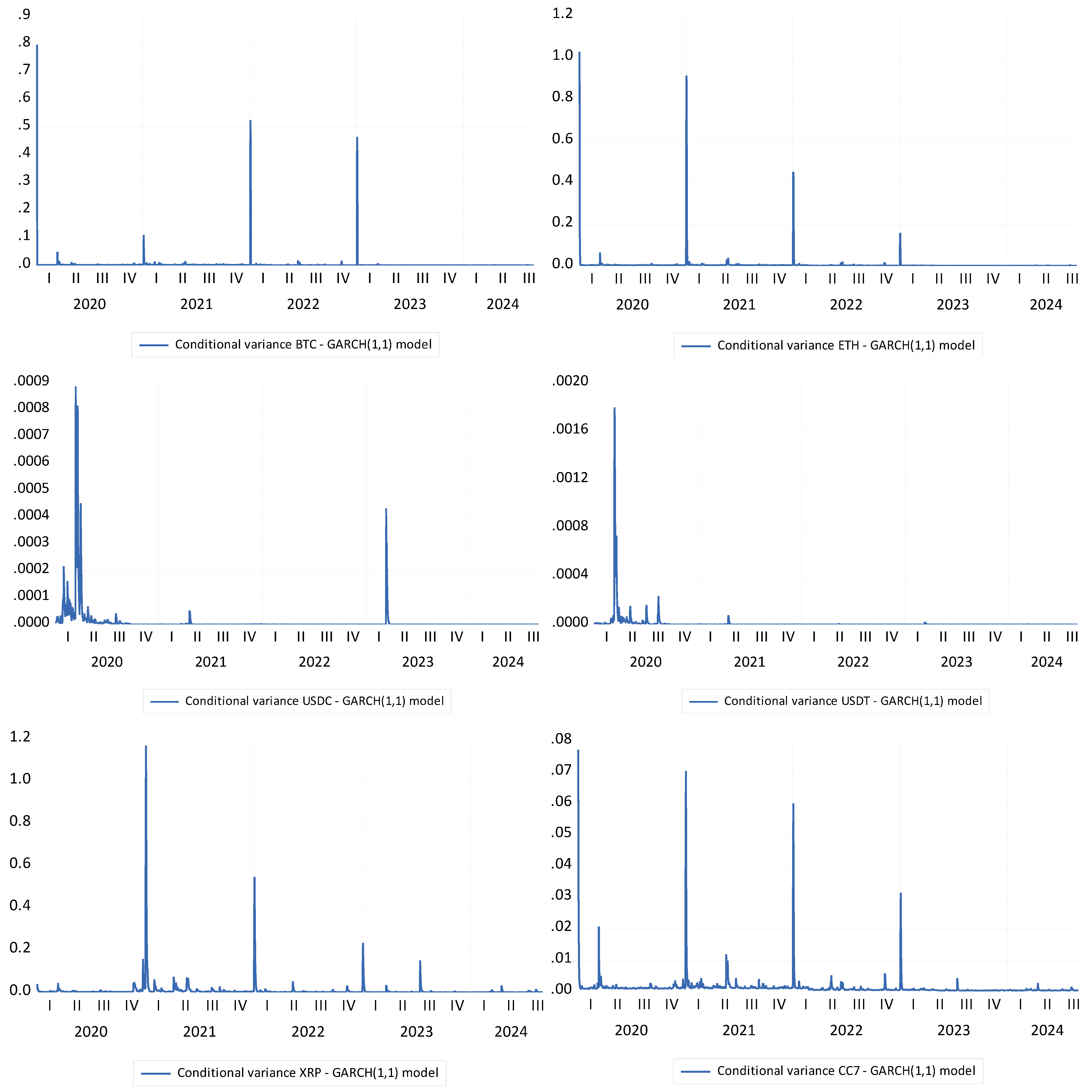
5.3. Outcomes of GARCH(1,1) Model

The GARCH(1,1) model results provide valuable insights into the volatility dynamics of various cryptocurrencies, including ADA, BNB, BTC, ETH, USDC, USDT, XRP, and the crypto index CC7. The model consists of two main components: the mean equation, which captures the return-generating process, and the variance equation, which models the persistence of volatility. Additionally, exogenous variables such as COVID-19 and geopolitical events are included to examine their effects on market fluctuations.

The mean equation results in

Table 8. GARCH(1,1) model estimation results for cryptocurrency volatility: impact of COVID-19 and the Russia–Ukraine war.

	ADA	BNB	BTC	ETH	USDC	USDT	XRP	CC7
Mean Equation
C	−0.0004	0.0012	0.0011	0.0018	0.0000	0.0000	−0.0003	0.0016
Prob	0.6254	0.0533	0.0531	0.0090	0.8817	0.6402	0.6323	0.0006
Dependent Variable(−1)	−0.0715	−0.0832	−0.0775	−0.0666	−0.4143	−0.3134	−0.1079	−0.0681
Prob	0.0037	0.0000	0.0009	0.0058	0.0000	0.0000	0.0000	0.0058
Variance Equation
C	0.0004	0.0003	0.0020	0.0021	0.0000	0.0000	0.0009	0.0004
Prob	0.0006	0.0006	0.0004	0.0000	0.0001	0.0001	0.0023	0.0000
RESID(−1)^2	0.1839	0.1866	0.4948	0.3530	0.5287	0.6089	0.5013	0.2453
Prob	0.0000	0.0000	0.0024	0.0002	0.0000	0.0000	0.0008	0.0000
GARCH(−1)	0.7319	0.7577	−0.0050	0.1386	0.5890	0.5998	0.5566	0.4259
Prob	0.0000	0.0000	0.3247	0.0428	0.0000	0.0000	0.0000	0.0000
COVID-19	0.0001	0.0000	0.0004	0.0008	0.0000	0.0000	0.0002	0.0001
Prob	0.2021	0.0922	0.0289	0.0003	0.5874	0.0008	0.1667	0.0170
WAR	−0.0002	−0.0002	−0.0011	−0.0015	0.0000	0.0000	−0.0005	−0.0003
Prob	0.0046	0.0022	0.0028	0.0001	0.0005	0.0047	0.0203	0.0001
T-DIST. DOF	4.0505	3.3443	2.5064	2.7636	3.4263	3.0047	2.4873	3.2213
Prob	0.0000	0.0000	0.0000	0.0000	0.0000	0.0000	0.0000	0.0000
Information Criteria
Akaike info criterion	−3.4190	−3.8963	−4.1350	−3.6800	−13.0358	−12.5976	−3.5886	−4.6334
Schwarz criterion	−3.3934	−3.8708	−4.1095	−3.6544	−13.0102	−12.5720	−3.5631	−4.6078
Hannan–Quinn criterion	−3.4095	−3.8868	−4.1256	−3.6705	−13.0263	−12.5881	−3.5792	−4.6239
Residual Diagnostics
Correlogram of Standardized Residuals
AC(5)	−0.013	0.002	−0.017	0.016	−0.0020	−0.003	−0.009	0.01
PAC(5)	−0.018	−0.005	−0.018	0.017	−0.0020	−0.005	−0.01	0.011
Q-Stat(5)	10.274	14.382	6.5463	6.2781	5.6698	7.2255	2.2811	6.0096
Prob	0.068	0.013	0.257	0.28	0.3400	0.204	0.809	0.305
AC(10)	0.018	0.017	−0.006	−0.026	−0.0140	−0.024	−0.004	0.002
PAC(10)	0.016	0.017	−0.007	−0.029	−0.0140	−0.025	−0.004	0.001
Q-Stat(10)	22.216	18.842	8.4463	10.454	6.1290	10.497	3.9181	7.3358
Prob	0.014	0.042	0.585	0.402	0.8040	0.398	0.951	0.693
AC(20)	0.004	−0.037	−0.02	0.005	0.0070	−0.003	−0.006	0.007
PAC(20)	−0.003	−0.038	−0.017	0.005	0.0070	−0.006	−0.008	0.01
Q-Stat(20)	30.328	27.208	14.685	14.551	9.0969	16.768	6.8351	14.306
Prob	0.065	0.13	0.794	0.801	0.9820	0.668	0.997	0.815
Correlogram of Standardized Residuals Squared
AC(5)	0.0060	0.0070	−0.0020	−0.0020	−0.0010	−0.0030	−0.0070	−0.0060
PAC(5)	0.0060	0.0080	−0.0020	−0.0020	−0.0010	−0.0030	−0.0070	−0.0060
Q-Stat(5)	2.8133	6.3805	0.0371	0.0426	0.0051	0.0422	0.2163	0.3614
Prob	0.7290	0.2710	1.0000	1.0000	1.0000	1.0000	0.9990	0.9960
AC(10)	−0.0050	−0.0120	−0.0020	0.0110	−0.0010	−0.0030	0.0020	0.0050
PAC(10)	−0.0050	−0.0100	−0.0020	0.0110	−0.0010	−0.0030	0.0020	0.0050
Q-Stat(10)	4.7305	7.5681	0.0926	0.2864	0.0106	0.0998	0.3348	0.7488
Prob	0.9080	0.6710	1.0000	1.0000	1.0000	1.0000	1.0000	1.0000
AC(20)	−0.0130	−0.0210	0.0020	0.0030	−0.0010	−0.0030	0.0060	0.0120
PAC(20)	−0.0160	−0.0220	0.0010	0.0030	−0.0010	−0.0030	0.0060	0.0110
Q-Stat(20)	11.8160	11.2410	0.1679	0.3937	0.0202	0.1778	0.7526	1.3534
Prob	0.9220	0.9400	1.0000	1.0000	1.0000	1.0000	1.0000	1.0000

indicate that most cryptocurrencies exhibit statistically insignificant mean returns, implying that their price movements are largely unpredictable. However, ETH shows a significant positive return (0.0018, p = 0.0090), suggesting a momentum effect. BNB and BTC exhibit marginally significant positive returns (p = 0.0533 and p = 0.0531, respectively), suggesting at some predictability. Additionally, stablecoins (USDC and USDT) have near-zero returns, aligning with their pegged nature. The lagged dependent variable reveals a negative and significant effect across all cryptocurrencies, indicating mean reversion. For instance, BTC (−0.0775, p = 0.0009) and ETH (−0.0666, p = 0.0058) show moderate mean reversion. Stablecoins USDC (−0.3134, p = 0.0000) and USDT (−0.4143, p = 0.0000) exhibit stronger mean reversion patterns.

The variance equation confirms high volatility persistence across all assets. The RESID(−1)^2 term, capturing past shocks, is significant for all cryptocurrencies, emphasizing the role of past volatility in future price fluctuations. The GARCH(−1) term, which measures long-term volatility persistence, is close to or above 0.5 for most assets. COVID-19 significantly increased volatility for BTC (0.0004, p = 0.0289), ETH (0.0008, p = 0.0003), USDC (0.0000, p = 0.0008), and CC7 (0.0001, p = 0.0170). In contrast, the war variable shows a negative effect on volatility for BTC (−0.0011, p = 0.0028), ETH (−0.0015, p = 0.0001), and XRP (−0.0005, p = 0.0203). This suggests that investors adjusted their risk exposure, reducing speculative activity during geopolitical instability.

A fundamental observation in

Table 9. Volatility dynamics: combined ARCH and GARCH term estimates in GARCH(1,1) model.

ARCH + GARCH Terms	ADA	BNB	BTC	ETH	USDC	USDT	XRP	CC7
RESID(−1)^2 + GARCH (−1)	0.9158	0.9443	0.4898	0.4916	1.1177	1.2087	1.0579	0.6712

is the sum of the ARCH (RESID(−1)^2) and GARCH(−1) terms, which determines volatility persistence. For instance, for BTC, ETH, and CC7, the sum is below 1, indicating mean-reverting volatility where shocks dissipate over time. However, for USDC, USDT, and XRP, the sum exceeds 1, implying high persistence or potential non-stationarity—unexpected for stablecoins, which are designed to maintain low volatility.

Table 10. Testing for ARCH effects in GARCH(1,1) model: LM test results.

ARCH LM Test (Lag = 1)	ADA	BNB	BTC	ETH	USDC	USDT	XRP	CC7
F-statistic	0.3611	0.2443	0.0002	0.0003	0.0009	0.0000	0.0072	0.0389
Prob(F-statistic)	0.5480	0.6212	0.9897	0.9863	0.9767	0.9999	0.9323	0.8437
Obs*R-squared	0.3614	0.2446	0.0002	0.0003	0.0009	0.0000	0.0072	0.0389
Prob. Chi-Square	0.5477	0.6209	0.9897	0.9863	0.9767	0.9999	0.9322	0.8436

further confirms the adequacy of the GARCH(1,1) model through the ARCH-LM test, where all p-values exceed 0.05, indicating that the model effectively captures volatility clustering.

Figure 2 illustrates the conditional variance (CV) of log returns for the analyzed cryptocurrencies. ADA and BNB exhibited higher volatility than BTC during the study period. ADA’s peak volatility occurred on 13 March 2020, while BNB’s highest volatility was observed on 20 February 2021.

The results from the GARCH(1,1) model provide strong evidence for the following confirmed and partially confirmed hypotheses:

• H1.2 (volatility persistence during financial crises) is confirmed. The persistence of volatility, particularly during periods of crisis like COVID-19, is evident from the significant ARCH and GARCH coefficients across major cryptocurrencies (BTC, ETH, USDC, and CC7). This persistence indicates that shocks from these crises had a lasting effect on market volatility, which is consistent with the existing literature on volatility clustering during turbulent periods.
• H2.2 (amplified volatility during negative price shocks) is partially confirmed. While cryptocurrencies like BTC and ETH exhibited significant volatility increases during negative price shocks such as COVID-19, this effect was not uniform across all assets. For instance, stablecoins such as USDC and USDT showed minimal or no amplification, which suggests that, while negative shocks can heighten volatility for many digital assets, their impact may vary depending on the asset type and market dynamics.
• H3.2 (COVID-19’s stronger impact on volatility compared to the Russia–Ukraine war) is confirmed. The COVID-19 pandemic had a more widespread and pronounced effect on cryptocurrency volatility compared to the Russia–Ukraine war. Significant increases in volatility for assets like BTC, ETH, and USDC during the pandemic highlight the global economic shockwaves it generated, in contrast to the more localized impact of geopolitical instability from the war, which showed negative correlations with volatility in certain assets.
• H4.2 (stablecoins as risk-hedging instruments) is partially confirmed. While stablecoins such as USDC and USDT exhibited relative stability during the COVID-19 crisis, their role as effective risk-hedging instruments was somewhat limited. This limitation stems from issues like liquidity concerns and the reliance on traditional financial systems that could restrict their utility in extreme market conditions. Despite their relatively stable prices, stablecoins may not offer the full protection expected from traditional safe-haven assets.

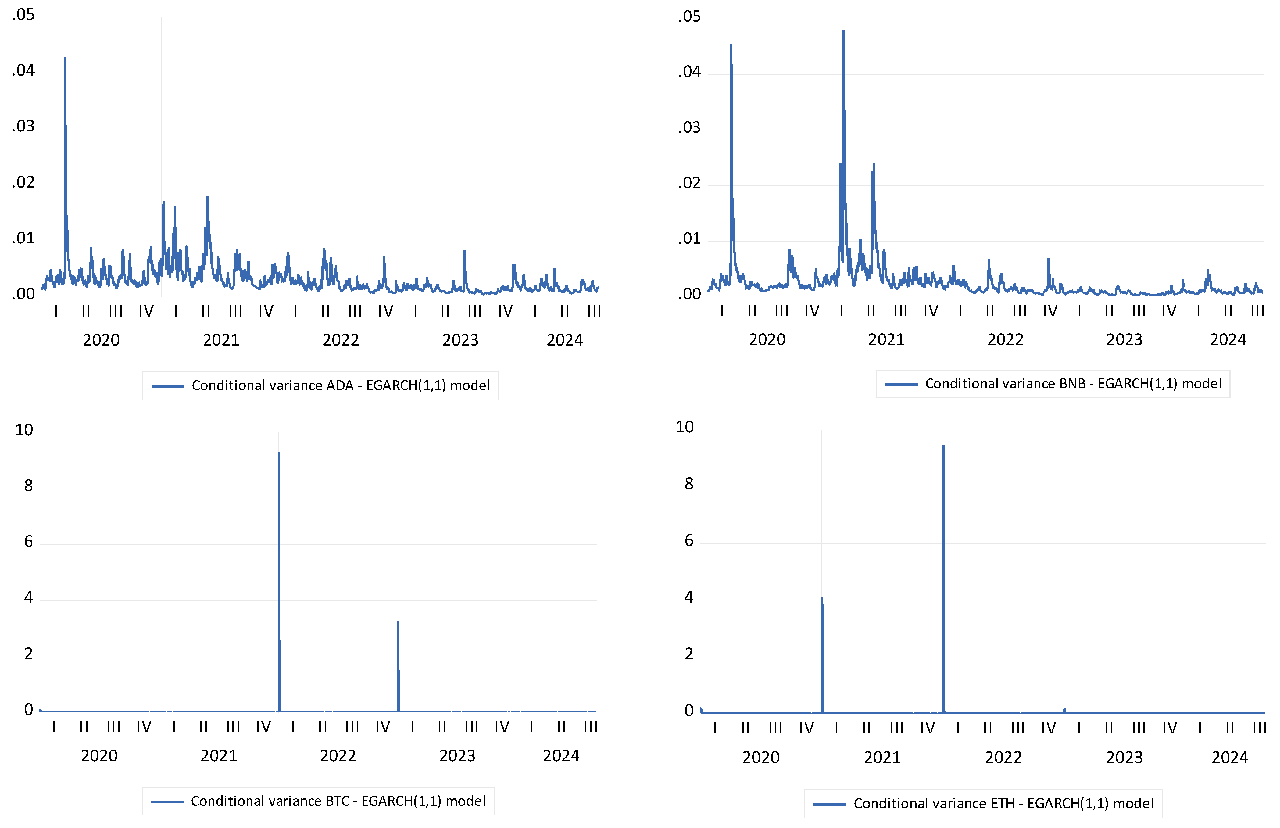
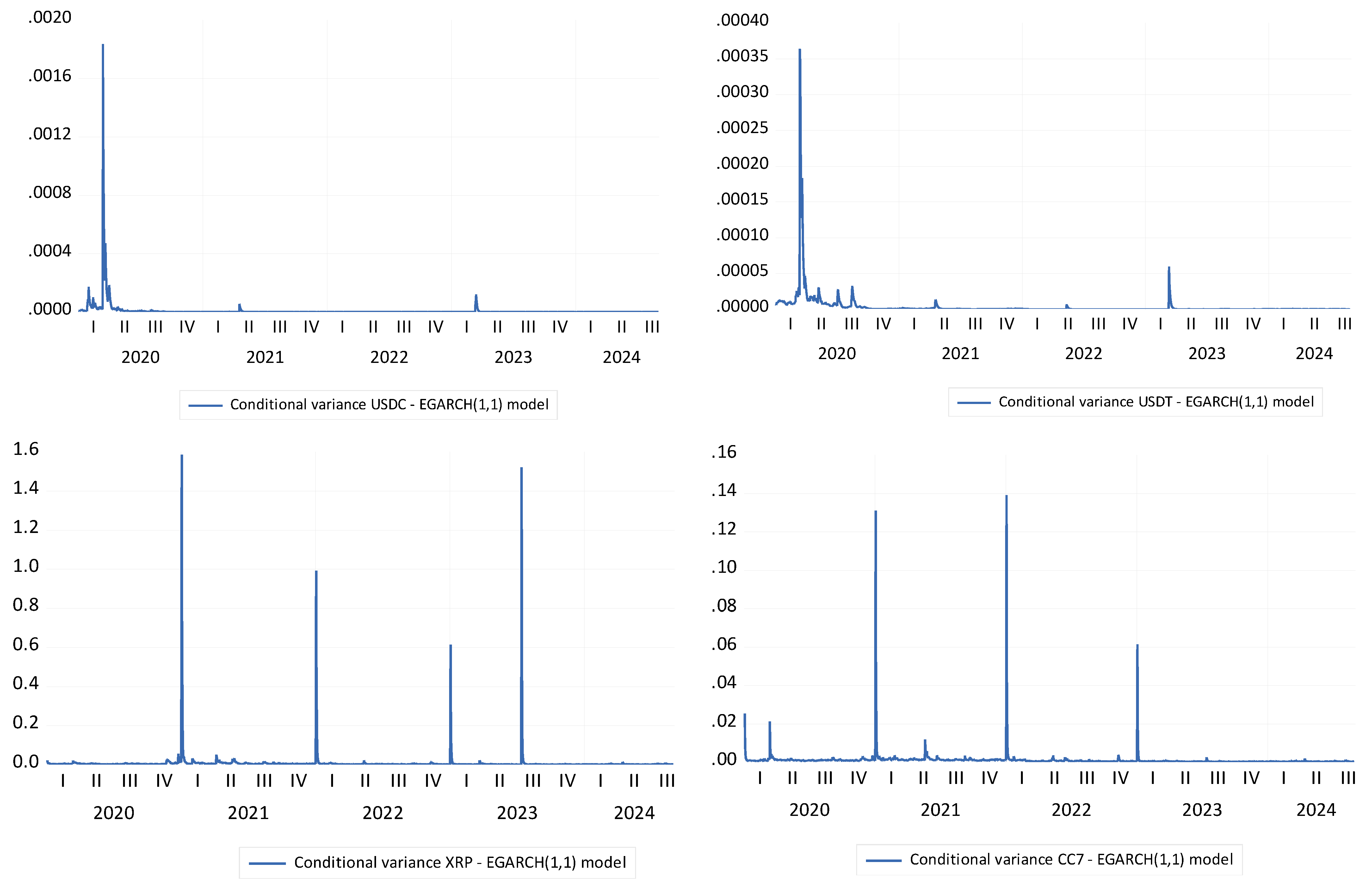
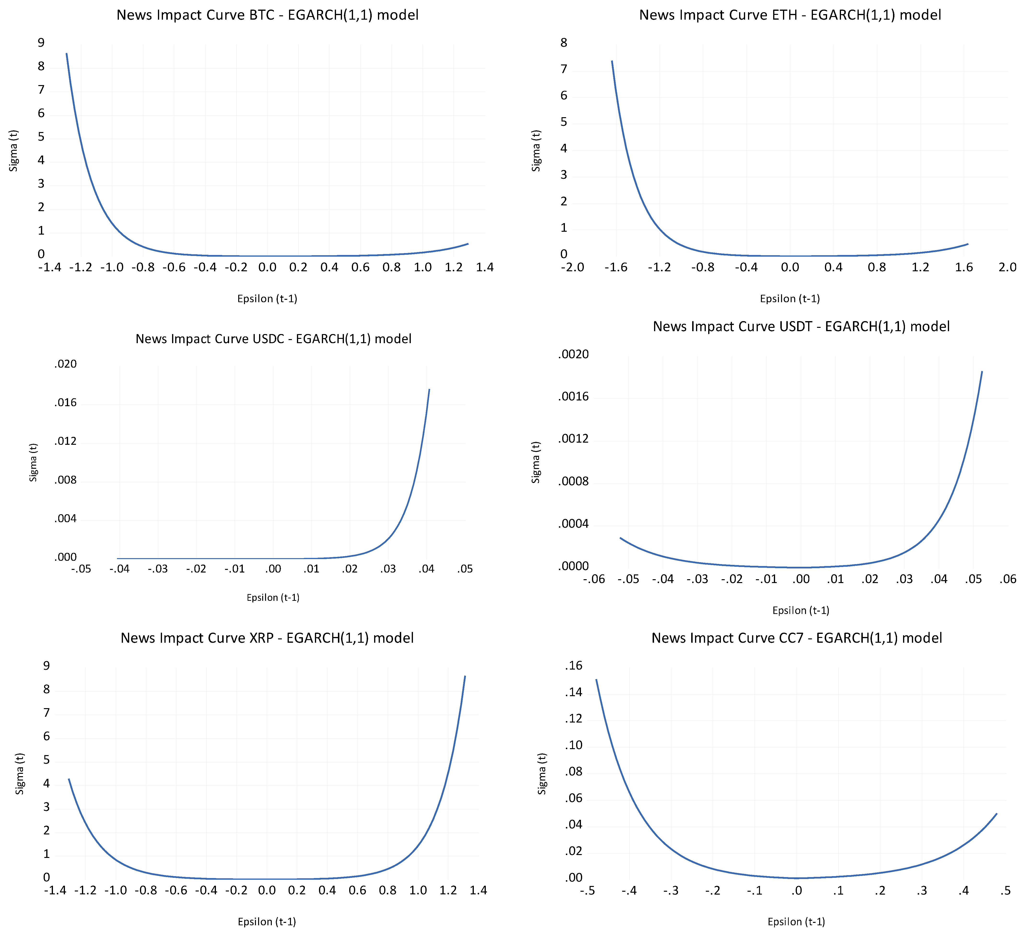
5.4. Outcomes of EGARCH(1,1) Model

The outcomes of the EGARCH(1,1) model are provided in

Table 11. Volatility dynamics in cryptocurrencies: EGARCH(1,1) analysis of COVID-19 and the Russia–Ukraine war.

	ADA	BNB	BTC	ETH	USDC	USDT	XRP	CC7
Mean Equation
C	−0.0003	0.0013	0.0009	0.0016	0.0000	0.0000	−0.0003	0.0014
Prob	0.7293	0.0405	0.1192	0.0233	0.3812	0.5618	0.7071	0.0032
Dependent Var(−1)	−0.0748	−0.0829	−0.0668	−0.0523	−0.4092	−0.3089	−0.0990	−0.0582
Prob	0.0020	0.0000	0.0017	0.0221	0.0000	0.0000	0.0000	0.0166
Variance Equation
C(3)	−0.8512	−0.6691	−2.4537	−1.8860	−0.5414	−0.5348	−1.1759	−2.0915
Prob	0.0000	0.0000	0.0000	0.0000	0.0000	0.0000	0.0000	0.0000
C(4)	0.3290	0.3207	0.3453	0.3322	0.2771	0.2265	0.4288	0.3538
Prob	0.0000	0.0000	0.0000	0.0000	0.0000	0.0000	0.0000	0.0000
C(5)	0.0110	0.0139	−0.0725	−0.0765	0.2360	0.0425	0.0209	−0.0439
Prob	0.6880	0.5907	0.1068	0.0235	0.0000	0.0137	0.5415	0.1901
C(6)	0.8946	0.9247	0.6304	0.7249	0.9727	0.9657	0.8284	0.7361
Prob	0.0000	0.0000	0.0000	0.0000	0.0000	0.0000	0.0000	0.0000
C(7)	0.0271	0.0198	0.1183	0.1764	−0.0404	−0.0962	0.0421	0.0999
Prob	0.2978	0.3542	0.0450	0.0008	0.0043	0.0000	0.2360	0.0331
C(8)	−0.0847	−0.0842	−0.2363	−0.2100	−0.1018	−0.1248	−0.1208	−0.2158
Prob	0.0047	0.0025	0.0005	0.0002	0.0000	0.0000	0.0023	0.0002
T-DIST. DOF	4.1216	3.3678	2.5132	2.8338	3.2478	2.9373	2.5043	3.2895
Prob	0.0000	0.0000	0.0000	0.0000	0.0000	0.0000	0.0000	0.0000
Information Criteria
Akaike info criterion	−3.4196	−3.8921	−4.1333	−3.6885	−12.9972	−12.5621	−3.5874	−4.6381
Schwarz criterion	−3.3908	−3.8634	−4.1046	−3.6598	−12.9684	−12.5334	−3.5586	−4.6094
Hannan–Quinn criterion	−3.4089	−3.8815	−4.1227	−3.6778	−12.9865	−12.5515	−3.5767	−4.6275
Residual Diagnostics
Correlogram of Standardized Residuals
AC(5)	−0.014	0.005	0.001	0.008	0.0010	−0.007	−0.009	−0.013
PAC(5)	−0.019	−0.003	0.001	0.008	0.0010	−0.01	−0.011	−0.014
Q-Stat(5)	10.919	15.656	3.0811	4.2577	0.6970	10.045	3.0769	6.001
Prob	0.053	0.008	0.687	0.513	0.9830	0.074	0.688	0.306
AC(10)	0.016	0.016	0.000	−0.021	−0.0080	−0.023	−0.013	−0.007
PAC(10)	0.014	0.016	−0.001	−0.023	−0.0080	−0.023	−0.013	−0.008
Q-Stat(10)	23.133	19.777	3.9312	7.1781	0.8668	13.677	6.775	8.0002
Prob	0.01	0.031	0.95	0.709	1.0000	0.188	0.747	0.629
AC(20)	0.006	−0.034	0.01	0.008	0.0020	0.001	−0.01	−0.019
PAC(20)	−0.001	−0.036	0.012	0.008	0.0020	−0.003	−0.014	−0.017
Q-Stat(20)	31.756	27.871	11.489	10.627	1.6696	18.876	9.3528	14.028
Prob	0.046	0.112	0.933	0.955	1.0000	0.53	0.978	0.829
Correlogram of Standardized Residuals Squared
AC(5)	0.0070	0.0070	−0.0020	−0.0020	−0.0010	−0.0030	−0.0070	−0.0050
PAC(5)	0.0070	0.0080	−0.0020	−0.0020	−0.0010	−0.0030	−0.0070	−0.0050
Q-Stat(5)	2.7261	5.8385	0.0415	0.0620	0.0027	0.0413	0.2045	0.2582
Prob	0.7420	0.3220	1.0000	1.0000	1.0000	1.0000	0.9990	0.9980
AC(10)	−0.0030	−0.0090	−0.0020	0.0060	−0.0010	−0.0030	0.0050	0.0020
PAC(10)	−0.0030	−0.0070	−0.0020	0.0060	−0.0010	−0.0030	0.0050	0.0020
Q-Stat(10)	5.0459	7.1726	0.0891	0.1769	0.0059	0.0964	0.4031	0.4993
Prob	0.8880	0.7090	1.0000	1.0000	1.0000	1.0000	1.0000	1.0000
AC(20)	−0.0130	−0.0200	0.0010	0.0020	−0.0010	−0.0030	0.0040	0.0080
PAC(20)	−0.0150	−0.0220	0.0010	0.0020	−0.0010	−0.0030	0.0040	0.0080
Q-Stat(20)	12.0220	10.7310	0.1454	0.2663	0.0120	0.1913	0.8413	0.9213
Prob	0.9150	0.9530	1.0000	1.0000	1.0000	1.0000	1.0000	1.0000

. With reference to the mean equation, BNB, ETH, and CC7 showed statistically significant positive intercepts, indicating that these assets experienced positive returns significantly different from zero during the sample period. This suggests that, on average, these cryptocurrencies exhibited upward growth trends. ADA, XRP, and USDC did not show significant intercepts, implying that their returns did not exhibit consistent, predictable trends and were likely driven by market fluctuations rather than long-term growth.

The negative and significant coefficients for the lagged dependent variable (e.g., Dependent Var(−1)) for most cryptocurrencies signal mean-reverting behavior. This means that positive returns in one period are typically followed by negative returns in the subsequent period, indicative of short-term corrections and volatility in cryptocurrency markets. The strongest negative coefficients were found for ADA, BNB, and BTC, suggesting these cryptocurrencies exhibit a particularly high sensitivity to prior market movements.

As regards the variance equation, relating to the leverage effect (C(3)), all cryptocurrencies exhibited negative and significant leverage coefficients, indicating that negative shocks (such as price drops) lead to higher volatility compared to positive shocks of equal magnitude. This behavior is a fundamental characteristic of asymmetric volatility, where bad news has a more significant impact than good news. Volatility persistence (C(4) and C(6)) provides support for positive and significant coefficients for past volatility innovations, and the high values of the volatility persistence coefficient indicate that volatility shocks tend to persist over time. This outcome is consistent with the notion of volatility clustering, where periods of high volatility tend to be followed by more high volatility and periods of low volatility by continued low volatility. Decay in volatility (C(8)) emphasized by the negative and significant coefficient suggests that volatility tends to decrease over time, as markets adapt to and stabilize after initial shocks. However, this process is gradual, as evidenced by the high persistence of volatility in many cryptocurrencies.

The correlogram of standardized residuals shows that the EGARCH(1,1) model adequately captures the temporal dependencies in the data, as evidenced by the insignificant autocorrelation and partial autocorrelation values and no significant autocorrelation in the residuals (Q-statistics).

The ARCH LM test results reported in

Table 12. Evaluation of heteroskedasticity: ARCH LM test on EGARCH(1,1) model.

ARCH LM Test (Lag = 1)	ADA	BNB	BTC	ETH	USDC	USDT	XRP	CC7
F-statistic	0.1988	0.0406	0.0065	0.0088	0.0002	0.0015	0.0212	0.0142
Prob(F-statistic)	0.6557	0.8404	0.9358	0.9252	0.9889	0.9686	0.8844	0.9052
Obs*R-squared	0.1991	0.0406	0.0065	0.0088	0.0002	0.0015	0.0212	0.0142
Prob. Chi-Square	0.6555	0.8403	0.9358	0.9251	0.9889	0.9686	0.8843	0.9051

further support the reliability of the model, with all F-statistics and corresponding p-values greater than 0.05, indicating no remaining significant ARCH effects. This suggests that the EGARCH(1,1) model effectively captures the time-varying volatility structure.

The conditional variance analysis, as depicted in Figure 3, highlights significant volatility spikes during periods of market stress, such as March 2020 for ADA and February 2021 for BNB, confirming that major events (like the COVID-19 pandemic and significant market fluctuations) had a profound impact on volatility.

The news impact curves presented in Figure 4 reveal that negative news has a more significant impact on volatility than positive news, especially for BTC, ETH, and CC7. This reinforces the leverage effect and asymmetric volatility observed earlier, where negative shocks cause larger volatility spikes compared to positive developments.

The findings from the EGARCH(1,1) model offer compelling support for the hypotheses that are both fully and partially confirmed:

• The results support H1.2, showing significant positive coefficients for lagged volatility terms (C(4) and C(6)), indicating that volatility persists over time. High volatility tends to follow high volatility, especially during crises like the COVID-19 pandemic, confirming volatility clustering.
• H2.2 is confirmed by the negative and significant leverage effect (C(3)), which shows that negative shocks lead to higher volatility than positive shocks of equal magnitude. The news impact curves also reinforce this, highlighting that negative news has a stronger effect on volatility, especially for BTC, ETH, and CC7.
• The COVID-19 dummy (C(7)) has a stronger impact on volatility than the Russia–Ukraine war, supporting H3.2. The pandemic had a broader, more significant effect on market volatility, particularly for BTC and ETH, while the war’s impact was more localized.
• The results partially support H4.2. While USDC and USDT exhibit lower volatility than other cryptocurrencies; their lack of significant growth trends suggests they may not fully function as risk hedges, with liquidity being a limiting factor.

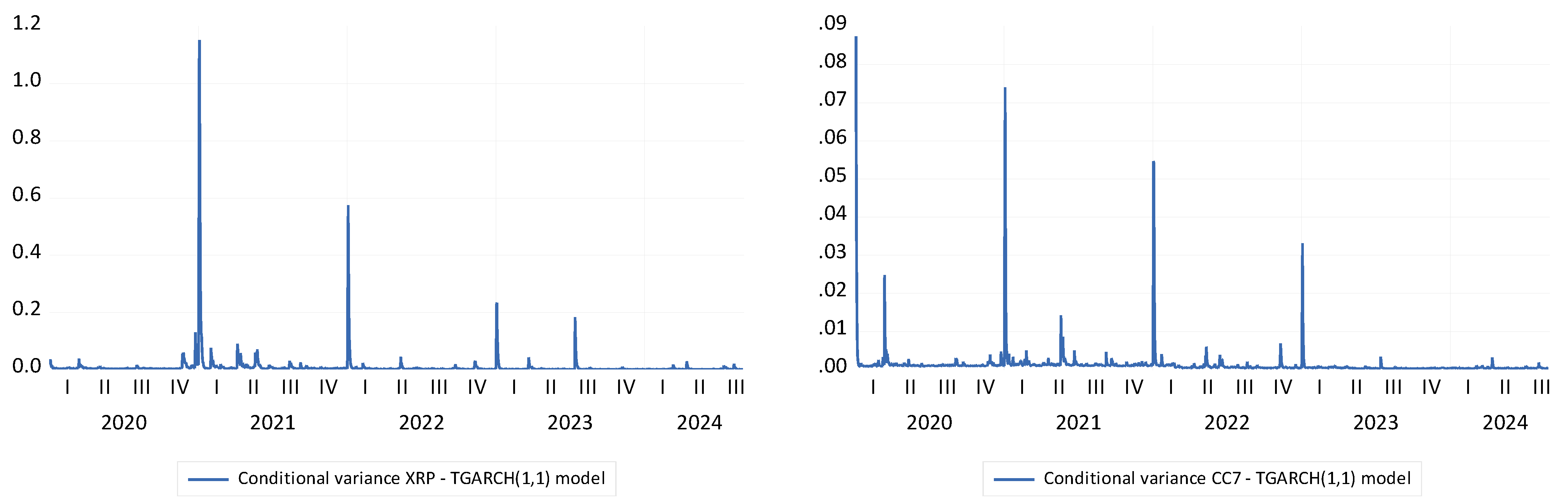
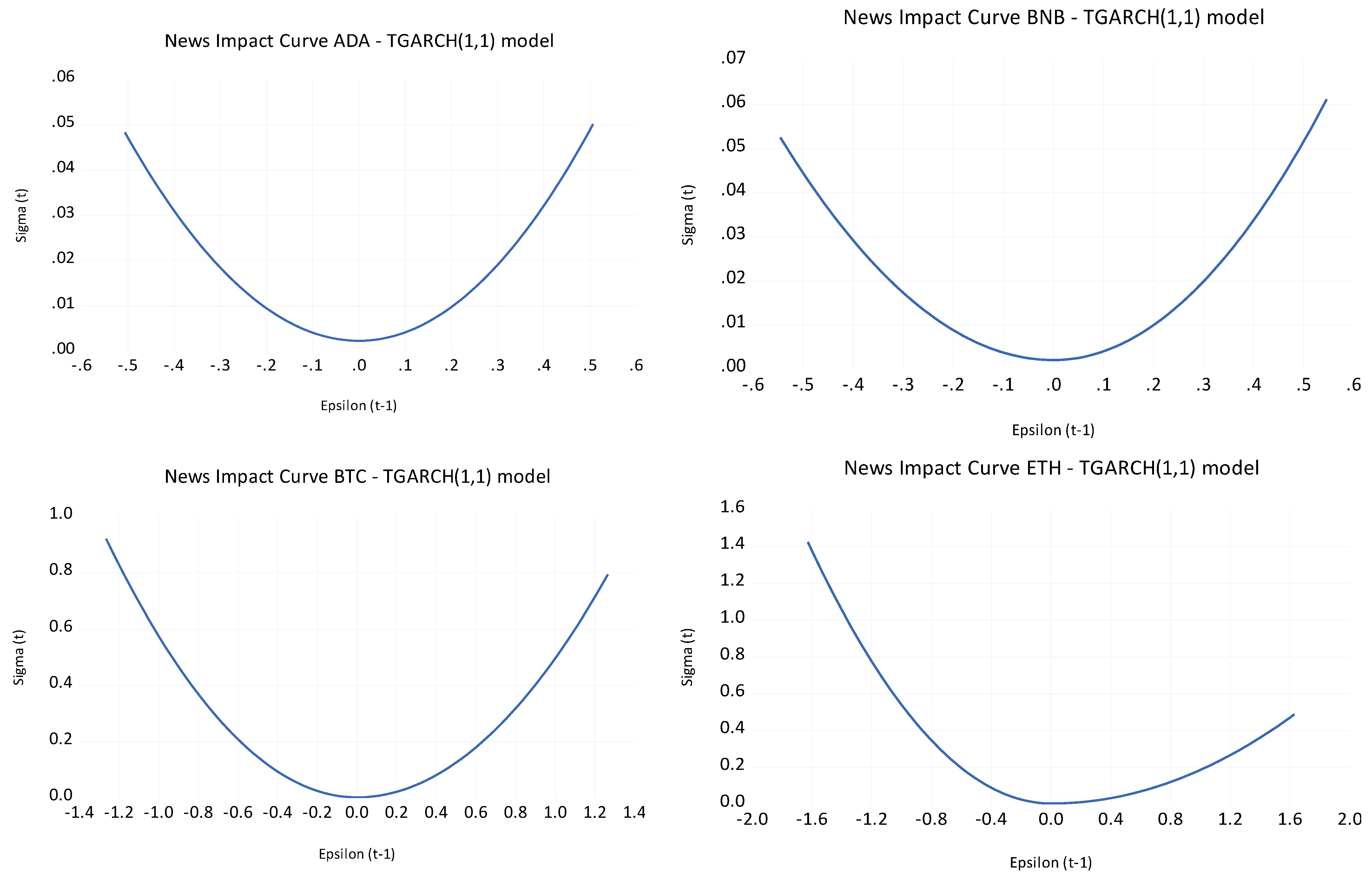
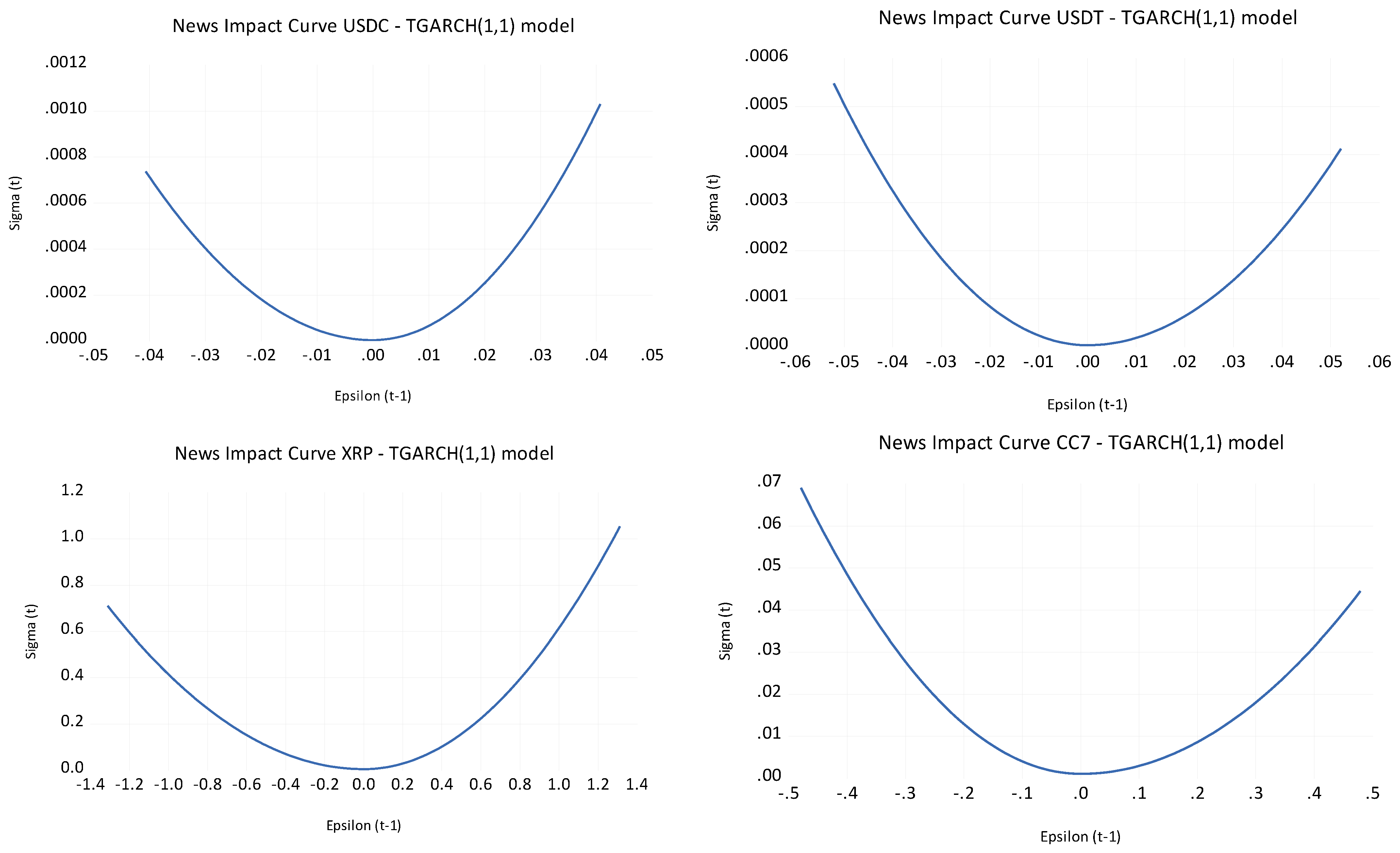
5.5. Outcomes of TGARCH(1,1) Model

Table 13. Impact of COVID-19 and the Russia–Ukraine war on cryptocurrency volatility: TGARCH(1,1) model results.

	ADA	BNB	BTC	ETH	USDC	USDT	XRP	CC7
Mean Equation
C	−0.0004	0.0013	0.0011	0.0016	0.0000	0.0000	−0.0002	0.0015
Prob	0.6410	0.0446	0.0546	0.0224	0.6664	0.5606	0.7895	0.0011
Dependent Variable(−1)	−0.0720	−0.0837	−0.0801	−0.0580	−0.4136	−0.4389	−0.1077	−0.0658
Prob	0.0034	0.0000	0.0006	0.0167	0.0000	0.0000	0.0000	0.0078
Variance Equation
C	0.0004	0.0003	0.0022	0.0020	0.0000	0.0000	0.0009	0.0005
Prob	0.0006	0.0007	0.0015	0.0000	0.0001	0.0000	0.0028	0.0000
RESID(−1)^2	0.1862	0.1987	0.4940	0.1828	0.6197	0.1503	0.6093	0.1893
Prob	0.0001	0.0001	0.0139	0.0149	0.0000	0.0000	0.0029	0.0077
RESID(−1)^2*(RESID(−1) < 0)	−0.0070	−0.0291	0.0793	0.3532	−0.1768	0.0501	−0.1997	0.1072
Prob	0.8894	0.5598	0.6988	0.0120	0.1962	0.0615	0.2127	0.2265
GARCH(−1)	0.7335	0.7627	−0.0051	0.1479	0.5903	0.5995	0.5603	0.4094
Prob	0.0000	0.0000	0.4252	0.0157	0.0000	0.0000	0.0000	0.0000
COVID-19	0.0001	0.0000	0.0004	0.0008	0.0000	0.0000	0.0002	0.0001
Prob	0.2017	0.0908	0.0383	0.0002	0.5904	0.0000	0.1667	0.0161
WAR	−0.0002	−0.0002	−0.0012	−0.0014	0.0000	0.0000	−0.0004	−0.0003
Prob	0.0047	0.0025	0.0054	0.0000	0.0005	0.0000	0.0244	0.0001
T-DIST. DOF	4.0497	3.3451	2.4586	2.8354	3.4151	20.0000	2.4775	3.2554
Prob	0.0000	0.0000	0.0000	0.0000	0.0000	0.0000	0.0000	0.0000
Information Criteria
Akaike info criterion	−3.4178	−3.8953	−4.1340	−3.6829	−13.0359	−12.2407	−3.5888	−4.6331
Schwarz criterion	−3.3891	−3.8666	−4.1052	−3.6542	−13.0071	−12.2120	−3.5600	−4.6044
Hannan–Quinn criterion	−3.4072	−3.8847	−4.1233	−3.6723	−13.0252	−12.2301	−3.5781	−4.6225
Residual Diagnostics
Correlogram of Standardized Residuals
AC(5)	−0.0140	0.0010	0.0100	0.0190	−0.0010	0.0000	−0.0110	−0.0160
PAC(5)	−0.0180	−0.0060	0.0110	0.0210	−0.0010	−0.0060	−0.0120	−0.0160
Q-Stat(5)	10.2900	14.3350	5.9341	6.7967	4.7094	25.7060	2.2776	6.3285
Prob	0.0670	0.0140	0.3130	0.2360	0.4520	0.0000	0.8100	0.2760
AC(10)	0.0170	0.0170	0.0020	−0.0270	−0.0130	−0.0480	−0.0040	−0.0050
PAC(10)	0.0160	0.0170	0.0010	−0.0290	−0.0130	−0.0500	−0.0040	−0.0060
Q-Stat(10)	22.2500	18.9560	7.2554	11.4880	5.1181	34.6120	4.0323	8.1580
Prob	0.0140	0.0410	0.7010	0.3210	0.8830	0.0000	0.9460	0.6130
AC(20)	0.0040	−0.0370	0.0070	0.0070	0.0070	0.0060	−0.0050	−0.0200
PAC(20)	−0.0030	−0.0390	0.0100	0.0070	0.0070	−0.0040	−0.0080	−0.0180
Q-Stat(20)	30.4320	27.2550	14.3940	15.7910	7.7829	48.6840	6.9948	14.4320
Prob	0.0630	0.1280	0.8100	0.7300	0.9930	0.0000	0.9970	0.8080
Correlogram of Standardized Residuals Squared
AC(5)	0.006	0.007	−0.002	−0.002	−0.0010	−0.003	−0.007	−0.006
PAC(5)	0.006	0.009	−0.002	−0.002	−0.0010	−0.003	−0.007	−0.006
Q-Stat(5)	2.795	6.738	0.037	0.058	0.0045	0.102	0.203	0.417
Prob	0.731	0.241	1.000	1.000	1.0000	1.000	0.999	0.995
AC(10)	−0.005	−0.013	−0.002	0.011	−0.0010	−0.002	0.002	0.005
PAC(10)	−0.006	−0.012	−0.002	0.011	−0.0010	−0.002	0.002	0.005
Q-Stat(10)	4.729	8.145	0.092	0.319	0.0096	0.181	0.325	0.788
Prob	0.909	0.615	1.000	1.000	1.0000	1.000	1.000	1.000
AC(20)	−0.013	−0.021	0.001	0.003	−0.0010	−0.003	0.007	0.011
PAC(20)	−0.016	−0.023	0.001	0.003	−0.0010	−0.003	0.006	0.011
Q-Stat(20)	11.816	11.562	0.166	0.421	0.0186	0.242	0.744	1.361
Prob	0.922	0.930	1.000	1.000	1.0000	1.000	1.000	1.000

exhibits the results of the TGARCH(1,1) model, which integrates external factors such as the COVID-19 pandemic and the geopolitical conflict (WAR). The mean equation indicates that most cryptocurrency returns are not significantly different from zero, except for BNB and ETH, where the constant term is statistically significant. The negative coefficients for the lagged dependent variable suggest some mean reversion, where past returns negatively impact future returns, which is typical in volatile financial markets.

In the variance equation, the ARCH term (RESID(−1)^2) is significant for all cryptocurrencies, showing that past squared residuals influence current volatility. The leverage effect term (RESID(−1)^2*(RESID(−1) < 0)) varies across selected assets. ETH demonstrates a significant asymmetry (p = 0.012), indicating that negative shocks lead to greater volatility than positive ones, a common trait in speculative assets. In contrast, BTC and XRP do not exhibit significant leverage effects, suggesting a more symmetric response to shocks. The GARCH term (GARCH(−1)) is significant for most cryptocurrencies except BTC, implying that past volatility strongly affects current volatility.

The COVID-19 variable is statistically significant for BTC and ETH, indicating that the pandemic had a measurable impact on their volatility. The WAR variable shows significant negative coefficients for most cryptocurrencies, suggesting that geopolitical tensions generally reduce volatility. This may be due to a flight to safer assets or increased risk aversion, although the effect is less pronounced for USDC and USDT. The residual diagnostics confirm no significant autocorrelation, supporting the model’s adequacy.

Table 14. ARCH LM test diagnostics for TGARCH(1,1) model residuals.

ARCH LM Test (Lag = 1)	ADA	BNB	BTC	ETH	USDC	USDT	XRP	CC7
F-statistic	0.3478	0.2227	0.0001	0.0122	0.0006	0.0609	0.0050	0.0801
Prob(F-statistic)	0.5554	0.6370	0.9913	0.9122	0.9804	0.8051	0.9436	0.7772
Obs*R-squared	0.3481	0.2230	0.0001	0.0122	0.0006	0.0610	0.0050	0.0802
Prob. Chi-Square	0.5552	0.6368	0.9913	0.9121	0.9804	0.8050	0.9436	0.7771

presents the results of the ARCH LM test for the TGARCH(1,1) model, which further evaluates the model’s ability to capture volatility clustering. The test examines whether any significant ARCH effects remain in the residuals after fitting the model. The F-statistics and Prob(F-statistics) indicate that all p-values are greater than 0.05 for each cryptocurrency and the crypto index (CC7), suggesting that there are no significant remaining ARCH effects. The Obs*R-squared and Prob. Chi-Square values also show high p-values (all greater than 0.05), which further confirms that no significant ARCH effects remain in the residuals. These results suggest that the TGARCH(1,1) model effectively captures the volatility clustering phenomenon in the analyzed cryptocurrencies, with no significant autocorrelation in the squared residuals, validating its robustness for modeling volatility dynamics in these assets.

The TGARCH(1,1) model captures asymmetric volatility responses, with more pronounced leverage effects for speculative assets like BTC, ETH, and the crypto index (CC7). These assets show heightened sensitivity to negative shocks, supporting behavioral finance theories that suggest negative news events tend to trigger stronger market reactions. Conversely, stablecoins such as USDC and USDT are less affected by positive returns, reinforcing their role as safer assets. However, their volatility still increases during negative market events, though to a lesser degree than more volatile cryptocurrencies.

Figure 5 shows the conditional variance of the top cryptocurrencies and CC7, highlighting significant volatility spikes during the market crash triggered by the COVID-19 pandemic (13 March 2020) and market uncertainty around BNB (20 February 2021).

Figure 6 presents the news impact curves for these cryptocurrencies, revealing that negative news has a stronger influence on the conditional variance of BTC, ETH, USDT, and CC7, confirming the presence of leverage effects in these assets.

Based on the results from the TGARCH(1,1) model, the formulated hypotheses are evaluated as follows:

• H1.2 is validated based on the significant GARCH term (GARCH(−1)) across most cryptocurrencies (except for BTC) and suggests volatility persistence. This means that past volatility influences future volatility, particularly in periods of market stress such as the COVID-19 pandemic and geopolitical tensions (WAR). The TGARCH(1,1) model shows that volatility clustering is a strong feature across assets, indicating that the persistence of volatility during crises is indeed observed.
• H2.2 is partially validated since the significant leverage effect observed for ETH (and partially for other cryptocurrencies) confirms that negative shocks tend to cause larger volatility spikes than positive shocks. This asymmetry is consistent with behavioral finance theories, where negative news or market shocks trigger more significant market reactions, especially in speculative assets like BTC, ETH, and CC7. However, for BTC and XRP, no significant leverage effect was observed, suggesting a more symmetric response to shocks in these assets, which means the hypothesis is partially supported.
• H3.2 is validated considering that the COVID-19 variable is statistically significant for BTC and ETH, confirming that the pandemic had a more substantial impact on these cryptocurrencies’ volatility than the geopolitical tensions arising from the Russia–Ukraine war. For most cryptocurrencies, the COVID-19 variable shows a positive and significant impact, further supporting this hypothesis.
• H4.2 is partially validated as the results suggest that stablecoins like USDC and USDT exhibit less volatility during positive returns, implying their role as safer assets. However, their volatility still rises during negative market events, but not to the extent seen in more volatile cryptocurrencies. This aligns with the hypothesis that stablecoins are more stable in times of market turbulence, but with the limitation that their volatility does increase, albeit to a lesser extent. Therefore, while the hypothesis is partially validated, it does not fully hold during extreme market stress.

5.6. Outcomes of DCC-GARCH Model

The results of the DCC-GARCH model are provided in

Table 15. Volatility and correlation dynamics: COVID-19 and the Russia–Ukraine war in DCC-GARCH model.

CC7-ADA
	Estimate	Std. Error	t Value	Pr(>|t|)	Information Criteria
[CC7].mu	0.0045	0.0013	3.3138	0.0009	Akaike	−8.7088
[CC7].mxreg1	−0.0005	0.0010	−0.4834	0.6288	Bayes	−8.6514
[CC7].mxreg2	−0.0035	0.0012	−2.8566	0.0043	Shibata	−8.7090
[CC7].omega	0.0000	0.0000	2.7771	0.0055	Hannan–Quinn	−8.6876
[CC7].alpha1	0.0066	0.0021	3.1191	0.0018
[CC7].beta1	0.9890	0.0006	1530.5181	0.0000
[CC7].shape	2.4403	0.0908	26.8747	0.0000
[ADA].mu	0.0023	0.0025	0.9382	0.3482
[ADA].mxreg1	−0.0012	0.0019	−0.6268	0.5308
[ADA].mxreg2	−0.0030	0.0023	−1.3038	0.1923
[ADA].omega	0.0001	0.0001	2.5372	0.0112
[ADA].alpha1	0.1974	0.0423	4.6626	0.0000
[ADA].beta1	0.7812	0.0422	18.5006	0.0000
[ADA].shape	3.9196	0.4884	8.0260	0.0000
[Joint]dcca1	0.0847	0.0293	2.8850	0.0039
[Joint]dccb1	0.9123	0.0317	28.7833	0.0000
[Joint]mshape	4.0000	0.3912	10.2251	0.0000
CC7−BNB
	Estimate	Std. Error	t value	Pr(>|t|)	Information criteria
[CC7].mu	0.0045	0.0013	3.3214	0.0009	Akaike	−9.0572
[CC7].mxreg1	−0.0005	0.0010	−0.4841	0.6283	Bayes	−8.9998
[CC7].mxreg2	−0.0035	0.0012	−2.8608	0.0042	Shibata	−9.0575
[CC7].omega	0.0000	0.0000	2.7009	0.0069	Hannan–Quinn	−9.0360
[CC7].alpha1	0.0066	0.0021	3.1629	0.0016
[CC7].beta1	0.9890	0.0007	1511.6378	0.0000
[CC7].shape	2.4403	0.0843	28.9319	0.0000
[BNB].mu	0.0033	0.0020	1.6522	0.0985
[BNB].mxreg1	0.0003	0.0013	0.1979	0.8431
[BNB].mxreg2	−0.0030	0.0019	−1.5802	0.1141
[BNB].omega	0.0001	0.0000	2.7688	0.0056
[BNB].alpha1	0.2175	0.0505	4.3034	0.0000
[BNB].beta1	0.7815	0.0411	19.0348	0.0000
[BNB].shape	3.3055	0.3257	10.1483	0.0000
[Joint]dcca1	0.1108	0.0137	8.1135	0.0000
[Joint]dccb1	0.8821	0.0156	56.6239	0.0000
[Joint]mshape	4.0000	0.2644	15.1295	0.0000
CC7−BTC
	Estimate	Std. Error	t value	Pr(>|t|)	Information criteria
[CC7].mu	0.0045	0.0013	3.3210	0.0009	Akaike	−9.5012
[CC7].mxreg1	−0.0005	0.0010	−0.4839	0.6284	Bayes	−9.4438
[CC7].mxreg2	−0.0035	0.0012	−2.8587	0.0043	Shibata	−9.5014
[CC7].omega	0.0000	0.0000	2.7904	0.0053	Hannan–Quinn	−9.4800
[CC7].alpha1	0.0066	0.0021	3.1534	0.0016
[CC7].beta1	0.9890	0.0006	1532.9520	0.0000
[CC7].shape	2.4403	0.0810	30.1285	0.0000
[BTC].mu	0.0029	0.0015	1.9018	0.0572
[BTC].mxreg1	−0.0005	0.0012	−0.4001	0.6891
[BTC].mxreg2	−0.0022	0.0013	−1.6678	0.0954
[BTC].omega	0.0019	0.0008	2.3340	0.0196
[BTC].alpha1	0.7470	0.4425	1.6880	0.0914
[BTC].beta1	0.0000	0.0017	0.0000	1.0000
[BTC].shape	2.3521	0.2194	10.7231	0.0000
[Joint]dcca1	0.0350	0.0167	2.0990	0.0358
[Joint]dccb1	0.9650	0.0164	58.8945	0.0000
[Joint]mshape	4.0000	0.1729	23.1330	0.0000
CC7−ETH
	Estimate	Std. Error	t value	Pr(>|t|)	Information criteria
[CC7].mu	0.0045	0.0013	3.3291	0.0009	Akaike	−9.2377
[CC7].mxreg1	−0.0005	0.0010	−0.4844	0.6281	Bayes	−9.1803
[CC7].mxreg2	−0.0035	0.0012	−2.8643	0.0042	Shibata	−9.2379
[CC7].omega	0.0000	0.0000	2.7016	0.0069	Hannan–Quinn	−9.2164
[CC7].alpha1	0.0066	0.0021	3.1652	0.0016
[CC7].beta1	0.9890	0.0006	1530.8940	0.0000
[CC7].shape	2.4403	0.0793	30.7797	0.0000
[ETH].mu	0.0041	0.0022	1.8743	0.0609
[ETH].mxreg1	0.0000	0.0016	0.0020	0.9984
[ETH].mxreg2	−0.0032	0.0020	−1.6021	0.1091
[ETH].omega	0.0008	0.0015	0.5264	0.5986
[ETH].alpha1	0.4732	0.4584	1.0324	0.3019
[ETH].beta1	0.4685	0.6000	0.7809	0.4349
[ETH].shape	2.6430	0.4058	6.5134	0.0000
[Joint]dcca1	0.0512	0.0108	4.7458	0.0000
[Joint]dccb1	0.9488	0.0107	89.0135	0.0000
[Joint]mshape	4.0000	0.3039	13.1618	0.0000
CC7−USDC
	Estimate	Std. Error	t value	Pr(>|t|)	Information criteria
[CC7].mu	0.0045	0.0013	3.3236	0.0009	Akaike	−17.0190
[CC7].mxreg1	−0.0005	0.0010	−0.4839	0.6284	Bayes	−16.9620
[CC7].mxreg2	−0.0035	0.0012	−2.8626	0.0042	Shibata	−17.0200
[CC7].omega	0.0000	0.0000	2.8509	0.0044	Hannan–Quinn	−16.9980
[CC7].alpha1	0.0066	0.0021	3.1618	0.0016
[CC7].beta1	0.9890	0.0006	1795.8015	0.0000
[CC7].shape	2.4403	0.0651	37.4670	0.0000
[USDC].mu	0.0000	0.0000	−0.6815	0.4956
[USDC].mxreg1	0.0000	0.0000	0.9921	0.3212
[USDC].mxreg2	0.0000	0.0000	0.4514	0.6517
[USDC].omega	0.0000	0.0000	0.0338	0.9730
[USDC].alpha1	0.0533	0.0054	9.8875	0.0000
[USDC].beta1	0.8952	0.0110	81.1157	0.0000
[USDC].shape	3.9340	0.0827	47.5494	0.0000
[Joint]dcca1	0.0054	0.0094	0.5668	0.5708
[Joint]dccb1	0.6962	0.8488	0.8202	0.4121
[Joint]mshape	4.0000	0.6464	6.1884	0.0000
CC7−USDT
	Estimate	Std. Error	t value	Pr(>|t|)	Information criteria
[CC7].mu	0.0045	0.0013	3.3217	0.0009	Akaike	−16.7700
[CC7].mxreg1	−0.0005	0.0010	−0.4837	0.6286	Bayes	−16.7120
[CC7].mxreg2	−0.0035	0.0012	−2.8603	0.0042	Shibata	−16.7700
[CC7].omega	0.0000	0.0000	2.7793	0.0054	Hannan–Quinn	−16.7490
[CC7].alpha1	0.0066	0.0020	3.2304	0.0012
[CC7].beta1	0.9890	0.0006	1668.3132	0.0000
[CC7].shape	2.4403	0.0077	318.1613	0.0000
[USDT].mu	0.0000	0.0000	−0.1770	0.8595
[USDT].mxreg1	0.0000	0.0000	0.4620	0.6441
[USDT].mxreg2	0.0000	0.0000	−0.1277	0.8984
[USDT].omega	0.0000	0.0000	0.0104	0.9917
[USDT].alpha1	0.2333	0.0263	8.8566	0.0000
[USDT].beta1	0.6928	0.0383	18.1051	0.0000
[USDT].shape	6.7669	2.6822	2.5229	0.0116
[Joint]dcca1	0.0074	0.0028	2.6665	0.0077
[Joint]dccb1	0.9912	0.0039	255.6924	0.0000
[Joint]mshape	4.0000	0.3379	11.8378	0.0000
CC7−XRP
	Estimate	Std. Error	t value	Pr(>|t|)	Information criteria
[CC7].mu	0.0045	0.0013	3.3215	0.0009	Akaike	−8.9836
[CC7].mxreg1	−0.0005	0.0010	−0.4838	0.6285	Bayes	−8.9261
[CC7].mxreg2	−0.0035	0.0012	−2.8639	0.0042	Shibata	−8.9838
[CC7].omega	0.0000	0.0000	2.7275	0.0064	Hannan–Quinn	−8.9623
[CC7].alpha1	0.0066	0.0021	3.0986	0.0019
[CC7].beta1	0.9890	0.0006	1541.8189	0.0000
[CC7].shape	2.4403	0.0866	28.1887	0.0000
[XRP].mu	0.0011	0.0019	0.5624	0.5738
[XRP].mxreg1	−0.0009	0.0016	−0.5742	0.5659
[XRP].mxreg2	−0.0014	0.0017	−0.7953	0.4265
[XRP].omega	0.0005	0.0001	5.3408	0.0000
[XRP].alpha1	0.4161	0.0951	4.3729	0.0000
[XRP].beta1	0.5829	0.0425	13.7317	0.0000
[XRP].shape	2.6522	0.1983	13.3772	0.0000
[Joint]dcca1	0.0649	0.0182	3.5602	0.0004
[Joint]dccb1	0.9351	0.0216	43.3735	0.0000
[Joint]mshape	4.0000	0.2597	15.4024	0.0000

. Mean returns ([CC7].mu) for the CC7 index and individual cryptocurrencies are positive, with CC7 showing a small but positive daily return (0.0045). This result reflects an overall upward trend in cryptocurrency returns during the analysis period, although the returns are generally modest. For individual assets like ADA, BNB, BTC, and ETH, the mean returns are also positive but relatively smaller than the CC7 index. In contrast, USDT and USDC show either near-zero or statistically insignificant returns, which is indicative of their role as stablecoins rather than high-volatility assets.

External shocks (mxreg1 and mxreg2) dummies for COVID-19 and the Russia–Ukraine war generally show no significant impact on returns (p > 0.05 for most assets). This finding suggests that while these events were substantial, their direct effect on cryptocurrency returns was not as pronounced as their influence on volatility. The slight significance for BTC suggests that it may have experienced some return sensitivity to these events, but this is not consistent across the broader market. Volatility clustering (omega) provides support for significant values across all models and indicates the presence of volatility clustering in the market, where periods of high volatility tend to be followed by high volatility and vice versa. This is a typical characteristic of financial markets and suggests that risk management strategies should account for these volatility patterns.

Short-term volatility shocks (alpha1) are significant for most cryptocurrencies, suggesting that they are sensitive to immediate shocks in the market. However, the CC7 index shows a low alpha1 value (0.0066), reflecting moderate sensitivity to such shocks, in contrast to cryptocurrencies like BTC (0.7470) and ETH (0.4732), which display relatively higher short-term volatility shock responses. Long-term volatility persistence (beta1) reveals very high values (close to 1) across most cryptocurrencies, including the CC7 index, which points to a strong persistence of volatility. This result means that past volatility strongly influences future volatility, and market conditions tend to persist over time. This persistence is especially strong in the crypto market, where volatility can be highly reactive but remains persistent over the long term.

Distribution shape (shape parameter), which indicates the kurtosis and skewness of the return distribution, is notably higher for stablecoins like USDT and USDC, suggesting that these assets are more prone to extreme price movements (leptokurtic distribution). This outcome could be important for portfolio risk management, as such assets might exhibit sudden large changes in price despite being stable in comparison to more volatile cryptocurrencies.

Dynamic correlations (dcca1 and dccb1), which capture the degree of persistence in correlations and the speed of adjustment of correlations, are consistently high across all asset pairs. This outcome implies that the dynamic correlations between the CC7 index and individual cryptocurrencies are highly persistent and do not change rapidly over time. The high dccb1 values further reinforce the strength of the relationships between the assets.

Further,

Table 16. Key results from the DCC-GARCH model.

Variables	Key Findings	Interpretation
[CC7].mu	Significant across all models (p < 0.01)	Indicates a consistent positive mean return for the CC7 index across different cryptocurrencies.
[CC7].mxreg1	Generally insignificant (p > 0.05)	Suggests no strong external factors influencing the returns of CC7.
[CC7].mxreg2	Significant for some pairs (p < 0.05)	Indicates the influence of specific market factors on certain cryptocurrencies.
[CC7].omega	Significant (p < 0.05) for all models	Suggests positive volatility clustering in the market, implying periods of high volatility.
[CC7].alpha1	Significant (p < 0.01)	Represents high short-term volatility persistence across cryptocurrencies.
[CC7].beta1	Significant (p < 0.01)	Shows strong long-term volatility persistence, especially for the CC7 index.
[CC7].shape	Significant (p < 0.01)	Indicates positive skewness in the distribution of returns.
Cryptocurrency-specific variables (e.g., [ADA], [BNB], [BTC])	Varies by cryptocurrency; some coefficients significant (e.g., [ADA].alpha1 and [BNB].alpha1)	Specific cryptocurrencies, such as ADA and BNB, exhibit stronger short-term volatility persistence.
Joint dcca1	Significant for all models (p < 0.05)	Indicates significant dynamic correlations between the CC7 index and individual cryptocurrencies.
Joint dccb1	Significant (p < 0.01)	Highlights a strong positive correlation between cryptocurrencies, emphasizing interdependencies.
Joint mshape	Significant (p < 0.01)	Reflects a stable distribution model, confirming the overall market structure.

provides an overview of the results from the DCC-GARCH model.

The following evaluation of the hypotheses is derived from the findings of the TGARCH(1,1) model:

• H1.2 is validated because of the high persistence of volatility, especially with [beta1] values close to 1, which indicates that past volatility plays a significant role in predicting future volatility. This supports the hypothesis that volatility persists during financial crises, such as the COVID-19 outbreak and the Russia–Ukraine war.
• H2.2 is partially validated since the results show that short-term volatility shocks (alpha1) are significant for assets like BTC (0.7470) and ETH (0.4732), indicating higher sensitivity to shocks for these assets. However, cryptocurrencies like USDT and USDC show lower sensitivity, meaning this effect is not universally observed across all assets.
• H3.2 is not strongly supported for the reason that the dummies for COVID-19 (mxreg1) and the Russia–Ukraine war (mxreg2) generally show no significant impact on returns for most assets, except for a few cases (e.g., BTC). While the events may have influenced volatility, their direct impact on returns seems less pronounced.
• H4.2 is partially validated because while USDT and USDC exhibit lower volatility sensitivity to short-term shocks (alpha1), they show relatively higher shape parameters (indicating more extreme returns). This suggests that stablecoins might be more volatile in extreme market conditions, limiting their role as stable risk-hedging instruments. This result is consistent with the partial validation of H4.2.

6. Discussion of Empirical Findings

Table 17. Summary of the empirical outcomes.

Feature	ADA	BNB	BTC	ETH	USDC	USDT	XRP	CC7
Influence of Past Fluctuations	Limited influence	High persistence	Limited persistence	Moderate persistence	Moderate persistence	High persistence	Moderate persistence	Moderate persistence
Leverage Effect Observed	Leverage effect observed	Leverage effect observed	Leverage effect observed	Leverage effect observed	No leverage effect	No leverage effect	No leverage effect	Leverage effect observed
EGARCH: Volatility Response to Shocks	Asymmetric response, negative shocks amplify volatility	Strong asymmetry, persistent volatility	Limited asymmetry, mild amplification	Asymmetric response, higher volatility after negative shocks	Symmetric response, moderate persistence	Symmetric response, low volatility	Asymmetric response, sharp amplification	Moderate asymmetry, prolonged volatility
Impact of COVID-19	Limited effect, not statistically significant	Limited effect, not statistically significant	Significant positive impact, statistically significant	Strong significant positive impact, statistically significant	No impact	No impact	Limited impact, low significance	Moderate impact, statistically significant
Impact of WAR	Negative impact, limited effect, low significance	Negative impact, limited effect, low significance	Negative impact, moderate effect, statistically significant	Negative impact, strong effect, statistically significant	No impact	No impact	Negative impact, limited effect, low significance	Negative impact, moderate effect, statistically significant
Dynamic Correlation	Moderate dynamic correlation	High dynamic correlation	Limited dynamic correlation	High dynamic correlation	Strong dynamic correlation	Strong dynamic correlation	Moderate dynamic correlation	Moderate dynamic correlation

outlines the significant results of this study across several cryptocurrency features, which have been grouped into categories such as volatility response, leverage effect, and impact from COVID-19 and the Russia–Ukraine war. The most notable trends are the influence of past fluctuations on volatility, the observed leverage effects for certain cryptocurrencies (like ADA, BNB, and BTC), and the varying impacts of the two crises on volatility.

With reference to the GARCH(1,1) model, the strong persistence in volatility for ADA, BNB, BTC, and CC7 reflects the ongoing influence of past price shocks. This finding is important because it underscores the prolonged uncertainty in these markets, especially during periods of heightened systemic risk. USDC and USDT exhibit lower volatility persistence, in line with their design as stable assets. This is an important observation, confirming that stablecoins have a more resilient structure compared to other assets.

The asymmetric response through the EGARCH(1,1) model observed in assets like ADA, BNB, and BTC highlights their vulnerability to negative market shocks. However, stablecoins like USDC and USDT show a symmetric response, with less amplification of volatility in response to market events. The mild amplification seen in ETH aligns with the idea that larger, more established cryptocurrencies experience some volatility increase, but they do not face as severe swings as smaller assets.

The leverage effect (where negative shocks lead to larger volatility spikes) captured by the TGARCH(1,1) model was significant in ADA, BNB, BTC, and CC7, supporting the literature that cryptocurrencies are sensitive to adverse market conditions. The absence of a leverage effect in USDC and USDT is consistent with their purpose as stable assets, which maintain relative stability even during times of market stress.

As highlighted, the pandemic caused significant volatility in BTC and ETH, reflecting the heightened market uncertainty and increased speculative behavior. The results for stablecoins show minimal impact, which aligns with their design to remain stable. Geopolitical instability from the Russia–Ukraine war also had a generally negative impact, particularly on assets like ADA, BNB, and BTC. This effect is amplified for BTC, demonstrating how geopolitical tensions can exacerbate volatility in speculative markets. In contrast, the stablecoins were unaffected, showing their role as risk-hedging instruments.

The DCC-GARCH model confirmed strong volatility persistence across all cryptocurrencies, further supporting the perception of prolonged uncertainty in the crypto market. The correlation between assets, particularly between BTC and ETH (and CC7), indicates that volatility in one cryptocurrency often spreads to others, confirming the growing interdependence of the market. The tail risks observed in stablecoins, though sporadic, point to extreme fluctuations that can occur in rare but highly volatile market conditions, suggesting that even stablecoins can experience market shocks under extreme circumstances.

The findings emphasize the need for long-term risk management strategies in the cryptocurrency market, particularly given the persistence of volatility and the significant correlation between major cryptocurrencies. Portfolio diversification and hedging strategies are crucial, especially during periods of market-wide stress such as during the COVID-19 pandemic or the Russia–Ukraine war.

7. Concluding Remarks and Policy Implications

This research examines the volatility of the top market-cap cryptocurrencies during the COVID-19 pandemic and the Russia–Ukraine war using GARCH-type models, specifically GARCH(1,1), EGARCH(1,1), TGARCH(1,1), and DCC-GARCH. By analyzing seven major cryptocurrencies (BTC, ETH, USDT, BNB, USDC, XRP, and ADA) from January 2020 to September 2024, this study provides crucial insights into how these assets respond to periods of significant economic and geopolitical stress. With reference to volatility persistence during financial crises (H1.2), the results confirm that volatility in cryptocurrencies exhibits significant persistence during financial crises, consistent with Dwyer (2015) which established that Bitcoin’s price is highly volatile. Both the COVID-19 pandemic and the Russia–Ukraine war led to heightened volatility, echoing the conclusions of Apergis (2022), who noted that pandemic metrics are crucial in forecasting cryptocurrencies’ conditional volatilities. Regarding the amplified volatility during negative price shocks (H2.2), the hypothesis is partially supported, especially for BTC and ETH. These findings contrast with Baur and Dimpfl (2018), who reported that cryptocurrencies’ volatility increases more in response to positive shocks than negative ones. Similarly, Salisu and Ogbonna (2022) reinforced the finding that news has a positive impact on return volatility, which was higher during the COVID-19 pandemic compared to the pre-pandemic period. They suggested that cryptocurrency return volatility was riskier during the COVID-19 crisis, mirroring the behavior observed during previous financial crises, such as the global financial crisis. By exploring the impact of COVID-19 vs. war (H3.2), this study highlights a stronger impact of the COVID-19 pandemic on volatility compared to the Russia–Ukraine war. This outcome supports the findings of Conlon and McGee (2020), who found that throughout the COVID-19 pandemic, the S&P 500 and Bitcoin move in sync, leading to greater downside risk for investors holding Bitcoin in their portfolios. The geopolitical tension from the Russia–Ukraine war, while significant, did not produce the same magnitude of volatility shifts, suggesting, according to Long et al. (2022), that risk-averse investors demand additional compensation to hold cryptocurrencies with low or negative geopolitical betas, while they are willing to pay a premium for assets with high or positive geopolitical betas. From the perspective of stablecoins as risk-hedging instruments (H4.2), this analysis indicates partial confirmation that stablecoins (USDT, USDC) act as risk-hedging instruments during periods of heightened market stress. However, their effectiveness is limited by liquidity constraints and market dynamics, aligning with the results reported by Foroutan and Lahmiri (2022), who revealed anomalies in extreme and erratic behavior, especially for USDT and TUSD, which have docile profiles likely due to low liquidity

Given the heightened volatility of cryptocurrencies during times of crisis, policymakers should consider the introduction of clearer regulations to manage market volatility and ensure investor protection. This includes measures to increase market transparency, such as mandatory disclosures of asset holdings and clear reporting requirements for cryptocurrency exchanges. Investors should be aware of the potential for significant volatility during periods of global crises, including both pandemics and geopolitical conflicts. Diversification and risk-hedging instruments, such as stablecoins, may offer some degree of protection, but their effectiveness is not guaranteed. Investors should also be prepared for the possibility of sudden and unpredictable market shifts.

The partial confirmation of stablecoins as risk-hedging instruments suggests that regulators should explore the role of stablecoins more thoroughly. While they may provide a buffer against extreme volatility, the regulatory framework should ensure that these instruments are backed by adequate reserves and have sufficient liquidity to function effectively during periods of market distress.

The observed volatility persistence and significant leverage effects during crises call for the development of market stabilization tools, such as circuit breakers or trading halts, particularly during periods of extreme market stress. These measures could help prevent panic selling and reduce the likelihood of excessive price fluctuations.

This study’s results point to the potential of cryptocurrencies to behave in ways that may increase systemic risk during times of financial or geopolitical instability. Policymakers may need to consider the implications of these findings for financial stability and take steps to mitigate risks, such as creating a centralized repository of market data or facilitating the integration of cryptocurrencies with the broader financial system.

By considering these implications, both investors and regulators should work towards mitigating risks associated with cryptocurrency volatility, especially during periods of heightened global uncertainty.

While this research provides valuable insights into the volatility dynamics of top-market-cap cryptocurrencies during significant global events, several limitations must be acknowledged. The analysis includes the top seven cryptocurrencies by market capitalization (BTC, ETH, USDT, BNB, USDC, XRP, and ADA). While these are the largest and most widely traded cryptocurrencies, the exclusion of other significant digital assets, such as newer cryptocurrencies or those with smaller market caps, may limit the generalizability of the findings for the entire cryptocurrency market. Therefore, as future research avenues, examining the behavior of DeFi tokens during periods of crisis, their correlation with traditional assets, and their role in market stability would be a critical area of research. Understanding how these tokens behave in times of stress could assist in assessing their potential as a substitute for traditional financial instruments and their broader implications for financial systems.

References

1. Aalborg, Halvor Aarhus, Peter Molnár, and Jon Erik de Vries. 2019. What can explain the price, volatility and trading volume of Bitcoin? Finance Research Letters 29: 255–65. [Google Scholar] [CrossRef]
2. Apergis. 2022. COVID-19 and cryptocurrency volatility: Evidence from asymmetric modelling. Finance Research Letters 47: 102659. [Google Scholar] [CrossRef] [PubMed]
3. Assaf, Ata, Avishek Bhandari, Husni Charif, and Ender Demir. 2022. Multivariate long memory structure in the cryptocurrency market: The impact of COVID-19. International Review of Financial Analysis 82: 102132. [Google Scholar] [CrossRef]
4. Baker, Scott R., Nicholas Bloom, Steven J. Davis, and Stephen J. Terry. 2020. COVID-Induced Economic Uncertainty. NBER Working Paper No. 26983. Cambridge, MA: National Bureau of Economic Research. [Google Scholar] [CrossRef]
5. Balcilar, Mehmet, Elie Bouri, Rangan Gupta, and David Roubaud. 2017. Can volume predict Bitcoin returns and volatility? A quantiles-based approach. Economic Modelling 64: 74–81, ISSN 0264-9993. [Google Scholar] [CrossRef]
6. Bariviera, Aurelio F. 2017. The inefficiency of Bitcoin revisited: A dynamic approach. Economics Letters 161: 1–4. [Google Scholar] [CrossRef]
7. Baur, Dirk G., and Thomas Dimpfl. 2018. Asymmetric volatility in cryptocurrencies. Economics Letters 173: 148–51. [Google Scholar] [CrossRef]
8. Baur, Dirk G., KiHoon Hong, and Adrian D. Lee. 2018. Bitcoin: Medium of exchange or speculative assets? Journal of International Financial Markets, Institutions and Money 54: 177–89. [Google Scholar] [CrossRef]
9. Ben-Ahmed, K., S. Theiri, and N. Kasraoui. 2023. Short-term effect of COVID-19 pandemic on cryptocurrency markets: A DCC-GARCH model analysis. Helyion 9: e18847. [Google Scholar] [CrossRef]
10. Beneki, Christina, Alexandros Koulis, Nikolaos A. Kyriazis, and Stephanos Papadamou. 2019. Investigating volatility transmission and hedging properties between Bitcoin and Ethereum. Research in International Business and Finance 48: 219–27. [Google Scholar] [CrossRef]
11. Bentouir, N., A. Bendob, El Amine M. Abdelli, B. S. Maliki, M. Kertous, and A. Khalil. 2022. How the Cryptocurrencies React to Covid-19 Pandemic? An Empirical Study Using DCC GARCH Model (2019–2021). In Digital Economy, Business Analytics, and Big Data Analytics Applications. Edited by G. S. Yaseen. Studies in Computational Intelligence. Cham: Springer, vol. 1010. [Google Scholar] [CrossRef]
12. Bergsli, Lykke Øverland, Andrea Falk Lind, Peter Molnár, and Michał Polasik. 2022. Forecasting volatility of Bitcoin. Research in International Business and Finance 59: 101540. [Google Scholar] [CrossRef]
13. Bouoiyour, J., and R. Selmi. 2015. Bitcoin Price: Is it Really that New Round of Volatility Can Be on Way? MPRA Paper No. 65580, CATT. Pau: University of Pau. Available online: https://mpra.ub.uni-muenchen.de/65580/ (accessed on 1 August 2024).
14. Brière, Marie, Kim Oosterlinck, and Ariane Szafarz. 2015. Virtual currency, tangible return: Portfolio diversification with bitcoin. Journal of Asset Management 16: 365–73. [Google Scholar] [CrossRef]
15. Brini, Alessio, and Jimmie Lenz. 2022. Assessing the resiliency of investors against cryptocurrency market crashes through the leverage effect. Economics Letters 220: 110885. [Google Scholar] [CrossRef]
16. Caporale, Guglielmo Maria, and Timur Zekokh. 2019. Modelling volatility of cryptocurrencies using Markov-Switching models. Research in International Business and Finance 48: 143–55. [Google Scholar] [CrossRef]
17. Chi, Yeguang, and Wenyan Hao. 2021. Volatility models for cryptocurrencies and applications in the options market. Journal of International Financial Markets, Institutions & Money 75: 101421. [Google Scholar] [CrossRef]
18. Chu, Jeffrey, Stephen Chan, Saralees Nadarajah, and Joerg Osterrieder. 2017. GARCH modelling of cryptocurrencies. Journal of Risk and Financial Management 10: 17. [Google Scholar] [CrossRef]
19. Ciaian, Pavel, Miroslava Rajcaniova, and d’Artis Kancs. 2016. The Economics of BitCoin Price Formation. Applied Economics 48: 1799–815. [Google Scholar] [CrossRef]
20. Ciaian, Pavel, Miroslava Rajcaniova, and d’Artis Kancs. 2018. Virtual relationships: Short and long-run evidence from Bitcoin and altcoin markets. Journal of International Financial Markets, Institutions and Money 52: 173–95. [Google Scholar] [CrossRef]
21. Conlon, Thomas, and Richard McGee. 2020. Safe Haven or Risky Hazard? Bitcoin during the COVID-19 Bear Market. Finance Research Letters 35: 101607. [Google Scholar] [CrossRef] [PubMed]
22. Conrad, Christian, Anessa Custovic, and Eric Ghysels. 2018. Long- and Short-Term Cryptocurrency Volatility Components: A GARCH-MIDAS Analysis. Journal of Risk and Financial Management 11: 23. [Google Scholar] [CrossRef]
23. Corbet, Shaen, Andrew Meegan, Charles Larkin, Brian Lucey, and Larisa Yarovaya. 2018. Exploring the dynamic relationships between cryptocurrencies and other financial assets. Economics Letters 165: 28–34. [Google Scholar] [CrossRef]
24. Corbet, Shaen, Yang (Greg) Hou, Yang Hu, Charles Larkin, Brian Lucey, and Les Oxley. 2022. Cryptocurrency liquidity and volatility interrelationships during the COVID-19 pandemic. Finance Research Letters 45: 102137, ISSN 1544-6123. [Google Scholar] [CrossRef] [PubMed]
25. Cryptomus. 2024. How Many Cryptocurrencies Are There? Cryptomus. Available online: https://cryptomus.com/blog/how-many-cryptocurrencies-are-there (accessed on 1 August 2024).
26. Dwyer, Gerald P. 2015. The economics of Bitcoin and similar private digital currencies. Journal of Financial Stability 17: 81–91. [Google Scholar] [CrossRef]
27. Dyhrberg, Anne Haubo. 2016a. Bitcoin, gold and the dollar—A GARCH volatility analysisBitcoin, gold and the dollar-A GARCH volatility analysis. Finance Research Letters 16: 85–92. [Google Scholar] [CrossRef]
28. Dyhrberg, Anne Haubo. 2016b. Hedging capabilities of bitcoin. Is it the virtual gold? Finance Research Letters 16: 139–44. [Google Scholar] [CrossRef]
29. Engle, Robert F., and Tim Bollerslev. 1986. Modelling the persistence of conditional variances. Econometric Reviews 5: 1–50. [Google Scholar] [CrossRef]
30. Fang, Yi, and Zhiquan Shao. 2022. The Russia-Ukraine conflict and volatility risk of commodity markets. Finance Research Letters 50: 103264. [Google Scholar] [CrossRef]
31. Ferreira, Marisa, Francisco J. F. Silva, and Gualter Couto. 2024. How risky are cryptocurrencies? Applied Economics 56: 8320–31. [Google Scholar] [CrossRef]
32. Forbes. 2022. Bitcoin Price Falls After Russia Attacks Ukraine. Available online: https://edition.cnn.com/2022/02/24/business/bitcoin-price-drops-ukraine-russia-attack/index.html?utm_source=chatgpt.com (accessed on 1 August 2024).
33. Foroutan, Parisa, and Salim Lahmiri. 2022. The effect of COVID-19 pandemic on return-volume and return-volatility relationships in cryptocurrency markets. Chaos, Solitons & Fractals 162: 112443. [Google Scholar] [CrossRef]
34. Fung, Kennard, Jiin Jeong, and Javier Pereira. 2022. More to cryptos than bitcoin: A GARCH modelling of heterogeneous cryptocurrencies. Finance Research Letters 47: 102544. [Google Scholar] [CrossRef]
35. Grinberg, Reuben. 2011. Bitcoin: An innovative alternative digital currency. Hastings Science & Technology Law Journal 4: 160–207. [Google Scholar]
36. Hampl, Filip, Dagmar Vágnerová Linnertová, and Matúš Horváth. 2024. Crypto havens during war times? Evidence from the Russian invasion of Ukraine. The North American Journal of Economics and Finance 71: 106294. [Google Scholar] [CrossRef]
37. Hattori, Takahiro. 2020. A forecast comparison of volatility models using realized volatility: Evidence from the Bitcoin market. Applied Economics Letters 27: 591–95. [Google Scholar] [CrossRef]
38. Huang, Jing-Zhi, Jun Ni, and Li Xu. 2022. Leverage effect in cryptocurrency markets. Pacific-Basin Finance Journal 73: 101773. [Google Scholar] [CrossRef]
39. James, Nick, Max Menzies, and Jennifer Chan. 2021. Changes to the extreme and erratic behaviour of cryptocurrencies during COVID-19. Physica A: Statistical Mechanics and Its Applications 565: 125581. [Google Scholar] [CrossRef]
40. Kamal, Md Rajib, and Ranik Raaen Wahlstrøm. 2023. Cryptocurrencies and the threat versus the act event of geopolitical risk. Finance Research Letters 57: 104224. [Google Scholar] [CrossRef]
41. Karagiannopoulou, Sofia, Konstantina Ragazou, Ioannis Passas, Alexandros Garefalakis, and Nikolaos Sariannidis. 2023. The Impact of the COVID-19 Pandemic on the Volatility of Cryptocurrencies. International Journal of Financial Studies 11: 50. [Google Scholar] [CrossRef]
42. Katsiampa, Paraskevi. 2017. Volatility estimation for Bitcoin: A comparison of GARCH models. Economics Letters 158: 3–6. [Google Scholar] [CrossRef]
43. Katsiampa, Paraskevi. 2019. An empirical investigation of volatility dynamics in the cryptocurrency market. An empirical investigation of volatility dynamics in the cryptocurrency market. Research in International Business and Finance 50: 322–35. [Google Scholar] [CrossRef]
44. Khan, Mrestyal, and Maaz Khan. 2021. Cryptomarket Volatility in Times of COVID-19 Pandemic: Application of GARCH Models. Economic Research Guardian 11: 170–81. [Google Scholar]
45. Kim, Jong-Min, Chulhee Jun, and Junyoup Lee. 2021. Forecasting the Volatility of the Cryptocurrency Market by GARCH and Stochastic Volatility. Mathematics 9: 1614. [Google Scholar] [CrossRef]
46. Klein, Tony, Hien Pham Thu, and Thomas Walther. 2018. Bitcoin is not the New Gold—A comparison of volatility, correlation, and portfolio performance. International Review of Financial Analysis 59: 105–6. [Google Scholar] [CrossRef]
47. Kristoufek, Ladislav. 2015. What are the Main Drivers of the Bitcoin Price?: Evidence from Wavelet Coherence Analysis. PLoS ONE 10: e0123923. [Google Scholar] [CrossRef]
48. Kyriazis, Νikolaos A., Kalliopi Daskalou, Marios Arampatzis, Paraskevi Prassa, and Evangelia Papaioannou. 2019. Estimating the volatility of cryptocurrencies during bearish markets by employing GARCH models. Heliyon 5: e02239. [Google Scholar] [CrossRef]
49. Long, Huaigang, Ender Demir, Barbara Będowska-Sójka, Adam Zaremba, and Syed Jawad Hussain Shahzad. 2022. Is geopolitical risk priced in the cross-section of cryptocurrency returns? Finance Research Letters 49: 103131. [Google Scholar] [CrossRef]
50. Nelson, Daniel B. 1990. Stationarity and Persistence in the GARCH(1,1) Model. Econometric Theory 6: 318–34. [Google Scholar] [CrossRef]
51. Nelson, Daniel B. 1991. Conditional heteroskedasticity in asset returns: A new approach. Econometrica 59: 347–70. [Google Scholar] [CrossRef]
52. Polasik, Michal, Anna Iwona Piotrowska, Tomasz Piotr Wisniewski, Radoslaw Kotkowski, and Geoffrey Lightfoot. 2015. Price Fluctuations and the Use of Bitcoin: An Empirical Inquiry. International Journal of Electronic Commerce 20: 9–49. [Google Scholar] [CrossRef]
53. Pratas, Tiago E., Filipe R. Ramos, and Lihki Rubio. 2024. Forecasting bitcoin volatility: Exploring the potential of deep learning. Eurasian Economic Review 13: 285–305. [Google Scholar] [CrossRef]
54. Salisu, Afees A., and Ahamuefula E. Ogbonna. 2022. The return volatility of cryptocurrencies during the COVID-19 pandemic: Assessing the news effect. Global Finance Journal 54: 100641. [Google Scholar] [CrossRef]
55. Satoshi, N. 2008. Bitcoin: A Peer-to-Peer Electronic Cash System. Available online: https://bitcoin.org/en/bitcoin-paper (accessed on 1 August 2024).
56. Symitsi, Efthymia, and Konstantinos J. Chalvatzis. 2018. Return, volatility and shock spillovers of Bitcoin with energy and technology companies. Economics Letters 170: 127–30. [Google Scholar] [CrossRef]
57. Taera, Edosa Getachew, Budi Setiawan, Adil Saleem, Andi Sri Wahyuni, Daniel K.S. Chang, Robert Jeyakumar Nathan, and Zoltan Lakner. 2023. The impact of COVID-19 and Russia–Ukraine war on the financial asset volatility: Evidence from equity, cryptocurrency and alternative assets. Journal of Open Innovation: Technology, Market, and Complexity 9: 100116. [Google Scholar] [CrossRef]
58. Tan, Chia-Yen, You-Beng Koh, Kok-Haur Ng, and Kooi-Huat Ng. 2021. Dynamic volatility modelling of Bitcoin using time-varying transition probability Markov-switching GARCH model. North American Journal of Economics and Finance 56: 101377. [Google Scholar] [CrossRef]
59. Theiri, T. Saliha, Ramzi Nekhili, and Jahangir Sultan. 2023. Cryptocurrency liquidity during the Russia–Ukraine war: The case of Bitcoin and Ethereum. Journal of Risk Finance 24: 59–71. [Google Scholar] [CrossRef]
60. TheStreet. 2025. Crypto Market Sees $2 Billion in Liquidations, Worse Than COVID and FTX Crashes. Available online: https://www.thestreet.com/crypto/markets/crypto-market-sees-2-billion-in-liquidations-worse-than-covid-and-ftx-crashes- (accessed on 1 August 2024).
61. Tiwari, Aviral Kumar, Satish Kumar, and Rajesh Pathak. 2019. Modelling the dynamics of Bitcoin and Litecoin: GARCH versus stochastic volatility models. Applied Economics 51: 4073–82. [Google Scholar] [CrossRef]
62. Urquhart, Andrew. 2016. The inefficiency of Bitcoin. Economics Letters 148: 80–82. [Google Scholar] [CrossRef]
63. Wang, Changlin. 2021. Different GARCH model analysis on returns and volatility in Bitcoin. Data Science in Finance and Economics 1: 37–59. [Google Scholar] [CrossRef]
64. Yarovaya, Larisa, Roman Matkovskyy, and Akanksha Jalan. 2022. The COVID-19 Black Swan Crisis: Reaction and Recovery of Various Financial Markets. Research in International Business and Finance 59: 101521. [Google Scholar] [CrossRef]
65. Yermack, David. 2013. Is Bitcoin a Real Currency? An Economic Appraisal. The National Bureau of Economic Research 36: 31–43. [Google Scholar]
66. Yi, Shuyue, Zishuang Xu, and Gang-Jin Wang. 2018. Volatility connectedness in the cryptocurrency market: Is Bitcoin a dominant cryptocurrency? International Review of Financial Analysis 60: 98–114. [Google Scholar] [CrossRef]
67. Yıldırım, Hakan, and Festus Victor Bekun. 2023. Predicting volatility of bitcoin returns with ARCH, GARCH and EGARCH models. Future Business Journal 9: 75. [Google Scholar] [CrossRef]
68. Zhang, Pengcheng, Kunpeng Xu, and Jiayin Qi. 2023. The impact of regulation on cryptocurrency market volatility in the context of the COVID-19 pandemic—Evidence from China. Economic Analysis and Policy 80: 222–46. [Google Scholar] [CrossRef]
Figure 1. Daily individual log-returns of top 7 cryptocurrencies and CC7.
Risks 13 00057 g001aRisks 13 00057 g001b
Figure 2. Conditional variance of top 7 cryptocurrency log returns and CC7 for GARCH(1,1) model.
Risks 13 00057 g002aRisks 13 00057 g002b
Figure 3. Conditional variance of top 7 cryptocurrency log returns and CC7 for EGARCH(1,1) model.
Risks 13 00057 g003aRisks 13 00057 g003b
Figure 4. News impact curves of top 7 cryptocurrency log returns and CC7 for EGARCH(1,1) model.
Risks 13 00057 g004aRisks 13 00057 g004b
Figure 5. Conditional variance of top 7 cryptocurrency log returns and CC7 for TGARCH(1,1) model.
Risks 13 00057 g005aRisks 13 00057 g005b
Figure 6. News impact curves of top 7 cryptocurrency log returns and CC7 for TGARCH(1,1) model.
Risks 13 00057 g006aRisks 13 00057 g006b