Abstract
Certain fixed-income securities, such as callable bonds and mortgage-backed securities subject to prepayment, typically exhibit negative convexity at low yields and cannot be adequately immunized through duration and convexity-matching alone. To address this residual risk, we examine the concepts of bond tilt and bond agility. We provide explicit calculations and derive several approximation formulas that incorporate higher-order terms. With the help of these methods, we are able to track the price-yield dynamics of callable bonds remarkably well, achieving mean absolute errors below 2.5% across a wide variety of callable bonds for parallel yield shifts of up to ±200 basis points.
1. Introduction
The large share of callable bonds in the fixed income securities market has necessitated a careful examination of their unique pricing characteristics that pose challenges for traditional valuation methods. According to online sources (PIMCO 2024; Schwab 2024), 69% of high-yield corporate, 83% of agency, and 89% of municipal bonds are callable and they grant issuers the right to redeem the security before maturity and thus hedge interest rate risk. However, such bonds exhibit complex behavior in response to changes in interest rates and require that buyers use elaborate approaches to accurately capture their risk profiles. Mortgage-backed securities, which account for a sizable slice of mutual fund and pension fund portfolios following many managers’ search for yield (Barth et al. 2024; Tucker and Murphy 2013), display a somewhat similar behavior due to the risk of prepayment and refinancing of mortgages at low rates.
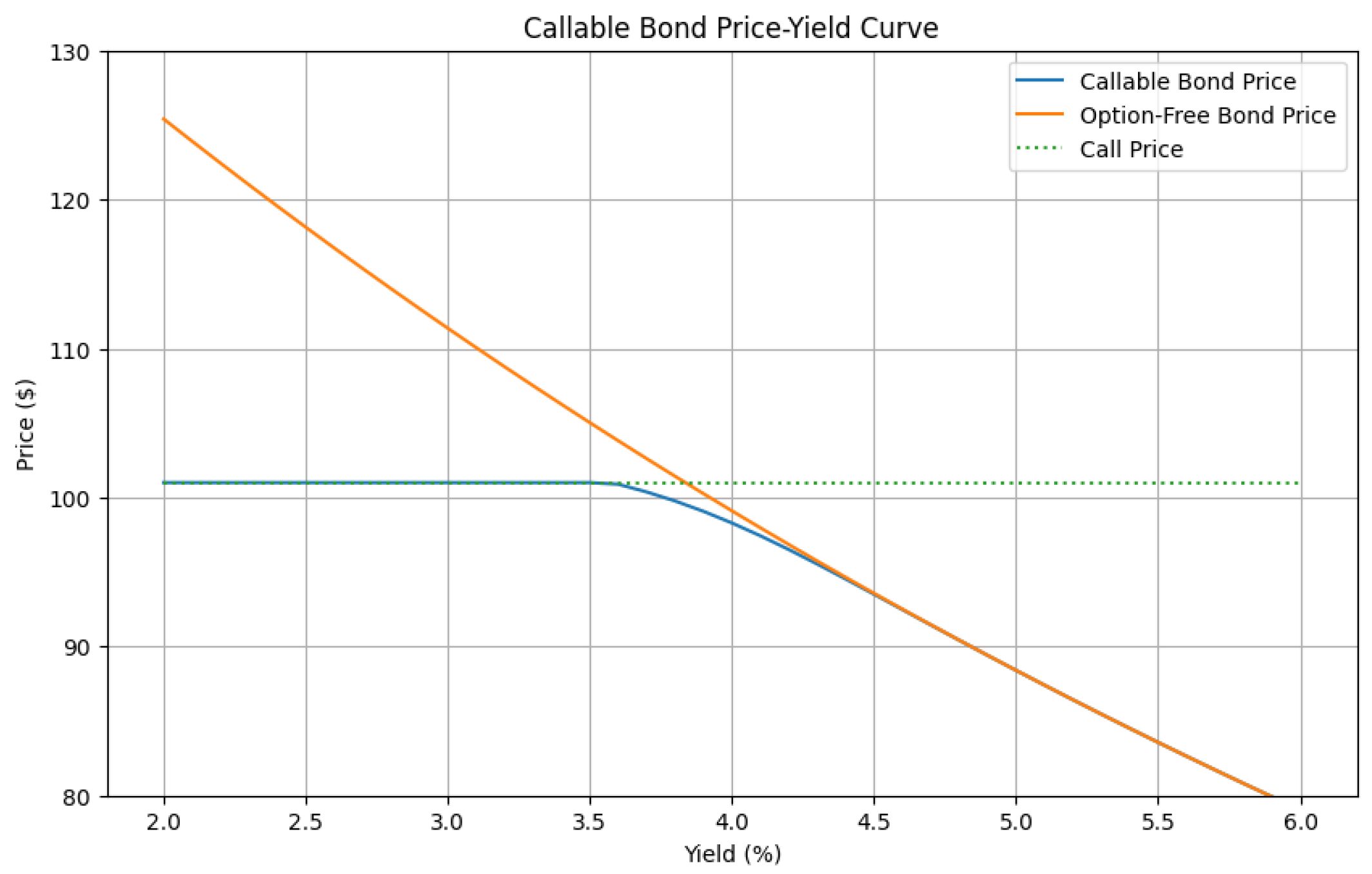
The distinctive price-yield relationship of these securities is characterized by negative convexity at low yields and positive convexity at high yields (Fabozzi 2012). This non-conventional behavior is a direct result of the embedded call option, which effectively places a cap on the bond’s price as interest rates decline. Figure 1 illustrates the contrast between callable and non-callable bonds, highlighting the impact of the call option on the bond’s price dynamics. The plot shows two 15-year, 100-par, 4% annual coupon bonds, with one of them having a call price of 101 and a call expiry of 5 years. The option volatility is set at 2% and the continuously compounded risk-free rate is assumed to be 4%. Similar bonds can currently be found as new issues or in the secondary market (e.g., CUSIP 61766YXY2, which pays semiannual coupons of 5.4% with maturity date 2 July 2040 and which can be called at par on its anniversary starting from 2030). Our calculations depend on the bond getting called by the issuer the moment its price exceeds the call price.
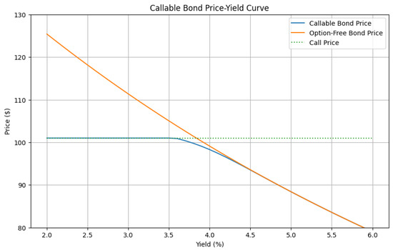
Figure 1.
Price-yield relationship for a callable and a non-callable bond. Both are 15-year, 100-par, 4% annual coupon bonds, with one of them having a call price of 101 and call expiry of 5 years. The option volatility is 2% and the continuously compounded risk-free rate is 4%.
In the context of portfolio management and risk assessment, there is a pressing need for efficient methods to price large portfolios of callable bonds, particularly when considering significant parallel shifts in the yield curve. Traditional metrics, such as duration and convexity, while useful for conventional bonds, often fall short in accurately capturing the price sensitivity of callable bonds to interest rate changes. Moreover, duration-convexity approximations, being parabolic in nature, fail to track the inflection point present in the price-yield graph of a callable bond.
Table 1 presents typical errors associated with various duration-convexity approximation methods when applied to callable bond prices for yield shifts of up to 200 basis points. The callable bond used is the 15-year bond we introduced earlier and the calculations rely on the bond’s effective duration and convexity with . Additional context on these approximation methods is provided in Orfanos (2022).

Table 1.
Approximation errors for the callable bond described in Figure 1 at yield shifts of up to 200 basis points.
By comparison, the approximation errors for an equivalent non-callable bond under the same approximation methods are negligible, as can be seen in Table 2 below.
Table 2.
Approximation errors for the non-callable bond described in Figure 1 at yield shifts of up to 200 basis points.
The limitations of standard duration and convexity approximations have motivated us to explore higher-order terms to better characterize the price dynamics of callable bonds. Recent literature has introduced the concept of ‘tilt’ (Angel et al. 2020) as a quantity of interest that can potentially provide a more comprehensive description of a bond’s behavior under varying interest rate scenarios. However, the preliminary results indicated that tilt alone does not improve the accuracy of the approximation for callable bonds.
In this paper, we add another quantity, which we have named ‘agility’, to better capture the bond’s price dynamics. Moreover, we derive explicit formulas for approximations of third and fourth order and more general formulas for approximations of any order. Still, the incorporation of bond tilt and bond agility in higher-order approximations does not always give the desired pricing accuracy. We, too, observe that while third-order approximations often improve upon second-order methods in most scenarios, they may still fail to adequately track the shape of the price-yield curve across a wide range of yield shifts. Fourth-order approximations, while potentially more accurate for smaller yield shifts (below 100 basis points) on par bonds, can, nevertheless, produce significant errors for larger shifts and premium or discount bonds.
In what follows, we propose and evaluate several additional approaches to address these challenges:
- (a)
- We discuss the role of the step size or increment h when computing these quantities.
- (b)
- We explore the effectiveness of averaging approximations of different orders.
- (c)
- We investigate the application of Padé approximants and their benefits and drawbacks.
We test our methods on a variety of callable bonds, which we have chosen to match typical agency, corporate and utilities, or municipal bond characteristics. More specifically, we consider bonds with maturity time of 5 years, time-to-call of 1 year, and bond price volatility of 2% and 4%, bonds with maturity times of 10 and 15 years, time-to-call of 5 years, and bond price volatility of 2% and 4%, and bonds with maturity times of 20 and 30 years, time-to-call of 10 years and bond price volatility of 3% and 5%. High-yield callable bonds may have a price volatility that exceeds 5% in cases of economic stress, but we do not study credit spreads, and therefore, have chosen to model volatilities that are more representative of investment-grade bonds. Furthermore, we do not vary the 4% annual coupon rate but instead consider yields of 3%, 4% and 5% to model bonds sold at a premium or discount. We also keep the call price at 101.
Our analysis could be applied to a variety of callable-like bond issues, including callable range bonds, mortgage-backed securities or collateralized debt obligations, and could also extend to other cash flow structures, such as those arising from marked-to-market financial assets, commodities, or investments that are subject to future write-downs or write-ups and could exhibit strong negative convexity. The ultimate goal, only partly realized in this paper, is to provide practitioners with reliable tools for pricing and risk management of fixed income securities with complex optionality features in cases where a full valuation approach would be infeasible or too time-consuming. The need for transparent, efficient methods that support interpretability, reproducibility, and robustness is further underscored by regulatory guidance (Basel Committee on Banking Supervision 2020; Federal Reserve System 2011), requiring all valuation approaches to be systematically validated and monitored.
While our analysis concentrates on parallel shifts in yields, it is worth noting the broader context of yield curve dynamics. The term structure of interest rates and its evolution over time have long been subjects of intense study in financial economics. Groundbreaking research in the 1990s, employing Principal Component Analysis, established that parallel shifts account for almost 90% of yield curve changes (Litterman and Scheinkman 1991). Despite the evolution of financial markets since then, more recent analyses (Barber and Copper 2012; Chen and Fu 2002) continue to support the dominant role of such shifts. The persistent explanatory power of parallel movements justifies our focus while acknowledging that future research that includes the second principal component (interpreted as the slope of the yield curve) and the third principal component (associated with the curvature of the yield curve) could provide additional insights.
Our work builds on a rich literature examining callable bond valuation and risk measurement. Early seminal works treated callable bonds as conventional bonds minus embedded call options, which is also conducted in this paper. Brennan and Schwartz (1977) extended option pricing models to explicitly model bond callability. Concurrently, Rendleman and Bartter (1980) introduced stochastic interest rate modeling, emphasizing volatility’s role in pricing debt instruments with embedded options. These frameworks paved the way for arbitrage-free term structure models, notably Ho and Lee (1986), who first calibrated no-arbitrage models to observed yield curves. Subsequently, Black et al. (1990) and Heath et al. (1992) further generalized these arbitrage-free approaches, followed by more sophisticated multi-factor models and approaches incorporating mean reversion (Hull and White 1990).
Empirical studies enhanced the understanding of callable bond risk profiles and informed risk management techniques. Dunetz and Mahoney (1988) demonstrated callable bonds’ lower effective duration and potential negative convexity. Their findings inspired further analysis by Chance (1993) of duration and convexity in other embedded option securities. Credit risk integration, not discussed in this work, also became significant, with structural models by Longstaff and Schwartz (1995) and reduced form approaches by Duffie and Singleton (1999), highlighting methods for pricing callable bonds under default risk. Practical risk management approaches emerged, including interest rate derivatives-based hedging strategies and option-adjusted spread analyses (Fabozzi 2012).
Advancements in computational methods have significantly improved callable bond valuation, although the added precision has come at the cost of computational complexity. Boyle (1977) pioneered Monte Carlo simulations for option valuation, later refined by Longstaff and Schwartz (2001). Lattice methods also evolved, notably through Hull and White (1994)’s mean-reverting interest rate lattice. Modern multi-factor models incorporating both interest rate and credit risks have addressed limitations of earlier single-factor approaches, e.g., Jarrow and Turnbull (2003). Furthermore, machine learning techniques (Becker et al. 2020; Ferguson et al. 2018) have recently augmented traditional methods, with neural networks and hybrid approaches enhancing pricing accuracy and computational efficiency but resulting in loss of interpretability.
The remainder of this paper is organized as follows: Section 2 delves deeper into the pricing characteristics of callable bonds. Section 3 reviews existing approximation methods, higher-order analogs, and their limitations. Section 4 introduces our proposed approaches and presents the results of our analysis. Section 5 consists of empirical tests for callable bonds sold at a premium or a discount, and finally, Section 6 concludes with a discussion of the implications of our findings and potential areas for future research.
2. Pricing Characteristics of Callable Bonds
Callable bonds are debt securities that grant the issuer the right, but not the obligation, to redeem the bond before its maturity date. This embedded call option typically comes with specific conditions, such as explicit call dates and call prices, that we ignore for the purposes of this article. Our focus is on the call feature, which introduces an element of optionality that fundamentally alters the bond’s risk-return profile.
As we have seen from Figure 1, the relationship between a callable bond’s price and yield is markedly different from that of a non-callable bond. Key observations from this comparison include the following:
- (a)
- As interest rates decline, the price of a callable bond approaches but does not exceed the call price. This creates a de facto ceiling on the bond’s value, represented by the flattening of the curve at lower yields.
- (b)
- In the region where the call option becomes valuable (i.e., at lower yields), the callable bond exhibits negative convexity. This means that as yields decrease, the rate of price appreciation slows down, contrary to the behavior of non-callable bonds.
- (c)
- Callable bonds typically offer a higher yield compared to similar non-callable bonds, compensating investors for the additional risk associated with the call feature.
2.1. Duration and Convexity of Callable Bonds
Our notation and definitions below come from Vaaler and Daniel (2009). P will represent the (net) present value at time 0 and v will be an annual discount factor. One exception is that we use the symbol r (instead of ) to denote the continuously compounded yield (or force of interest) in an effort to better align with existing Finance literature.
Recall that the Macaulay duration of a stream of cash flows being paid at future times is defined by
while its Macaulay convexity is given by
For callable bonds, consider the Black formula for a European call option with expiration at time t and strike K
where P is the price of the option-free bond, represents the standard normal c.d.f., and the quantities (unrelated to the Macaulay duration) are given by
with the bond price volatility and the call expiration time. The option price V is then subtracted from the option-free bond price to arrive at the price for the callable bond, also denoted by P, which is capped at the call price.
Instead of the Macaulay duration, we use the concept of effective duration, which incorporates the embedded option when considering the bond’s sensitivity to interest rate changes. The effective duration is typically lower than the Macaulay duration of a similar non-callable bond, reflecting the price ceiling imposed by the call feature. The effective duration is defined as follows:
where is the callable bond price at yield r, is the callable bond price at the initial yield , and h is the yield step size or increment.
Moreover, while non-callable bonds exhibit positive convexity throughout their price-yield curve, callable bonds display negative convexity in regions where the call option is valuable. This negative convexity implies that the bond’s price becomes less sensitive to yield decreases as yields fall. The effective convexity is given by the following:
2.2. Tilt and Agility of Callable Bonds
The careful reader will note that the equations for the effective duration and convexity depend on the first- and second-order central finite difference quotients (LeVeque 2007) as approximations to the respective derivatives in the Macaulay duration and convexity. Following this observation, Angel et al. (2020) define the Macaulay tilt as
and the effective tilt as
In this paper, we define the Macaulay agility by the equation
from which we obtain the effective agility as
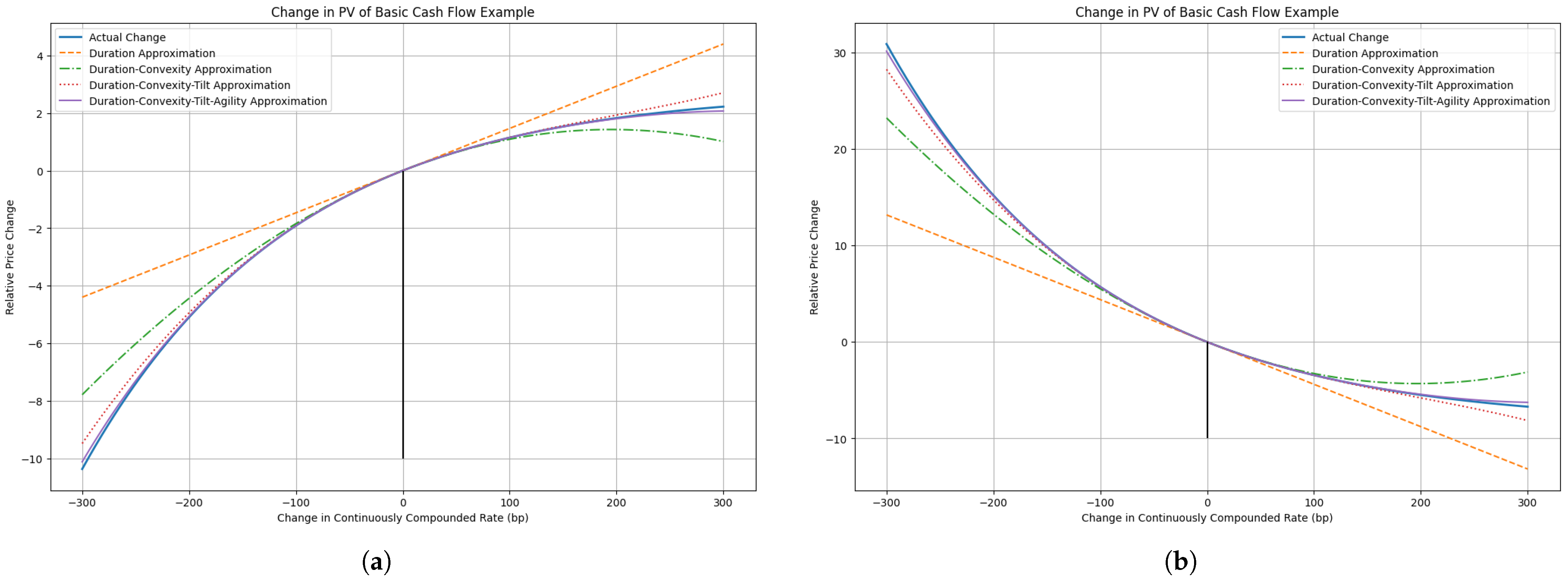
We will use a basic cash flow example to introduce these new concepts and explain our naming choice. Start with a payment of 1 at time 1 and a payment of at time 50. It can be readily computed that at a continuously compounded rate of 2%, the net present value at time 0 is . Furthermore, all quantities of interest at time 0 are negative, as can be seen in Table 3.
Table 3.
Price, effective duration, effective convexity, effective tilt, and effective agility at time 0 for a basic cash flow example. Computed using .
In subsequent sections, we will discuss various higher-order approximations in great detail. The purpose of Figure 2a is to showcase the effect of adding each successive term to an approximation formula. More specifically,
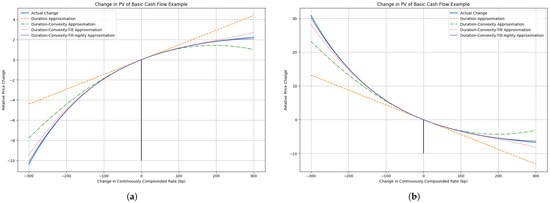
Figure 2.
Understanding the effect of tilt and agility. (a) Both are negative. (b) Both are positive.
- (a)
- The addition of a convexity term to the duration approximation results in an arched price-yield curve that tracks the actual change in PV more closely.
- (b)
- The addition of a tilt term to the duration-convexity approximation has the effect of twisting the price-yield curve counterclockwise without altering the tangent line. This illustrates why ‘tilt’ is an appropriate name for this quantity.
- (c)
- Finally, the addition of an agility term to the duration-convexity-tilt approximation provides the best match to the actual PV change by bending the price-yield curve downward, thus affecting the responsiveness of the price to larger changes in the interest rates. The increased responsiveness explains the choice of the term ‘agility’.
We now change the time-50 cash flow from to . At the same continuously compounded rate, the net present value at time 0 becomes , while all quantities of interest are now positive and given in Table 4. A quick look at Figure 2b will convince the reader that
Table 4.
Price, effective duration, effective convexity, effective tilt, and effective agility at time 0 for a basic cash flow example. Computed using .
- (a)
- Positive tilt corresponds to a clockwise twist of the price-yield curve.
- (b)
- Positive agility is associated with bending the price-yield curve upward.
The above figures seem to suggest that we always obtain better approximations by incorporating higher-order terms, but this is not necessarily true for complicated cash flows such as callable bonds. Extending the range of the yield shifts would reveal the divergent behavior of these approximations, with the rate of divergence increasing with the approximation order. This will be illustrated in the next section when discussing realistic examples of callable bonds.
2.3. The Role of the Step Size h
The calibration of h has practical significance that may not be apparent at first sight. Setting h as a very small increment (e.g., 1 basis point) produces a close fit to the mathematical derivative and, thus, to the Macaulay duration, and likewise for higher-order derivatives. As a result, all prices used are in the neighborhood of the current price and less pricing information is captured, especially in the following cases:
- when the current price falls inside the ‘flat’ call price part of the price-yield curve, corresponding to lower yields;
- when the current price falls inside the non-callable part of the price-yield curve, corresponding to higher yields.
In such situations, approximations of any order will fail to track the price-yield curve in its entirety. On the other hand, a larger value for h (e.g., 100 basis points) will be more likely to contain information about the bond as well as the call option characteristics but at the cost of reduced accuracy. As we will see later, sacrificing precision to increase the information reflected in the effective duration, effective convexity, effective tilt and effective agility will pay dividends when attempting to approximate the price-yield curve of callable bonds.
3. Approximation Methods for Callable Bonds
The complex price dynamics of callable bonds, as discussed earlier, necessitate sophisticated valuation techniques. However, the computational intensity of full option-adjusted valuation models can be prohibitive, especially when dealing with large portfolios or in real-time trading environments, thus creating the need for more efficient pricing algorithms. Modern machine learning techniques, such as neural networks, have reduced the computational cost and improved the accuracy of the model but suffer from opaqueness in most implementations.
Efficient and easily validated pricing methods are crucial in portfolio management since large institutional portfolios may contain thousands of callable bonds, requiring rapid valuation for risk assessment and portfolio optimization. Trading and market-making in fast-moving markets is another potential area of application, given that traders need quick, reliable pricing estimates to make informed decisions. Finally, stress testing and scenario analysis often involve evaluating portfolio performance under various interest rate shifts, demanding computationally efficient methods. In addition, ‘black box’ methods often need to be accompanied by more transparent computations when defending capital and reserve estimates to regulators. To achieve greater computational efficiency and maintain interpretability and transparency while keeping errors under control, we turn to classical approximation methods.
3.1. Lower-Order Approximation Methods
The following approximation methods have appeared in the literature.
- First-order approximation from Barber (1995):
- second-order approximation from Fischer and Weil (1971):
- second-order approximation from Tchuindjo (2008):
- second-order approximation from Alps (2017):
- second-order approximation from Orfanos (2022):
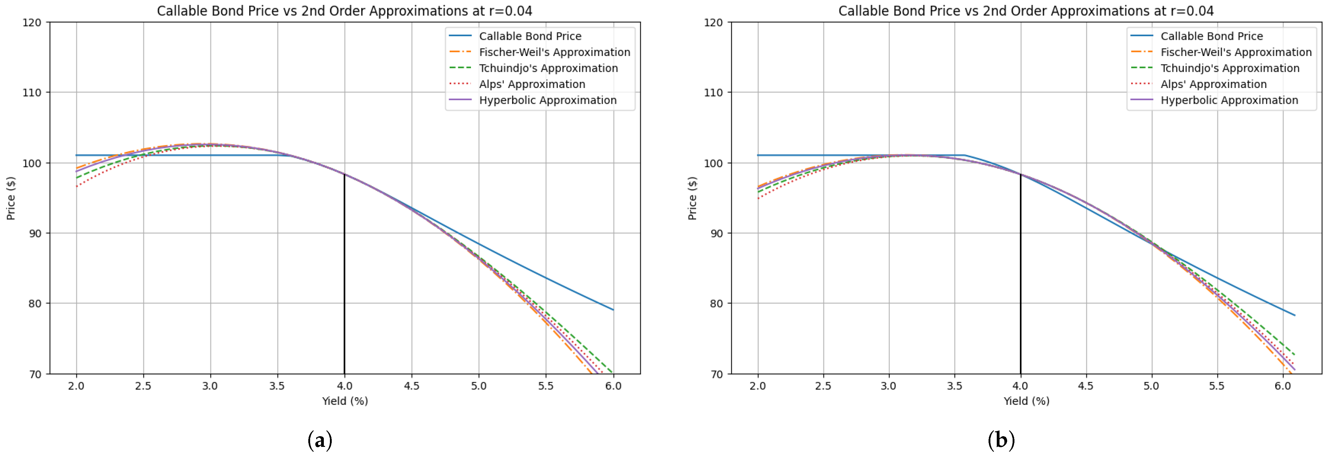
As demonstrated in Table 1 and Table 2, these approximations are satisfactory when evaluating conventional bond portfolios but prove inadequate in the presence of optionality. See Figure 3 for a visual comparison of these approximation methods when applied to the same 15-year callable bond as before.
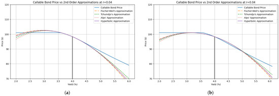
Figure 3.
Second-order approximation methods for the callable bond described in Figure 1. (a) . (b) .
3.2. Higher-Order Approximation Methods
The derivation of a third or fourth-order version of Fischer–Weil’s approximation formula is fairly straightforward, but the same cannot be said for the higher-order versions of approximations by Tchuindjo, Alps, or the hyperbolic approximation. In this section, we present the generalizations of these approximation formulas and refer the interested reader to Appendix A and Appendix B for the mathematical derivations.
- Fischer–Weil’s fourth-order approximation:
- Barber–Tchuindjo’s fourth-order approximation:
- Alps’ fourth-order approximation:
- The third-order hyperbolic approximation:
- The fourth-order hyperbolic approximation:
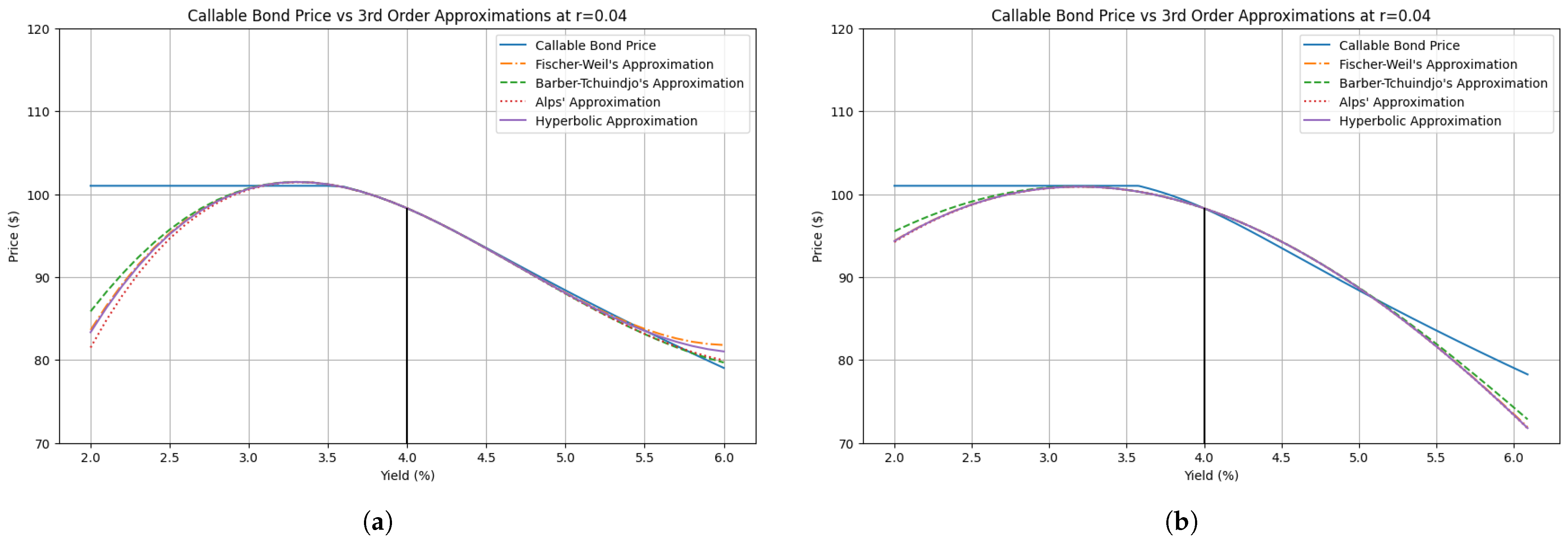
3.3. The Paradox of Higher-Order Approximations
The data do not support our initial hypothesis that higher-order approximations always track the price-yield curve more closely. Interestingly,
- (a)
- Third-order approximations, while improving upon second-order methods for positive yield shifts, do worse for negative yield shifts, especially for small increments h. Figure 4a shows that third-order approximations have absolute errors between 15 and 20% for a −200 bps yield shift, when the corresponding errors for the second-order methods shown in Figure 3a are all less than 5%.
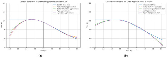 Figure 4. Third-order approximation methods for the callable bond described in Figure 1. (a) . (b) .
 - (b)
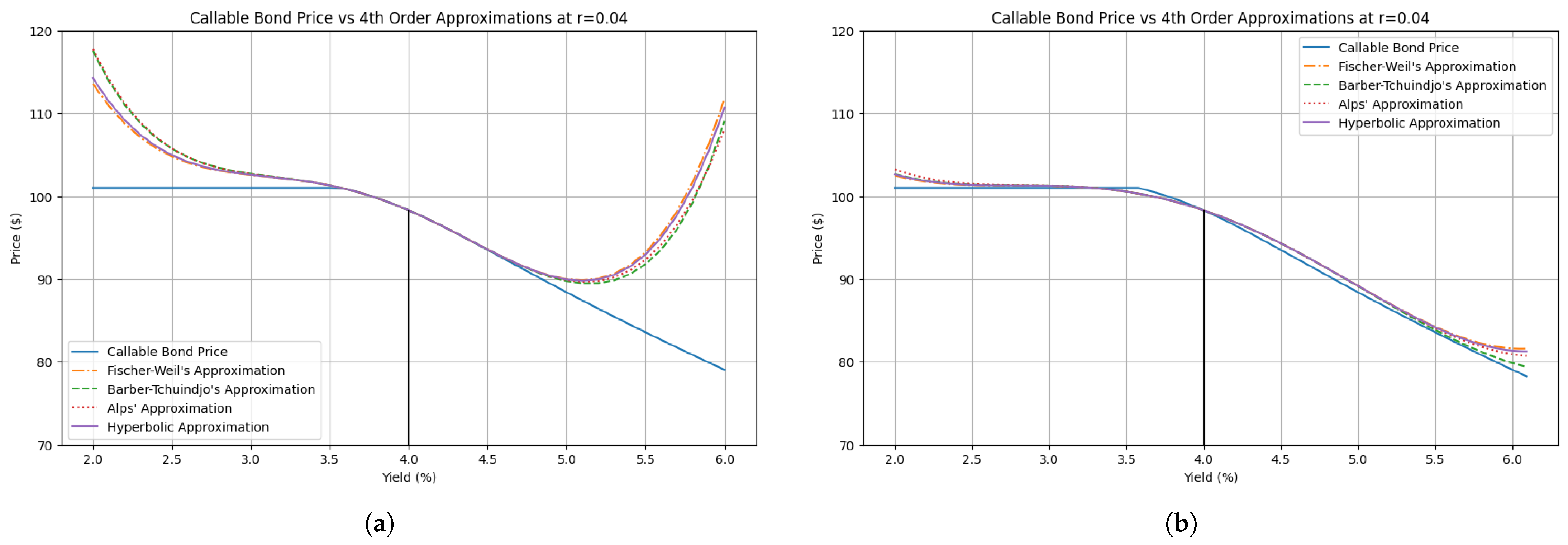
- Fourth-order approximations show improved accuracy for smaller yield shifts (<100 bps) but can produce significant errors for larger shifts, often performing worse than lower-order approximations, especially for small increments h. For example, the absolute errors shown in Figure 5a are all larger than 12% for the same −200 bps yield shift.
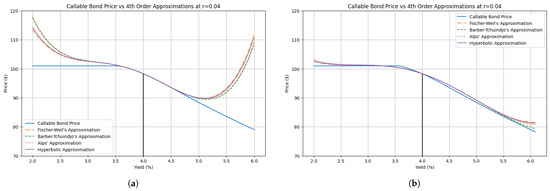 Figure 5. Fourth-order approximation methods for the callable bond described in Figure 1. (a) . (b) .
 - (c)
- The correct calibration of h is significantly more consequential than the choice of fourth-order approximation.
Figure 4 and Figure 5 show how different order approximations perform under various yield shifts. The approximations are applied to the 15-year callable bond introduced earlier and show a limited radius of convergence for but also great promise in the case of . Figure 5b suggests that the Barber–Tchuindjo approximation may provide the best fit, at least for positive yield shifts and for this specific bond. In Table 5, we summarize the approximation errors for all four fourth-order approximations when .
Table 5.
Approximation errors for the callable bond described in Figure 1 at yield shifts of up to 200 basis points with .
4. Building Improved Approximations
Although the aforementioned fourth-order approximations perform remarkably well when , they do not reach the level of precision that lower-order methods have when approximating non-callable bonds. Below, we discuss two methods that are intended to capture more effectively the complex behavior of callable bonds and thus result in smaller errors while maintaining computational efficiency and explicitness.
4.1. Averaged Order Approximations
Our first proposed approach involves averaging the second through fourth-order approximations as an attempt to cancel out errors and produce better estimates. Lower-order approximations generally display more stable behavior across all yield shifts, while higher-order methods are more accurate within a narrower range of yield shifts that are more likely to happen.
Let , , and represent the prices obtained from the second-, third-, and fourth-order hyperbolic approximations, respectively. The averaged approximation is simply given by the following:
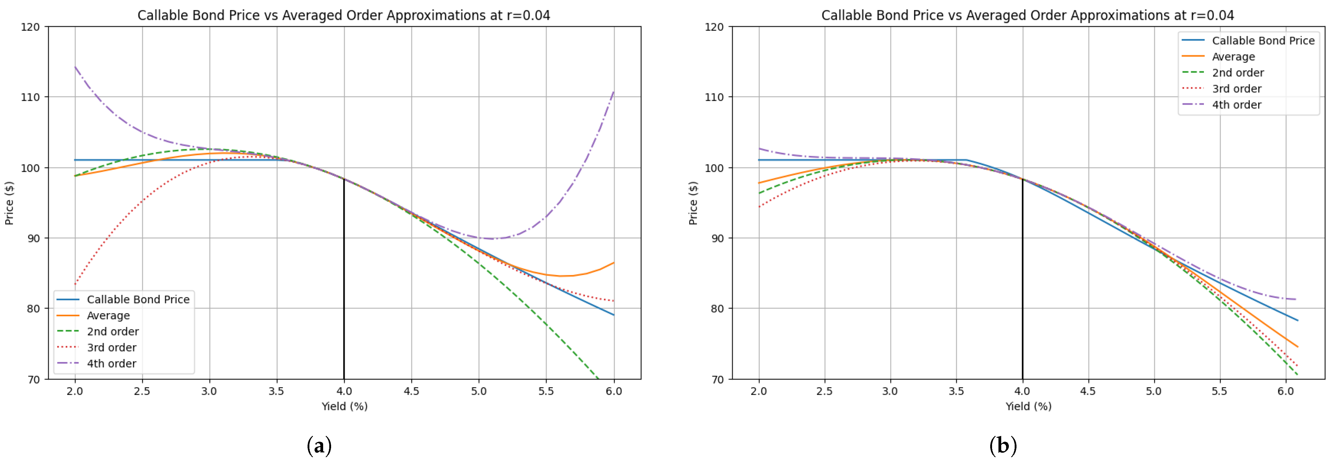
The choice of using the hyperbolic approximations for this construction is arbitrary, and the same idea could be applied equally well to another family of approximations. Figure 6 gives a visual comparison of the averaged order approximation vs. its components. Although appears to perform worse than the fourth-order hyperbolic approximation for , we will see later on that averaging approximations of different orders has advantages for yield shifts that are not too large.
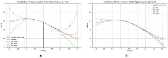
Figure 6.
Averaged-order hyperbolic approximations for the callable bond described in Figure 1. (a) . (b) .
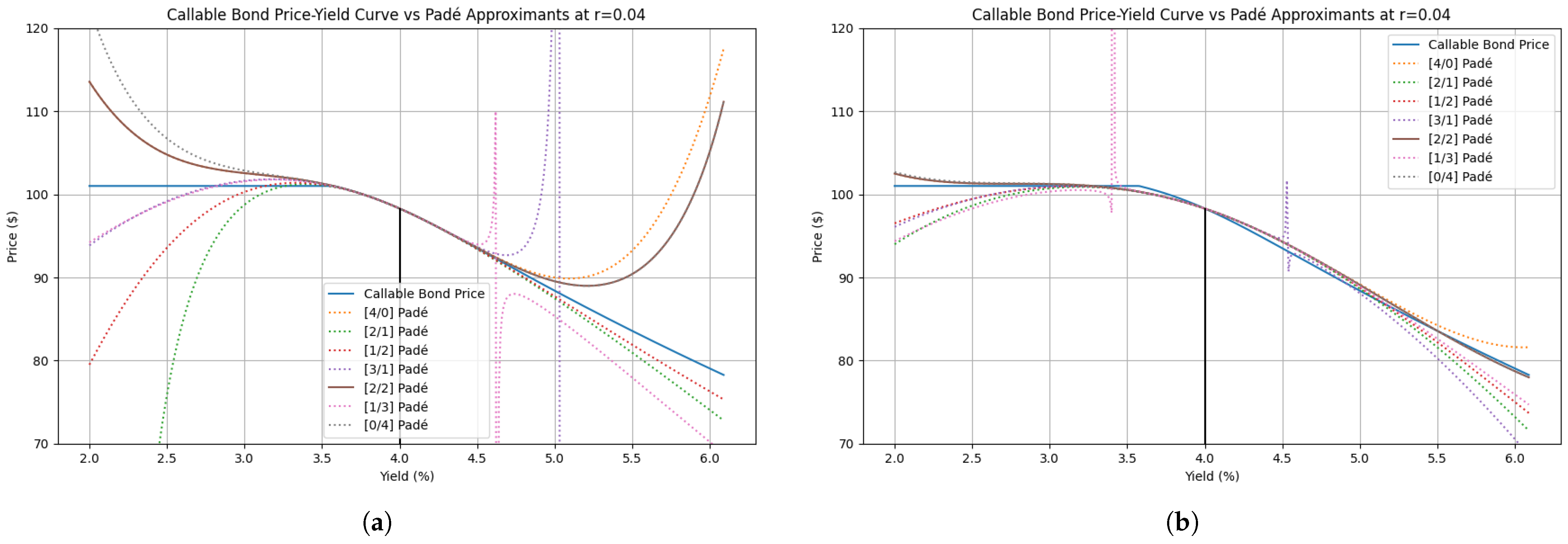
4.2. Padé Approximants
The next approach leverages Padé approximants, which are well-known rational function approximations that often capture complex behaviors more effectively than polynomial approximations. On the flip side, the denominators introduce spurious poles (i.e., mathematical singularities) that can produce nonsensical results at certain yields.
More specifically, a Padé approximant of order for the price function takes the following form:
with ’s and ’s computed from the equations , . Readers can find a derivation of the [2/2] Padé approximant based on the Fischer–Weil approximation in Appendix C in lieu of a more extensive treatment of this theory. Various Padé approximants and their proximity to the price-yield graph of the callable bond are shown in Figure 7 below. The same figure also shows how the choice of h affects the occurrence and position of poles.
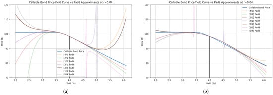
Figure 7.
Padé approximants for the callable bond described in Figure 1. Two distinct poles are evident in each figure. (a) . (b) .
It is known (Baker 1975) that diagonal Padé approximants typically exhibit the best behavior, which agrees with empirical evidence from using these approximants in the context of callable bond price estimation.
4.3. Results for All Callable Bonds
Table 6 compares the fourth-order Barber–Tchuindjo approximation to the averaged order hyperbolic approximation and to the [2/2] Padé approximant across all yield shifts for each of the bonds introduced at the beginning of this article. Various bonds are coded by the triple , where T refers to the bond’s maturity time in years, is the time-to-call, and is the bond’s price volatility. As before, .
Table 6.
Summary of approximation errors of the fourth-order Barber–Tchuindjo (BT4) approximation, the averaged order hyperbolic (AveH) approximation, and the [2/2] Padé approximant for various callable bonds. The triple consists of the bond’s maturity time in years, the time-to-call, and the bond’s price volatility. All bonds have been priced at a continuously compounded yield .
5. Premium and Discount Bonds
So far, we have tested a number of approximation formulas on a bond that was roughly sold at par, i.e., with a coupon rate (assumed annual effective) that was numerically equal to the prevailing yield rate (continuously compounded). But do our results hold the same if we assume the bond’s yield is substantially lower or higher than its coupon rate?
For small values of h, our approximations perform worse when applied to callable bonds where the option is either deep in the money or out of the money. As explained earlier, a sizable increment h is essential if we want full information about the callable bond reflected in the calculation of its effective duration, effective convexity, etc. Still, premium bonds that approximate the call price can end up mispriced under the assumption of a large positive yield shift, and conversely, discount bonds may not be well estimated if yields drop to such an extent that the bond is now on the verge of being called early by the issuer.
The calculations in Table 7 and Table 8 serve to reassure the reader that our approximations are robust in these cases as well. This is important because, while new issues may typically be sold at par, a more realistic portfolio of callable bonds issued at different times and with different coupon rates may include both premium and discount bonds and will, therefore, behave in a more nuanced way than the examples discussed so far.
Table 7.
Summary of approximation errors of the fourth-order Barber–Tchuindjo (BT4) approximation, the averaged order hyperbolic (AveH) approximation, and the [2/2] Padé approximant for various callable bonds. The triple consists of the bond’s maturity time in years, the time-to-call, and the bond’s price volatility. All bonds have been priced at a continuously compounded yield .
Table 8.
Summary of approximation errors of the fourth-order Barber–Tchuindjo (BT4) approximation, the averaged order hyperbolic (AveH) approximation, and the [2/2] Padé approximant for various callable bonds. The triple consists of the bond’s maturity time in years, the time-to-call, and the bond’s price volatility. All bonds have been priced at a continuously compounded yield .
6. Conclusions
In this paper, we examined the challenges of accurately approximating the price-yield relationship of callable bonds, whose embedded options give rise to nonlinear behavior that cannot be adequately captured by standard duration-convexity measures. While higher-order terms—bond tilt and agility—expand the flexibility of known approximations, our empirical findings indicate that merely increasing the order of Taylor-like expansions does not, by itself, guarantee improved accuracy across a wide range of yield shifts. In fact, both third- and fourth-order approximations may underperform second-order methods in certain market conditions, especially when yields move substantially away from par.
We proposed and tested two alternative approaches to mitigate these shortcomings: (i) averaging higher-order hyperbolic approximations, and (ii) leveraging Padé approximants—specifically, the [2/2] type. As shown in Table 9, our methods (using ) performed reliably for yield shifts of up to 200 basis points, achieving mean absolute errors below 2.5% under all circumstances. In particular,
Table 9.
Mean absolute errors of the fourth-order Barber–Tchuindjo (BT4) approximation, the averaged order hyperbolic (AveH) approximation, and the [2/2] Padé approximant for various types of callable bonds.
- (a)
- All three approximation methods performed exceptionally well for agency bonds, which typically have shorter maturities and call dates. Errors are below 0.5% regardless of which approximation method was used. Corporate/utility bonds and especially longer-term municipal bonds produced moderately higher errors, depending on the method.
- (b)
- The [2/2] Padé approximant exhibited better accuracy than the Barber–Tchuindjo approximation for large yield shifts. No poles were detected across all bond types and yield shifts. Moreover, the averaged-order hyperbolic approximation gave the best results for yield shifts inside the −150 bps to 100 bps range.
- (c)
- An unexpected result is that ±50 bps yield shifts sometimes produce larger errors than ±100 bps shifts. This is a consequence of sacrificing local precision by using a relatively high value for h to achieve better overall performance.
Unsurprisingly, neither technique approached the level of precision that can be obtained for non-callable bonds, despite the improved performance of these averaged or Padé-based methods. However, this unrealistic goal should not detract from the fact that these approximation methods performed fairly well across the board. Having said that, we feel obliged to reiterate that a single approximation cannot perfectly capture all the nuances of callable bonds in all market environments. Instead, a toolkit approach that combines multiple approximations, averaging their outputs, or “splicing” them together with well-chosen tail behaviors can yield robust pricing estimates for large portfolios without resorting to full stochastic option-adjusted or machine learning models.
Several directions remain open for future research. First, incorporating dynamic yield curve shifts beyond parallel moves (e.g., slope or curvature changes) may enhance the realism of stress tests and scenario analyses. Second, adapting these approximations to mortgage-backed securities or other prepayable instruments that are also susceptible to duration extension for higher yields could illuminate whether higher-order metrics like tilt and agility improve sensitivity estimates for embedded prepayment risk. Moreover, investigating the possibility of poles for the [2/2] Padé approximant would provide added clarity on the reliability of this method. Lastly, estimating the computational complexity of these formula-based methods and comparing it with the complexity of data-driven approximation techniques or the computational time required for full valuation could add practical relevance to any future work. We hope that the proposed methods will stimulate further developments in both theoretical modeling and practical applications for managing interest rate risk in complex fixed-income portfolios.
Author Contributions
Conceptualization, S.S.D. and S.C.O.; methodology, S.S.D. and S.C.O.; original draft preparation, S.C.O.; revisions, S.C.O. All authors have read and agreed to the published version of the manuscript.
Funding
This research received no external funding.
Data Availability Statement
The raw data supporting the conclusions of this article will be made available by the authors on request.
Acknowledgments
The authors express their sincere gratitude to the anonymous reviewers whose thoughtful feedback and detailed suggestions significantly improved the quality of this manuscript.
Conflicts of Interest
The authors declare no conflicts of interest.
Appendix A. Approximation Formulas of Higher Order and Their Derivation
Several of the known approximations are slight variations of the same general construction. Below, we provide details on how one could obtain these approximations in full generality.
Given the force of interest r, the net present value of a series of cash flows paid at discrete times ; is given by the following:
thus,
for ease of notation, define the following:
and observe that it is a linear operator:
therefore,
We now consider the following cases:
- Fischer–Weil’s nth-order approximation: Substitute the nth-order Taylor polynomial of the exponential function in the bracket and use linearity to deriveBy letting , , , and , we obtain the fourth-order approximation
- Barber–Tchuindjo’s nth-order approximation: We take the natural logarithm of (A1):wherewith denoting partial Bell polynomials. More concretely, the first few terms are as follows:etc. This results in the following fourth-order approximation formula, which generalizes both Barber’s and Tchuindjo’s approximations:Alternatively, we can manipulate (A1) in the following way:where . Then, replace the exponential term inside the bracket with its nth degree Maclaurin polynomial to obtainThis yields a slightly different fourth-order approximation:
- nth-order Alps’ Approximation: This time, express (A5) as a function of the effective rate of interest i:and substitute the nth-order Taylor polynomial inside the bracket to obtainWe now switch back to r:The last bracket can be further simplified after noting that the product inside it equals , where are the unsigned Stirling numbers of the first kind.Finally, the fourth-order approximation is as follows:
Appendix B. Using the Laplace Transform to Generalize the Hyperbolic Approximation Formula
We consider the linear ordinary differential equation:
with initial conditions:
Our goal is to solve this ODE using the Laplace transform, which is a concept analogous to moment-generating functions for probability distributions.
Let . Applying the Laplace transform to our ODE gives the following:
That, in turn, yields the following solution in the frequency domain:
To switch back to the time domain, we will need to simplify the expression on the right-hand side using partial fraction decomposition before applying the inverse Laplace transform. Let be the nth roots of unity. Then,
and we can write in the form
where are constants to be determined. The solution to our ODE in the time domain is then
It remains to compute the ’s. Observe that
from the initial conditions, which implies that
After some simplifications, this boils down to
for . Note that if we had instead of and we wanted to evaluate at , then the left-hand side of the above equation would be
Substituting back into (A10), we obtain
after replacing with .
The next step is to derive the third-order and fourth-order approximations (unlike previous approximation formulas, the third-order approximation is not an obvious part of the fourth-order approximation). For we have the following:
which, after collecting terms, gives
Below, we show that the answer is real-valued. Note that and thus,
Use Euler’s formula to expand the exponential terms to
followed by the cancellation of the imaginary parts, resulting in
We leave it to the reader to verify that
On the other hand, for we obtain the following:
After canceling out terms, we have the following:
Appendix C. The [2/2] Padé Approximant
The calculation that follows can be adapted to compute the coefficients of Padé approximants of other orders.
Starting from with the following derivatives at :
Consider the Taylor series expansion of around 0 up to the fourth order:
For convenience, define the following:
A Padé approximant has the following form:
We want to determine and so that matches up to terms of order . Multiplying out
and expanding the right side up to gives
Equating coefficients, we obtain the following system:
The last two equations allow us to solve for and in terms of the duration, convexity, tilt and agility:
Solving this system, we find the following:
We now compute from the remaining equations, with the final answer being the following:
Overall
References
- Alps, Robert. 2017. Using Duration and Convexity to Approximate Change in Present Value. SOA Financial Mathematics Study Note FM-24-17, pp. 1–18. Available online: https://www.soa.org/globalassets/assets/Files/Edu/2017/fm-duration-convexity-present-value.pdf (accessed on 1 January 2025).
- Angel, James, Jiadi Chen, and Nikkie Pacheco. 2020. First Duration, Then Convexity, Then What? Tilt? Working paper, Georgetown University McDonough School of Business. Available online: https://ssrn.com/abstract=3697547 (accessed on 1 January 2025).
- Baker, George Allen. 1975. Essentials of Padé Approximants. Cambridge: Academic Press. [Google Scholar]
- Barber, Joel. 1995. A Note on Approximating Bond Price Sensitivity Using Duration and Convexity. The Journal of Fixed Income 4: 95–98. [Google Scholar] [CrossRef]
- Barber, Joel, and Mark Copper. 2012. Principal Component Analysis of Yield Curve Movements. Journal of Economics and Finance 36: 750–65. [Google Scholar] [CrossRef]
- Barth, Daniel, Jay Kahn, Phillip Monin, and Oleg Sokolinskiy. 2024. Reaching for Duration and Leverage in the Treasury Market. Finance and Economics Discussion Series 2024-039. Washington, DC: Board of Governors of the Federal Reserve System. [Google Scholar] [CrossRef]
- Basel Committee on Banking Supervision. 2020. Supervisory Guidance for Assessing Banks’ Financial Instrument Fair Value Practices. Basel: Bank for International Settlements. [Google Scholar]
- Becker, Sebastian, Patrick Cheridito, and Arnulf Jentzen. 2020. Deep optimal stopping. Journal of Machine Learning Research 21: 1–36. [Google Scholar]
- Black, Fischer, Emanuel Derman, and William Toy. 1990. A One-Factor Model of Interest Rates and its Application. Financial Analysts Journal 46: 33–39. [Google Scholar] [CrossRef]
- Boyle, Phelim. 1977. Options: A Monte Carlo Approach. Journal of Financial Economics 4: 323–38. [Google Scholar]
- Brennan, Michael, and Eduardo Schwartz. 1977. Savings Bonds, Retractable Bonds and Callable Bonds. Journal of Financial Economics 5: 67–88. [Google Scholar] [CrossRef]
- Chance, Don. 1993. Convertibles and Duration Analysis. Financial Analysts Journal 49: 35–43. [Google Scholar]
- Duffie, Darrell, and Kenneth Singleton. 1999. Modeling Term Structures of Defaultable Bonds. Review of Financial Studies 12: 687–720. [Google Scholar] [CrossRef]
- Dunetz, Mark, and James Mahoney. 1988. Using Duration and Convexity in the Analysis of Callable Bonds. Financial Analysts Journal 44: 53–72. [Google Scholar]
- Fabozzi, Frank, ed. 2012. The Handbook of Fixed Income Securities, 8th ed. New York: McGraw-Hill. [Google Scholar]
- Federal Reserve System. 2011. SR 11-7: Guidance on Model Risk Management. Washington, DC: Board of Governors of the Federal Reserve System. [Google Scholar]
- Ferguson, Raymond, Andrew Green, and Martin Schweizer. 2018. Deeply Learning Derivatives. Available online: https://ssrn.com/abstract=3291285 (accessed on 1 January 2025).
- Fischer, Lawrence, and Roman Weil. 1971. Coping with the Risk of Interest-Rate Fluctuations: Returns to Bondholders from Naive and Optimal Strategies. The Journal of Business 44: 406–31. [Google Scholar]
- Heath, David, Robert Jarrow, and Andrew Morton. 1992. Bond Pricing and the Term Structure of Interest Rates: A New Methodology. Econometrica 60: 77–105. [Google Scholar]
- Ho, Thomas, and Sang-Bin Lee. 1986. Term Structure Movements and Pricing Interest Rate Contingent Claims. Journal of Finance 41: 1011–29. [Google Scholar]
- Hull, John, and Alan White. 1990. Pricing Interest-Rate Derivative Securities. Review of Financial Studies 3: 573–92. [Google Scholar]
- Hull, John, and Alan White. 1994. Numerical Procedures for Implementing Term Structure Models. Journal of Derivatives 2: 7–16. [Google Scholar]
- Jarrow, Robert, and Stuart Turnbull. 2003. Derivative Securities. Mason: Thomson/South-Western. [Google Scholar]
- Jian, Chen, and Michael Fu. 2002. Hedging beyond Duration and Convexity. Paper presented at Winter Simulation Conference, San Diego, CA, USA, 8–11 December 2002; Edited by Enver Yücesan, Chun-Hung Chen, Jane Snowdon and John Charnes. pp. 1593–99. [Google Scholar]
- LeVeque, Randall. 2007. Finite Difference Methods for Ordinary and Partial Differential Equations. Philadelphia: Society for Industrial and Applied Mathematics. [Google Scholar]
- Litterman, Robert, and José Scheinkman. 1991. Common Factors Affecting Bond Returns. Journal of Fixed Income 1: 54–61. [Google Scholar] [CrossRef]
- Longstaff, Francis, and Eduardo Schwartz. 1995. A Simple Approach to Valuing Risky Fixed and Floating Rate Debt. Journal of Finance 50: 789–819. [Google Scholar] [CrossRef]
- Longstaff, Francis, and Eduardo Schwartz. 2001. Valuing American Options by Simulation: A Simple Least-Squares Approach. Review of Financial Studies 14: 113–47. [Google Scholar]
- Orfanos, Stefanos. 2022. A Comparison of Macaulay Approximations. Risks 10: 153. [Google Scholar] [CrossRef]
- PIMCO. 2024. Valuing Callable Municipal Bonds. Available online: https://www.pimco.com/us/en/resources/education/valuing-callable-municipal-bonds (accessed on 1 January 2025).
- Rendleman, Richard, and Brit Bartter. 1980. The Pricing of Options on Debt Securities. Journal of Financial and Quantitative Analysis 15: 11–24. [Google Scholar] [CrossRef]
- Schwab, Charles. 2024. Callable Bonds: Understanding How They Work. Available online: https://www.schwab.com/learn/story/callable-bonds-understanding-how-they-work (accessed on 1 January 2025).
- Tchuindjo, Leonard. 2008. An Accurate Formula for Bond-Portfolio Stress Testing. The Journal of Risk Finance 9: 262–77. [Google Scholar]
- Tucker, Matthew, and Jared Murphy. 2013. The Impact of Negative Convexity When Rates Change: How Corporate Bonds Can Diversify an MBS Portfolio. Available online: https://www.bankdirector.com/wp-content/uploads/Negative_Convexity_Whitpaper.pdf (accessed on 1 January 2025).
- Vaaler, Leslie, and James Daniel. 2009. Mathematical Interest Theory, 2nd ed. Washington, DC: Mathematical Association of America. [Google Scholar]
Disclaimer/Publisher’s Note: The statements, opinions and data contained in all publications are solely those of the individual author(s) and contributor(s) and not of MDPI and/or the editor(s). MDPI and/or the editor(s) disclaim responsibility for any injury to people or property resulting from any ideas, methods, instructions or products referred to in the content. |
© 2025 by the authors. Licensee MDPI, Basel, Switzerland. This article is an open access article distributed under the terms and conditions of the Creative Commons Attribution (CC BY) license (https://creativecommons.org/licenses/by/4.0/).