Fuzzy Non-Payment Risk Management Rooted in Optimized Household Consumption Units

Abstract

Traditionally, business risk management models have not taken into consideration household composition for the purposes of credit granting or project financing in order to manage the risk of default. In this research, an improvement in the risk management model was obtained by introducing household composition as a new exogenous variable. With the application of generalized reduced gradient nonlinear optimization modeling, improved consumption units are determined according to the different types of household size and the age of their members. Estimated household economies of scale show a consistent pattern even in the year 2020, corresponding with the COVID-19 outbreak. Thus, an adjusted estimation of the household equivalized disposable income is obtained. Based on this more accurate equivalized income estimation, acceptable debt levels can be determined. The estimation of probabilities of default allows the household risk of default to be managed. In this way, a novel model is proposed by incorporating household composition into credit risk evaluation using fuzzy clustering and optimization techniques. Companies can assess the expected loss of a credit exposure through a model that can help them in the process of making evidence-informed decisions.

1. Introduction

In recent years, there has been increasing interest in research on business risk management, particularly after the financial crisis that took place in the late 2000s (Bessis 2015). In general, risk management evaluations (Zhao et al. 2015) require the identification, assessment, and control of any of an institution’s risks, particularly credit risks. There are multiple generations of models for assessing credit risk (Chen et al. 2016) and estimating default probabilities (Leland 2012), but the application of household consumption units derived from household composition is not usually considered in any of these models as an exogenous variable.

In this context, it is necessary to highlight that significant differences are found in the main household economic variables depending on the age group composition. These differences in median incomes by large age groups exceed 15% in the EU-27 and even surpass 20% in countries like Germany when comparing people of working age (16 to 64 years) with older people (65 years and over). This is evidence that must undoubtedly be taken into account when proceeding with the study, analysis, and evaluation of household credit risks or default probabilities.

In the EU, the AI Act has recently come into force. This Act is one of the first regulatory frameworks for AI worldwide. The new regulation requires that discriminatory outcomes, which could be based on personal characteristics such as age or place of residence, must be avoided. Additionally, it explicitly considers credit risk assessment systems as high-risk situations that could affect fundamental human rights (Mazzini and Bagni 2023). Therefore, credit assessment systems must comply with these stringent criteria to be used in the EU.

This compliance context necessitates the enhancement of credit risk assessment systems (Nkambule et al. 2024) to mitigate potential biases. These biases may stem from data, where individual information could not be well captured or represented, or from algorithms, particularly if some personal characteristics are not adequately reflected. Such biases could result in discriminatory and thus unfair outcomes in financial risk management (Fritz-Morgenthal et al. 2022). A biased outcome from a credit risk assessment, affecting a specific group and leading to an unjust or unmotivated denial of credit, could be understood as discrimination, which the regulation expressly prohibits (Weber et al. 2024).

Bearing in mind this situation, based on empirical data obtained from official sources, this research proposes a refined statistical model by incorporating household composition into credit risk evaluation. This model, which is rooted in the calculation of optimized household consumption units from official statistics, allows businesses a more direct estimation of default probabilities as well as the expected losses for credit risk. In this way, businesses can more easily estimate the expected credit risk loss, simplifying their calculations and facilitating a periodic and simultaneous update with official information sources, taking into account any changes in household composition, income, and consumption patterns.

Literature Review

A particularly necessary line of research in the evaluation of household credit risk (Fisher 2019) is the incorporation of demographic variables (Wang and Mao 2023) such as age, family composition, gender, and place of residence in the risk analysis (Ampountolas et al. 2021). In this context, big data analysis (Chang et al. 2024) must overcome the challenge of sample composition, which requires the results obtained to be adjusted in cases where the available data are biased or unrepresentative (Brygała 2022).

Fuzzy systems are playing an increasingly important role in multiple areas of knowledge (Bahoo et al. 2024). These systems can solve practical clustering problems by operationally incorporating personal variables into models, offering better results than conventional models (Milana and Ashta 2021) and expanding classification methods (Baser et al. 2023). Many of the improvements of these models have been empirically identified, especially regarding the prevention of financial crises or defaults (Sanchez-Roger et al. 2019). Fuzzy systems (Wójcicka-Wójtowicz and Piasecki 2021) are gaining prominence (Alonso Moral et al. 2021) due to their potential application in improving the interpretability and explanatory power of modern artificial intelligence systems (Černevičienė and Kabašinskas 2024). One of their main advantages is their transparency and ability to model imprecise information derived from big data to improve decision-making processes and credit risk assessment (Salazar and Figueroa-García 2025).

Recent studies have identified significant improvements in reducing credit default rates (Bermudez Vera et al. 2025) by incorporating data analysis methodologies instead of traditional methods (Nahar et al. 2024). The ability to identify complex patterns and correlations dynamically over time enables predictive analysis for monitoring and measuring credit risks (Wang et al. 2024) beyond the historical evaluation at the time of granting (Wilhelmina Afua Addy et al. 2024).

Since non-payment is often explained by the difference between income and consumption needs, profiling these household income and consumption needs is a field that has significant potential for improvement, and this work contributes to solving this issue.

2. Data and Methods

The main empirical data sources used in this research consist of two sets of official statistics that provide detailed and relevant information for the study and analysis of household income and consumption. These two statistics are the household budget survey and the survey of living conditions, the latter also known as SILC (Eurostat 2020) in the European Union context (Balestra and Oehler 2023). These two surveys are produced in Spain by the National Institute of Statistics. These statistics are compiled and elaborated on the basis of two sample surveys that currently investigate around 26,000 and 13,000 households, respectively, by means of two-stage stratified random sampling (Sisodia and Singh 2020). In general, in this type of sampling design, the expression of the estimator of the total in a geographic area G can be expressed as follows:

$${\widehat{X}}_G=\sum _{k\in G}{w}_k{X}_k$$

(1)

where w_k synthetically represents the weights assigned to the observation X_k according to the population in stratum h, the temporary weighting factor, the non-response correction factor and, eventually, a calibration (Zhang et al. 2023) using population breakdowns as auxiliary variables to correct for the potential resulting bias. In general, the calibration equations verify the following expression:

$$\forall j=1\dots J{\sum }_{k\in G}{w}_k{X}_{jk}=X_j$$

(2)

Yearly anonymized microdata sets from these two surveys can be downloaded free of charge for research purposes from the National Statistics Institute website, at the webpage https://www.ine.es/ (accessed on 4 February 2025). One of the advantages of using information from official statistics is that microdata files are structured, checked and ready to be used, including weighting factors for each sample unit, thus avoiding a complex data preprocessing step.

The equivalization problem deals with the distribution of total household income or consumption among the different household members (Izquierdo Llanes and Salcedo 2023). In general, it is assumed that the extra resources required by larger households are not directly proportional to the number of household members, especially considering that children have fewer needs than adults (OECD 2013). The first consumption unit model proposed by the OECD in 1982 followed the so-called Oxford scale (Besharov and Couch 2012). Currently, in the EU, the equivalence units are calculated according to the OECD modified equivalence scale, defined in the 1990s, which assigns a value of 1 to the household head, 0.5 to each additional adult (A) aged 14 and over, and 0.3 to children (C) under 14 years, as follows:

$$[1+0.5\ast \left(A-1\right)+0.3 C] \leftrightarrow [0.5+0.5\ast A+0.3\ast C]$$

(3)

The number of consumption units in a household h is lower-bounded by 1 (full sharing) and upper-bounded by the number of household members (no sharing), i.e., a per capita scale.

Optimization techniques are used in different areas of knowledge, with applications in fields including science, engineering, or economics. Regarding optimization, we try to find the best solution to mathematically defined problems (Jahn 2020), as follows:

$$\min f\left(x\right)s.t. x\in S\subseteq \mathbb{R}n$$

(4)

where f(x) is the objective functional and S is the feasible region. Several methods have been proposed to solve this type of mathematical problem when the objective or constraint functions are not linear. In particular, the resolution of smooth nonlinear problems has been approached from different perspectives, with the generalized reduced gradient (GRG) nonlinear method probably being one of the most popular and widely used today (Eiselt and Sandblom 2019). The GRG nonlinear method requires a differentiable objective function (Beck 2023) and, starting from a set of feasible solutions or initial points x₀, the algorithm then attempts to move from these points in a direction through the feasible region, such that the value of the objective function improves in iterations until it reaches a converge threshold. The directions are calculated by computing.

$$\nabla c{\left(x_k\right)}^T=\left[\begin{array}{c}{A}_B\\ A_N\end{array}\right]$$

(5)

where $A_B\in {\mathbb{R}}^{m\times m}$ is non-singular (Vagaská and Gombár 2021).

The local optimum at which the algorithm ends depends on the starting point and, on the other hand, a local optimum may not be the global optimum of the problem. For this reason, several seeds in the feasible region are usually considered to decrease the chance of converging to a local optimum (Hashemi et al. 2020).

The availability of optimized consumption units enables the consideration of a household clustering problem based on equivalized income similarities. Classifying and grouping elements based on their similarities using statistical techniques constitutes the primary objective of cluster analysis (Băban and Băban 2025). The least complex situation happens when classifying units between two complementary sets, A and A^C, which has been traditionally solved by estimating a cut-off point. This is the case when determining the at-risk-of-poverty population, composed of all individuals with an equivalized disposable income lower than the at-risk-of-poverty threshold, which is defined in the European Union as 60% of the national median equivalized disposable income (Eurostat 2022) after social transfers, although other international organizations such as UNECE or OECD suggest using a threshold of 50% (UNECE 2017).

The use of fuzzy logic has broadened that perspective towards modern paradigms (Kerre and Mordeson 2018). In data analysis, K-Means-type algorithms (Mussabayev 2024) search for a predefined number (K) of groups and assign each element to its closest group. Fuzzy clustering algorithms allow an element to belong to more than one group by a degree of membership. The Fuzzy C-Means (FCM) algorithm is one of the most widely used methods for fuzzy clustering (Ferraro 2024). It allows the user to find a set (C) of prototypes representative of each cluster and the degrees of membership of each data point. The best fuzzy partition can be obtained by solving the problem (Ferraro et al. 2019).

$${\mathit{min}}_{U,H}\sum _{i=1}^n\sum _{g=1}^k{u}_{i,g}^m{d}^2(x_i,h_g)$$

(6)

where h_g are the centroids, u_i,g is the membership degree of observation x_i, and d(x_i,h_g) represents the distance to the centroid, usually in terms of the Euclidean or Mahalanobis distance (Brown et al. 2022).

3. Results and Analysis

3.1. Optimizing Household Equivalization by Age Groups

Firstly, a generalization of the current OECD modified scale needs to be created, including adults aged 65 and over as a new group when calculating consumption units. Thus, taking the modified OECD scale as a starting point, the equivalization model proposed in this paper distinguishes among adults between 14 and 64 years old (A₆₄₋), adults aged 65 and over (A₆₅₊), which is a group mostly consisting of retired individuals who usually have a lower level of monetary income, and children under 14 years old (C). In this way, the consumption units (CU) of a household h can be generally obtained by the following expression:

$${[0.5+{\alpha }_1\ast A_{64-}+{\alpha }_2\ast A_{65+}+{\alpha }_3\ast C]}^{{\alpha }_4}$$

(7)

where α₁, α₂, and α₃ represent, respectively, the proportion of consumption units for adults up to 65 years old, adults aged 65 and over, and children. Meanwhile, the coefficient α₄, ranging from 0 to 1, inversely constitutes the household’s economy of scale.

Clearly, the model proposed in Equation (7) constitutes a generalization of the current OECD modified scale, which is obtained when α₁ = α₂ = 0.5, α₃ = 0.3, and α₄ = 1. Thus, based on this new model, the goal is to reduce the differences between the observed and estimated consumption values to a minimum, weighted by the representativeness of each type of household. It is therefore necessary to find the solution that minimizes the following nonlinear objective function:

$${\mathit{min}}_{\mathit{\alpha i}}\sum _{a,b,c}{w}_{a,b,c} {\delta }_{a,b,c}^2$$

(8)

where w_a,b,c represents the weight of households with a adults up to 64 years old, b adults aged 65 and over, and c children, and ${\delta }_{a,b,c}^2$ establishes the squared difference between the consumption units and the average consumption ratio of each type of household compared to the average consumption of single-adult households. To facilitate calculations in this study, the most common household types in Spain during the period 2006–2023 were considered, covering up to 16 different household typologies that together account for more than 90% of all households.

Table 1. Type of household by years (percentage).

Type of Household	2023	2020	2017	2014	2011	2008
1 Adult64−	16.4	15.0	14.2	14.2	13.2	12.0
2 Adults64−	13.9	15.1	14.8	15.9	16.3	16.0
1 Adult65+	12.0	11.4	11.4	10.6	9.8	10.2
2 Adults65+	9.4	9.3	9.2	8.7	8.0	7.3
3 Adults64−	8.6	8.8	8.7	8.4	8.5	9.0
4 Adults64−	6.6	6.5	6.1	6.1	6.4	7.2
2 Adults64−, 1 Child	5.7	6.6	7.4	7.8	8.1	7.8
1 Adult64−, 1 Adult65+	4.8	5.1	5.6	5.2	4.9	4.7
2 Adults64−, 2 Children	4,6	6.0	6.4	6.7	6.8	6.5
1 Adult64−, 2 Adults65+	2.7	2.4	2.3	2.2	2.3	2.2
3 Adults64−, 1 Child	2.5	2.8	3.3	3.1	3.5	3.4
2 Adults64−, 1 Adult65+	2.4	2.1	1.9	2.1	2.1	2.1
5 Adults64−	1.4	0.9	0.9	0.9	1.1	1.7
3 Adults64−, 1 Adult65+	1.0	0.8	0.8	0.8	1.0	1.2
2 Adults64−, 3 Children	1.0	0.8	1.0	1.0	0.9	0.8
4 Adults64−, 1 Child	0.9	0.7	0.8	1.0	1.2	1.1

shows the main types of households in Spain, as well as the percentages they represent of the total households. It can be seen that the most common household type in 2023 consisted of a single adult, although in previous years this position was dominated by households containing two adults. The percentage of households with a single adult member (either below or over 65 years old) increased from 22.2% in 2008 to 28.4% in 2023, that is, by 6 percentage points. This situation is in contrast with the reduction in the number of households with two adults and two children, from 6.5% in 2008 to 4.6% in 2023, showing a remarkable reduction in household size over the last 15 years. In general, a gradual decrease in household size can be observed, from 2.7 persons per household in 2008 to 2.5 in 2023.

In

Table 2. Optimized consumption unit coefficients by years.

Year	α1	α2	α3	α4
2023	0.50	0.42	0.31	0.90
2020	0.50	0.36	0.33	0.85
2017	0.50	0.36	0.27	0.93
2014	0.50	0.40	0.24	0.92
2011	0.50	0.28	0.24	0.91
2008	0.50	0.19	0.21	0.94

, we can see an estimation of the consumption coefficients by year. It can be observed that in all cases, the value of α₁ remains at 0.5, which is fully consistent with the estimation of equivalent adults in single-person households. However, the coefficient α₂ increases significantly from 0.19 in 2008 to 0.42 in 2023, showing that the consumption level of the group consisting of adults aged 65 and over has increased compared to the consumption of adults who are not of retirement age. But this coefficient is, in all cases, lower than 0.5, which would make it equivalent to the OECD scale. In the case of the coefficient α₃, an increase is also observed, but to a lesser extent. In 2008, the value was 0.21, well below the 0.3 proposed by the OECD, whereas in recent years it has reached 0.33, exceeding the OECD value. The coefficient α₄ is around 0.9, indicating the existence of household economies of scale, and this was greater in 2020, coinciding with the outbreak of the COVID-19 pandemic.

Table 2 results also show that consumption units are not static but dynamic and can be estimated over time. The coefficients’ evolution indicates that the consumption levels of elderly households in Spain have substantially improved between 2008 and 2023. This improvement is largely due to the design of the Spanish pension system, where retirees receive a public pension very close to their pre-retirement salary. Consequently, their risk of default is not significantly lower than that of middle-aged groups. In traditional financial models, elderly groups were sometimes excluded from credit access solely based on their age.

Given that the consumption units of each household h are bounded by 1 and n, where n is the number of household members, it follows that the total consumption units in an economy range between the number of households (lower limit) and the total population (upper limit). Another interesting property derived from the calculation of optimized consumption units is that an accurate estimate of the total monetary consumption of the economy (1) can be obtained by multiplying the average monetary expenditure of single-adult households (2) by the total consumption units of the economy (3), as shown in

Table 3. Monetary expenditure and consumption units by years.

Year	(1) Total Monetary Expenditure	(2) Monetary Expenditure Mean (1 Adult64−)	(3) Consumption Units (Millions)		(4) Deviation (%)
			OECD Scale	Optimized Scale	OECD Scale	Optimized Scale
2023	496.70	16,604	32.50	30.09	+8.6%	+0.6%
2020	386.73	13,873	31.68	28.21	+13.6%	+1.2%
2017	432.34	15,100	31.05	28.59	+8.4%	−0.1%
2014	385.90	13,499	30.88	28.44	+8.0%	−0.5%
2011	409.20	14,947	30.83	27.39	+12.6%	0.0%
2008	435.73	16,542	30.12	26.42	+14.3%	+0.3%

.

In Table 3, it can be seen that the deviation of this calculation using the OECD scale ranges from +8.0% in the year 2014 to 14.3% in the year 2008. However, for the optimized scale, this deviation generally is quite close to zero, and barely exceeded 1.2% in 2020. This remarkable property suggests that it would also be possible to use a ratio estimator to value the total consumption units in an economy by dividing the total monetary expenditure by the monetary expenditure mean of single-adult households.

Based on the estimation of the average consumption of single-adult households, we can now estimate the consumption of other households using the equivalence scale. In

Table 4. Monetary consumption mean by type of household and deviation rate (%) based on different consumption scales.

Type of Household	Observed Monetary Consumption Mean		OECD Modified Scale		Optimized Scale
	2023	2014	2023	2014	2023	2014
1 Adult64−	16,604	13,499	0.0	0.0	0.0	0.0
1 Adult65+	14,012	10,804	+18.5	+24.9	+9.9	+13.4
2 Adults64−	26,747	22,499	−6.9	−10.0	−10.6	−12.9
2 Adults65+	23,275	18,457	+7.0	+9.7	−7.2	−6.9
1 Adult64−, 1 Adult65+	23,693	18,711	+5.1	+8.2	−3.9	−1.7
2 Adults64−, 1 Adult65+	28,128	24,666	+18.1	+9.5	+6.2	−1.2
2 Adults64−, 1 Child	28,996	22,962	+3.1	+5.8	−2.3	−2.1
1 Adult64−, 2 Adults65+	27,454	20,677	+21.0	+30.6	+4.7	+12.1
2 Adults64−, 2 Children	34,344	26,650	+1.5	+6.4	−4.9	−5.0
3 Adults64−	31,569	25,940	+5.2	+4.1	−1.9	−1.5
3 Adults64−, 1 Child	33,199	25,256	+15.0	+22.9	+6.3	+12.2
4 Adults64−	38,601	30,913	+7.5	+9.2	−1.9	+1.5

, we can see that the optimized scale offers better results, particularly for households with people aged 65 or over. The OECD scale tends to overestimate the average consumption of families by household type, exceeding a 20% difference threshold in several years.

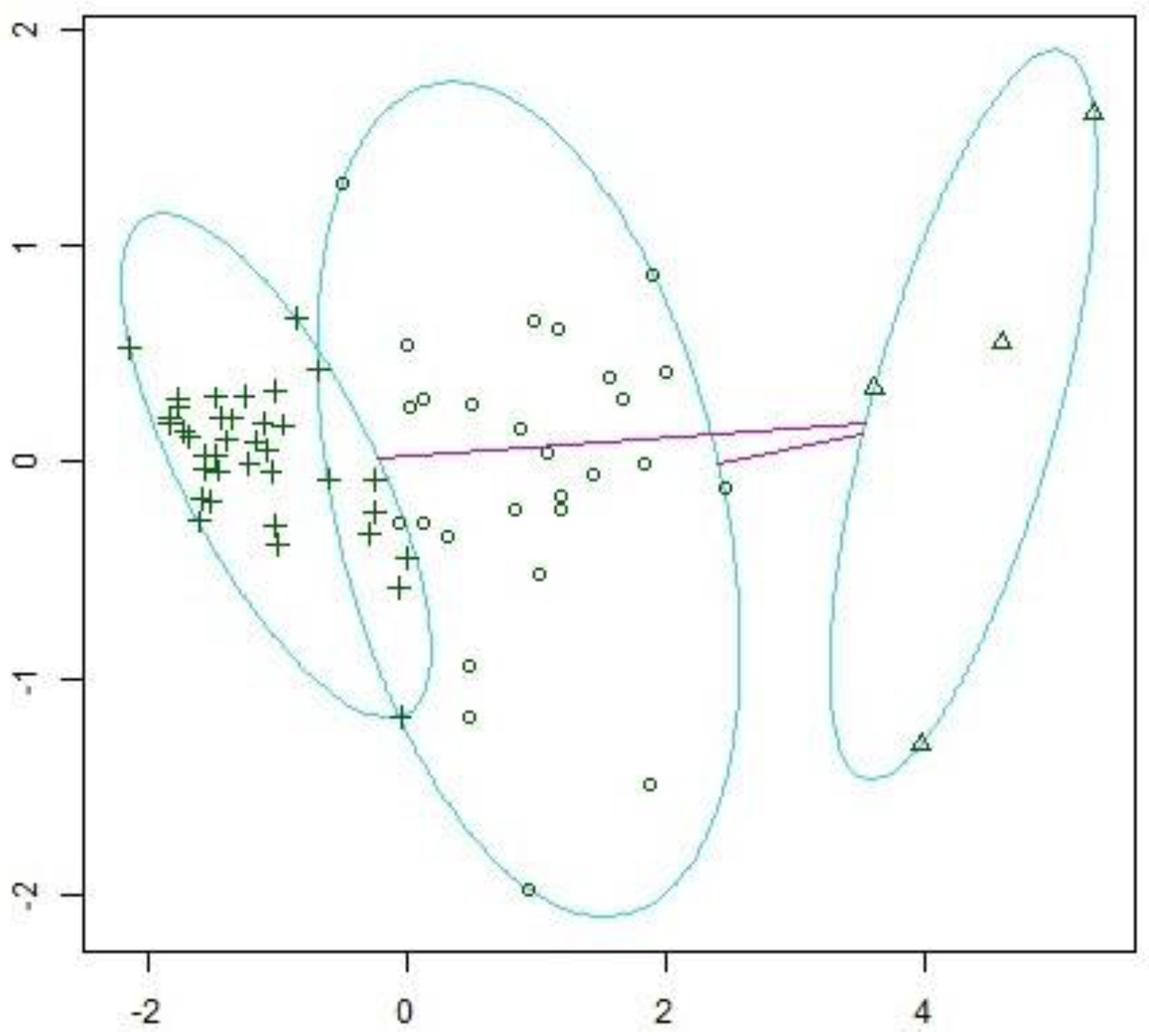
3.2. Fuzzy Modeling to Estimate Household Credit Risk

Grounded in the microdata from the household budget survey, we propose fuzzy modeling to estimate household non-payment risk, based on the optimized equivalence scales calculated in the previous section. These optimized equivalence scales allow for an estimation of the equivalent income quartile according to the region (autonomous community) of residence. The following three variables are additionally considered: arrears on mortgage or rent payments; arrears on utility bills; and arrears on hire purchase installments or other loan payments. With this set of variables, a fuzzy clustering of the data into three clusters (high, medium, and low) is proposed. The metric used for calculating dissimilarities between observations is the squared Euclidean distance.

In Figure 1, we can visualize the three fuzzy clusters obtained. The two components explain 97.81% of the point variability. The Davies–Bouldin Index is 0.68, which can be considered good, while the Calinski–Harabasz Index is 118.17, which can be seen as quite good. In addition, the average silhouette width is 0.69, which is reasonable and close to being considered strong.

Table 5. Membership degrees (probabilities) of fuzzy risk clusters in regions.

Region	Disposable Income Quartile	Cluster 1 (High)	Cluster 2 (Medium)	Cluster 3 (Low)
Basque Country	Q1	0.76	0.18	0.06
Balearic I.	Q1	0.81	0.12	0.06
Asturias	Q1	0.06	0.89	0.05
C. Valenciana	Q2	0.03	0.70	0.27
Galicia	Q2	0.03	0.43	0.54
Castilla y León	Q2	0.03	0.24	0.73
Canary I.	Q3	0.07	0.59	0.34
C. Madrid	Q3	0.03	0.63	0.34
Cataluña	Q3	0.03	0.31	0.66
Navarra	Q4	0.02	0.06	0.92
Aragón	Q4	0.01	0.03	0.96
Extremadura	Q4	0.00	0.01	0.99

shows the membership probabilities of the different observations according to a subset of autonomous communities and income quartiles. It can be seen that households in the same income quartile may show different levels of payment arrears (high, medium, or low) depending on the autonomous community of residence. For example, households in the second income quartile in Castilla y León have a low risk of payment arrears, with a probability of 0.73. This probability is even higher than households in the third income quartile in the Community of Madrid, with a membership probability of 0.63.

Although each observation could potentially belong to several clusters according to Table 5, it is also possible to calculate the centroids associated with each of the three clusters. These centroids are presented in

Table 6. Cluster centroids based on different arrears.

	Mortgage or Rental Payments	Utility Bills	Other
Cluster 1 (High)	21.5	18.1	10.0
Cluster 2 (Medium)	11.2	6.6	5.8
Cluster 3 (Low)	3.2	1.9	2.6

.

The calculation of the membership probabilities of each element for the different fuzzy clusters obtained in Table 5 provides an estimate of the probability of default (PD) of an obligation or debt incurred. The PD is a necessary component in credit risk models and serves to estimate potential losses (Li 2016). This variable, combined with the exposure at default (EAD) and the loss given default (LGD), allows companies to quickly estimate the expected loss (EL) for a credit exposure (Takawira and Mwamba 2022), just by multiplying the three previous terms.

An example that could illustrate the application of the research developed throughout this section is as follows: a household in Catalonia that applies for a loan to purchase a car, with an equivalent income per person in the third income quartile (i.e., between EUR 20,290 and EUR 28,994), would have a default probability of 3.8%. Then, assuming a requested loan of EUR 25,000, with a loss in case of default due to non-payment of EUR 30,000 (including interest), and a loss given default of 30%, the expected loss for credit risk would amount to the sum of EUR 342. However, the same loan under the same conditions for a household in the same equivalent income quartile but located in the Canary Islands would have a default probability of 5.8%, resulting in an expected loss for credit exposure of EUR 645.84. This amount is 52.6% higher than in Catalonia, despite the income quartile per person being the same in both autonomous communities.

4. Conclusions and Future Work

This study investigates the extension of a fuzzy non-payment risk management model based on optimized household consumption units. In order to achieve this goal, an improved estimation of these consumption units is obtained, and then, after applying fuzzy clustering, acceptable debt levels are identified, allowing for an estimation of the expected loss for a credit exposure. In this way, a mathematical model is developed based on empirical data, which allows the application of fuzzy set theory to business decision-making.

In this research, it can be seen that optimized household equivalence can be calculated through empirical observations, improving the current model that has kept these scales unchanged for three decades despite the significant and complex transformation in household composition during this period. The results of this study show an increase in equivalent consumption units derived from adults over 65 years old, from 0.19 in 2008 to 0.42 in 2023. Similarly, children under 14 years old have also increased their equivalent consumption units, from 0.21 to 0.31. With regard to the coefficient α₄ on the household economy scale, the values are generally around 0.90, except in the year 2020, when they decreased to 0.85, probably due to the impact of the COVID-19 pandemic (Jakubik and Teleu 2025) on household consumption patterns.

The consumption units thus calculated offer the interesting property of being able to estimate the total monetary consumption of an economy, through the direct multiplication of the consumption units and the average expenditure of single-person households. The relationship between these three economic magnitudes also facilitates an estimation of any of them, for example, through ratio estimators (Tiwari et al. 2022), in addition to forming the basis for the construction of nowcasting (Stundziene et al. 2024) indicators of these aggregates based on the use of time series.

In addition, the application of fuzzy clustering facilitates the classification of observations into three clusters based on their default risk, which is set as high, medium, and low for the purposes of this research. It is important to point out that households show different membership degrees depending on the region in which they are located. This is a fact that could be influenced by the significant differences in household expenditures existing in the autonomous communities, as well as the purchasing power parity (Majumder and Ray 2020) levels that vary significantly between regions. The levels of housing prices (Brzezicka 2021), which can be statistically assessed through the average price per square meter built, constitute another variable that could explain these differences. Since the EU-SILC is compiled and produced annually, the model proposed in this paper can be continuously updated on a yearly basis, and therefore it can be applied without becoming obsolete over time.

Notwithstanding the improvements achieved in this study, there are a number of opportunities that can also be considered for future research work. One of them is related to the equivalence scales, since the division proposed by the OECD between children up to 13 years old and adults 14 years and older is questionable when estimating their equivalent monetary income or consumption. As an alternative, this situation could be mitigated by adapting the main adult group to include only people between 18 and 64 years old. This age group harmonization would facilitate the interpretation of results from an economic perspective, allowing for better characterization among young people, adults, and seniors. Another possibility could be to align this group with the labor force survey, which considers individuals aged 15 and over. A potential problem that may arise is regional bias resulting from cluster analysis, which could be mitigated by incorporating regional purchasing power parities when adjusting the equivalized income.

Moreover, modeling income (Saulo et al. 2023) could also be applied to nowcast and forecast the evolution of these critical variables, providing valuable insights into their future trends and enabling more informed decision-making processes, and through this providing better estimations. Moreover, based on the estimated probabilities of each element belonging to the different fuzzy clusters in Table 5, we could opt for a more complex model by posing a decision problem (Bacci and Chiandotto 2019) and calculating the risk associated with each element based on a loss function L(X,Θ) to be defined by each decision maker.

The refined model proposed in this paper can be implemented by credit risk companies in their decision-making process. However, the results obtained should be interpreted cautiously and should always be supported by expert analysis of causality and correlation, for which fuzzy risk analysis systems facilitate the incorporation (Ignatius et al. 2018). It is also noteworthy that this model could be used directly by public administrations or non-governmental organizations to help the most vulnerable households with direct credit support measures. In this sense, some researchers have highlighted the importance that policymakers should bring to lowering household debt relative to disposable income (Piao et al. 2023).

All these findings provide new insights to continue a research line that promotes the application of fuzzy set theory, fostering a more profound comprehension of how fuzzy logic and decision-making models can address specific issues and challenges in the business sector.

References

1. Alonso Moral, Jose Maria, Ciro Castiello, Luis Magdalena, and Corrado Mencar. 2021. Explainable Fuzzy Systems: Paving the Way from Interpretable Fuzzy Systems to Explainable AI Systems. Studies in Computational Intelligence. Cham: Springer International Publishing, vol. 970. [Google Scholar] [CrossRef]
2. Ampountolas, Apostolos, Titus Nyarko Nde, Paresh Date, and Corina Constantinescu. 2021. A Machine Learning Approach for Micro-Credit Scoring. Risks 9: 50. [Google Scholar] [CrossRef]
3. Bacci, Silvia, and Bruno Chiandotto. 2019. Introduction to Statistical Decision Theory: Utility Theory and Causal Analysis. New York: Chapman and Hall/CRC. [Google Scholar] [CrossRef]
4. Bahoo, Salman, Marco Cucculelli, Xhoana Goga, and Jasmine Mondolo. 2024. Artificial Intelligence in Finance: A Comprehensive Review through Bibliometric and Content Analysis. SN Business & Economics 4: 23. [Google Scholar] [CrossRef]
5. Balestra, Carlotta, and Friderike Oehler. 2023. Measuring the Joint Distribution of Household Income, Consumption and Wealth at the Micro-Level: Methodological Issues and Experimental Results: 2023 Edition. Luxembourg: Publications Office of the European Union. [Google Scholar]
6. Baser, Furkan, Oguz Koc, and Ayşe Sevtap Selcuk-Kestel. 2023. Credit Risk Evaluation Using Clustering Based Fuzzy Classification Method. Expert Systems with Applications 223: 119882. [Google Scholar] [CrossRef]
7. Băban, Marius, and Călin Florin Băban. 2025. Patterns of Open Innovation Between Industry and University: A Fuzzy Cluster Analysis Based on the Antecedents of Their Collaboration. Mathematics 13: 772. [Google Scholar] [CrossRef]
8. Beck, Amir. 2023. Introduction to Nonlinear Optimization: Theory, Algorithms, and Applications with Python and MATLAB, 2nd ed. Philadelphia: Society for Industrial and Applied Mathematics. [Google Scholar] [CrossRef]
9. Bermudez Vera, Ivan Mauricio, Jaime Mosquera Restrepo, and Diego Fernando Manotas-Duque. 2025. Data Mining for the Adjustment of Credit Scoring Models in Solidarity Economy Entities: A Methodology for Addressing Class Imbalances. Risks 13: 20. [Google Scholar] [CrossRef]
10. Besharov, Douglas J., and Kenneth A. Couch. 2012. Counting the Poor: New Thinking about European Poverty Measures and Lessons for the United States. Oxford and New York: Oxford University Press. [Google Scholar]
11. Bessis, Joël. 2015. Risk Management in Banking, 4th ed. ProQuest Ebook Central. Chichester: Wiley. ISBN 978-1-118-66021-8. [Google Scholar]
12. Brown, Paul O., Meng Ching Chiang, Shiqing Guo, Yingzi Jin, Carson K. Leung, Evan L. Murray, Adam G. M. Pazdor, and Alfredo Cuzzocrea. 2022. Mahalanobis Distance Based K-Means Clustering. In Big Data Analytics and Knowledge Discovery. Edited by Robert Wrembel, Johann Gamper, Gabriele Kotsis, A. Min Tjoa and Ismail Khalil. Cham: Springer International Publishing, pp. 256–62. [Google Scholar] [CrossRef]
13. Brygała, Magdalena. 2022. Consumer Bankruptcy Prediction Using Balanced and Imbalanced Data. Risks 10: 24. [Google Scholar] [CrossRef]
14. Brzezicka, Justyna. 2021. Towards a Typology of Housing Price Bubbles: A Literature Review. Housing, Theory and Society 38: 320–42. [Google Scholar] [CrossRef]
15. Chang, Victor, Sharuga Sivakulasingam, Hai Wang, Siu Tung Wong, Meghana Ashok Ganatra, and Jiabin Luo. 2024. Credit Risk Prediction Using Machine Learning and Deep Learning: A Study on Credit Card Customers. Risks 12: 174. [Google Scholar] [CrossRef]
16. Chen, Ning, Bernardete Ribeiro, and An Chen. 2016. Financial Credit Risk Assessment: A Recent Review. Artificial Intelligence Review 45: 1–23. [Google Scholar] [CrossRef]
17. Černevičienė, Jurgita, and Audrius Kabašinskas. 2024. Explainable Artificial Intelligence (XAI) in Finance: A Systematic Literature Review. Artificial Intelligence Review 57: 216. [Google Scholar] [CrossRef]
18. Eiselt, H. A., and Carl-Louis Sandblom, eds. 2019. Methods for Nonlinearly Constrained Problems. In Nonlinear Optimization. Cham: Springer International Publishing, vol. 282, pp. 243–78. [Google Scholar] [CrossRef]
19. Eurostat. 2020. The Comparability of the EU-SILC Income Variable: Reviews and Recommendations: 2020 Edition. Luxembourg: Publications Office of the European Union. [Google Scholar]
20. Eurostat. 2022. Improving the Measurement of Poverty and Social Exclusion in Europe: Reducing Non Sampling Errors: 2022 Edition. Luxembourg: Publications Office of the European Union. [Google Scholar]
21. Ferraro, Maria Brigida. 2024. Fuzzy k-Means: History and Applications. Econometrics and Statistics 30: 110–23. [Google Scholar] [CrossRef]
22. Ferraro, Maria Brigida, Paolo Giordani, and Alessio Serafini. 2019. Fclust: An R Package for Fuzzy Clustering. The R Journal 11: 198. [Google Scholar] [CrossRef]
23. Fisher, Jonathan D. 2019. Who Files for Personal Bankruptcy in the United States? Journal of Consumer Affairs 53: 2003–26. [Google Scholar] [CrossRef]
24. Fritz-Morgenthal, Sebastian, Bernhard Hein, and Jochen Papenbrock. 2022. Financial Risk Management and Explainable, Trustworthy, Responsible AI. Frontiers in Artificial Intelligence 5: 779799. [Google Scholar] [CrossRef]
25. Hashemi, Seyed Hossein, Seyed Ali Mousavi Dehghani, Seyed Ehsan Samimi, Mahmood Dinmohammad, and Seyed Abdolrasoul Hashemi. 2020. Performance Comparison of GRG Algorithm with Evolutionary Algorithms in an Aqueous Electrolyte System. Modeling Earth Systems and Environment 6: 2103–10. [Google Scholar] [CrossRef]
26. Ignatius, Joshua, Adel Hatami-Marbini, Amirah Rahman, Lalitha Dhamotharan, and Pegah Khoshnevis. 2018. A Fuzzy Decision Support System for Credit Scoring. Neural Computing and Applications 29: 921–37. [Google Scholar] [CrossRef]
27. Izquierdo Llanes, Gregorio, and Antonio Salcedo. 2023. Why Does Equivalization Matter? An Application to the Monetary Poverty in the Sustainable Development Goals Framework. Quality & Quantity 57: 2575–89. [Google Scholar] [CrossRef]
28. Jahn, Johannes. 2020. Introduction to the Theory of Nonlinear Optimization. Cham: Springer International Publishing. [Google Scholar] [CrossRef]
29. Jakubik, Petr, and Saida Teleu. 2025. Improving Credit Risk Assessment in Uncertain Times: Insights from IFRS 9. Risks 13: 38. [Google Scholar] [CrossRef]
30. Kerre, Etienne, and John Mordeson. 2018. Fuzzy Mathematics. Basel: MDPI. [Google Scholar] [CrossRef]
31. Leland, Hayne E. 2012. Predictions of Default Probabilities in Structural Models of Debt. In The Credit Market Handbook, 1st ed. Edited by H. Gifford Fong. Hoboken: Wiley, pp. 39–64. [Google Scholar] [CrossRef]
32. Li, Weiping. 2016. Probability of Default and Default Correlations. Journal of Risk and Financial Management 9: 7. [Google Scholar] [CrossRef]
33. Majumder, Amita, and Ranjan Ray. 2020. National and Subnational Purchasing Power Parity: A Review. Decision 47: 103–24. [Google Scholar] [CrossRef]
34. Mazzini, Gabriele, and Filippo Bagni. 2023. Considerations on the Regulation of AI Systems in the Financial Sector by the AI Act. Frontiers in Artificial Intelligence 6: 1277544. [Google Scholar] [CrossRef] [PubMed]
35. Milana, Carlo, and Arvind Ashta. 2021. Artificial Intelligence Techniques in Finance and Financial Markets: A Survey of the Literature. Strategic Change 30: 189–209. [Google Scholar] [CrossRef]
36. Mussabayev, Rustam. 2024. Optimizing Euclidean Distance Computation. Mathematics 12: 3787. [Google Scholar] [CrossRef]
37. Nahar, Janifer, Md Atiqur Rahaman, Md Alauddin, and Farhana Zaman Rozony. 2024. Big Data in Credit Risk Management: A Systematic Review of Transformative Practices and Future Directions. International Journal of Management Information Systems and Data Science 1: 68–79. [Google Scholar] [CrossRef]
38. Nkambule, Dumisani Selby, Bhekisipho Twala, and Jan Harm Christiaan Pretorius. 2024. Effective Machine Learning Techniques for Dealing with Poor Credit Data. Risks 12: 172. [Google Scholar] [CrossRef]
39. OECD. 2013. OECD Framework for Statistics on the Distribution of Household Income, Consumption and Wealth. Paris: OECD. [Google Scholar] [CrossRef]
40. Piao, Ying’ai, Meiru Li, Hongyuan Sun, and Ying Yang. 2023. Income Inequality, Household Debt, and Consumption Growth in the United States. Sustainability 15: 3910. [Google Scholar] [CrossRef]
41. Salazar, Fabian Leandro Moreno, and Juan Carlos Figueroa-García. 2025. Fuzzy Theory in Credit Scoring: A Literature Review. In Advanced Research in Technologies, Information, Innovation and Sustainability. Edited by Teresa Guarda, Filipe Portela and Maria Fernanda Augusto. Cham: Springer Nature Switzerland, vol. 2348, pp. 55–68. [Google Scholar] [CrossRef]
42. Sanchez-Roger, Marc, María Dolores Oliver-Alfonso, and Carlos Sanchís-Pedregosa. 2019. Fuzzy Logic and Its Uses in Finance: A Systematic Review Exploring Its Potential to Deal with Banking Crises. Mathematics 7: 1091. [Google Scholar] [CrossRef]
43. Saulo, Helton, Roberto Vila, Giovanna V. Borges, Marcelo Bourguignon, Víctor Leiva, and Carolina Marchant. 2023. Modeling Income Data via New Parametric Quantile Regressions: Formulation, Computational Statistics, and Application. Mathematics 11: 448. [Google Scholar] [CrossRef]
44. Sisodia, Bhupendra Veer Singh, and Dhirendra Singh. 2020. Calibration Approach-Based Estimators for Finite Population Mean in Multistage Stratified Random Sampling. In Statistical Methods and Applications in Forestry and Environmental Sciences. Edited by Girish Chandra, Raman Nautiyal and Hukum Chandra. Singapore: Springer, pp. 105–23. [Google Scholar] [CrossRef]
45. Stundziene, Alina, Vaida Pilinkiene, Jurgita Bruneckiene, Andrius Grybauskas, Mantas Lukauskas, and Irena Pekarskiene. 2024. Future Directions in Nowcasting Economic Activity: A Systematic Literature Review. Journal of Economic Surveys 38: 1199–1233. [Google Scholar] [CrossRef]
46. Takawira, Oliver, and John W. Muteba Mwamba. 2022. Sovereign Credit Ratings Analysis Using the Logistic Regression Model. Risks 10: 70. [Google Scholar] [CrossRef]
47. Tiwari, Kuldeep Kumar, Sandeep Bhougal, and Sunil Kumar. 2022. A Comparative Study of Ratio Estimators with Regression Estimator. Journal of Statistics Applications & Probability Letters 9: 101–4. [Google Scholar] [CrossRef]
48. UNECE. 2017. Guide on Poverty Measurement. e-ISBN: 9789213627907. Available online: https://digitallibrary.un.org/record/3931399/files/ECECESSTAT20174.pdf (accessed on 4 February 2025).
49. Vagaská, Alena, and Miroslav Gombár. 2021. Mathematical Optimization and Application of Nonlinear Programming. In Algorithms as a Basis of Modern Applied Mathematics. Edited by Šárka Hošková-Mayerová, Cristina Flaut and Fabrizio Maturo. Cham: Springer International Publishing, pp. 461–86. [Google Scholar] [CrossRef]
50. Wang, Hao, Anthony Bellotti, Rong Qu, and Ruibin Bai. 2024. Discrete-Time Survival Models with Neural Networks for Age–Period–Cohort Analysis of Credit Risk. Risks 12: 31. [Google Scholar] [CrossRef]
51. Wang, Xingqi, and Zhenhua Mao. 2023. Research on the Impact of Digital Inclusive Finance on the Financial Vulnerability of Aging Families. Risks 11: 209. [Google Scholar] [CrossRef]
52. Weber, Patrick, K. Valerie Carl, and Oliver Hinz. 2024. Applications of Explainable Artificial Intelligence in Finance—A Systematic Review of Finance, Information Systems, and Computer Science Literature. Management Review Quarterly 74: 867–907. [Google Scholar] [CrossRef]
53. Wilhelmina Afua Addy, Chinonye Esther Ugochukwu, Adedoyin Tolulope Oyewole, Onyeka Chrisanctus Ofodile, Omotayo Bukola Adeoye, and Chinwe Chinazo Okoye. 2024. Predictive Analytics in Credit Risk Management for Banks: A Comprehensive Review. GSC Advanced Research and Reviews 18: 434–49. [Google Scholar] [CrossRef]
54. Wójcicka-Wójtowicz, Aleksandra, and Krzysztof Piasecki. 2021. Application of the Oriented Fuzzy Numbers in Credit Risk Assessment. Mathematics 9: 535. [Google Scholar] [CrossRef]
55. Zhang, Shixiao, Peisong Han, and Changbao Wu. 2023. Calibration Techniques Encompassing Survey Sampling, Missing Data Analysis and Causal Inference. International Statistical Review 91: 165–92. [Google Scholar] [CrossRef]
56. Zhao, Xianbo, Bon-Gang Hwang, and Sui Pheng Low. 2015. Risk Management and Enterprise Risk Management. In Enterprise Risk Management in International Construction Operations. Edited by Xianbo Zhao, Bon-Gang Hwang and Sui Pheng Low. Singapore: Springer, pp. 33–83. [Google Scholar] [CrossRef]
Figure 1. Cluster visualization of the dataset.
Risks 13 00074 g001