Operational Choices for Risk Aggregation in Insurance: PSDization and SCR Sensitivity

Abstract

This work addresses crucial questions about the robustness of the PSDization process for applications in insurance. PSDization refers to the process that forces a matrix to become positive semidefinite. For companies using copulas to aggregate risks in their internal model, PSDization occurs when working with correlation matrices to compute the Solvency Capital Requirement (SCR). We examine how classical operational choices concerning the modelling of risk dependence impacts the SCR during PSDization. These operations refer to the permutations of risks (or business lines) in the correlation matrix, the addition of a new risk, and the introduction of confidence weights given to the correlation coefficients. The use of genetic algorithms shows that theoretically neutral transformations of the correlation matrix can surprisingly lead to significant sensitivities of the SCR (up to 6%). This highlights the need for a very strong internal control around the PSDization step.

1. Introduction

When measuring the insurer’s exposure to numerous risks, and especially to assess their own funds requirement (or Solvency Capital Requirement in insurance, denoted further by SCR, and representing the 99.5th percentile of the aggregated loss distribution), one of the most sensitive steps is the modelling of the dependence between those risks.

This is of course a major question, which, as such, has recently attracted attention from the scientific community. See, for instance, the works by Georgescu et al. (2017), Cifuentes and Charlin (2016), Bernard et al. (2014), Clemente and Savelli (2013), Cheung and Vanduffel (2013), Clemente and Savelli (2011), Devineau and Loisel (2009), Filipovic (2009), Sandström (2007), Denuit et al. (1999), and references therein. This aggregation step allows for taking into account mitigation, or the potentiality of those individual risks occurring simultaneously. According to the European Directive Solvency II (EIOPA (2009)), there are two main approaches to compute aggregated risk measures considering the dependence structure between risks. In the first case, this aggregation is performed through a variance–covariance approach via the Standard Formula, below

$$SCR=\sqrt{\sum _{i\in 〚1,n〛}\sum _{j\in 〚1,n〛}{\rho }_{ij}\times SC{R}_i\times SC{R}_j},$$

(1)

where $SC{R}_i$ is the 99.5th percentile of the random loss $X_i$ associated to risk i, and ${\rho }_{ij}$ is the linear correlation such that ${\rho }_{ij}=Cov(X_i,X_j)/\sqrt{Var\left(X_i\right)Var\left(X_j\right)}$. This technique was shown to be valid for elliptical loss distributions, which is not the case in general1.

Another possibility for insurers is to calculate the SCR thanks to their internal model, once the latter has been approved by supervisors. In this case, insurers usually work with copulas for the aggregation of risk factors in order to obtain the full distribution of losses. Copulas can indeed model most general situations of dependence, as shown by the well known Sklar’s theorem. In practice, internal models require the implementation of these successive steps:

• calibration of marginal distributions for each risk factor (e.g., equity, interest rates);
• modelling the dependence between risk factors through a copula;
• aggregation of risks, leading to the entire distribution of the aggregate loss (sometimes an intermediate step links the risk factors to their associated loss thanks to proxy functions, see Section 5.1). Taking the 99.5th percentile of this distribution allows the evaluation of the SCR.

The aggregation thus requires a correlation matrix as an input, whatever the technique (at least when copulas are Gaussian or Student, which is the case for several insurance companies using an internal model). The dimensions of this matrix can be huge in practice (e.g., 1000 × 1000, i.e., with around 500,000 different values), depending on the modular structure chosen (for instance, the dimensions of correlation matrices remain low in the Standard Formula, see Section 2.1). The matrix includes numerous correlation coefficients that can result from empirical statistical measures, expert judgments or automatic formulas. As a matter of fact, it is thus rarely2 positive semidefinite (PSD): this is what is commonly called a pseudo-correlation matrix. Unfortunately, this matrix cannot be used directly to aggregate risks. Indeed, both variance–covariance and copula aggregation techniques require the correlation matrix to be PSD (that is with all eigenvalues $\ge 0$) for the following main reasons:

• Coherence: it is a well-known property that correlation matrices are PSD. Negative eigenvalues indicate that a logical error was made while establishing the coefficients of the matrix. For instance, consider the case of a 3 × 3 matrix: if the coefficients indicate a strong positive correlation between the first and second risk factors, a strong positive correlation between the second and third risk factors, but a strong negative correlation between the first and third risk factors, this will generate a negative eigenvalue corresponding to the coherence mistake made.
• Prudence: taking more risk could decrease the insurer’s SCR if there exists one negative eigenvalue associated to an eigenvector with positive coefficients. For instance, consider the loss vector (100 M€, 10 M€, 40 M€) and the correlation matrix

  $$\rho =\left(\begin{array}{ccc}{\rho }_{11}& {\rho }_{12}& {\rho }_{13}\\ {\rho }_{21}& {\rho }_{22}& {\rho }_{23}\\ {\rho }_{31}& {\rho }_{32}& {\rho }_{33}\end{array}\right)=\left(\begin{array}{ccc}1& -0.9& -0.5\\ -0.9& 1& -0.5\\ -0.5& -0.5& 1\end{array}\right).$$
  Using the variance–covariance approach, the riskiest situation in terms of losses (106.20 M€; 16.20 M€; 44.81 M€) leads to a lower SCR (70.48 M€ against 74.16 M€).
• Ability to perform simulations: in the copula approach, the input correlation matrix has to be PSD to apply Choleski decomposition. This is necessary for Gaussian or Student vectors, which are the most common cases for such tasks in practice.

Using PSD correlation matrices is therefore crucial, which explains why it is explicitly required by the Delegated Rules of the Solvency II regulation (EIOPA (2015), see Appendix XVIII). Accordingly, insurers apply algorithms on their pseudo-correlation matrix in order to make it become PSD: this is the so-called PSDization process. Most common algorithms can be separated into three categories: Alternating Projections, Newton and Hypersphere algorithms. One focuses in this paper on the Rebonato–Jäckel algorithm, which belongs to the latter family (see Section 3 for further details about the motivation of this choice).

Considering this framework, the impact on the SCR of standard operations on the correlation matrix should be verified. Our interest lies in studying operational choices such as weighting the correlation coefficients during PSDization (to reflect the confidence experts may have on these coefficients), switching some columns of the matrix (i.e., reordering the risks before aggregation), or adding one dimension (which can correspond to an additional business line with low materiality on the overall SCR). To the authors’ knowledge, the impact of such operations on the PSDization step has not been studied formally in the literature before. Numerical examples support the main idea of this work: transformations of the matrix, with low or null theoretical impact on the SCR, sometimes lead to unexpected changes of this global SCR. For large insurance companies, this is all the more important since a 1% change of SCR can cost millions of euros in terms of capital. This would strongly affect the Return On Equity index, an essential profitability indicator for investors.

The publication is organized as follows: Section 2 introduces the pseudo-correlation matrices to be considered hereafter. Section 3 describes most common PSD algorithms, and motivates our choice. With the help of some significant examples, Section 4 illustrates to which extent PSDization leads to modifying the initial pseudo-correlation coefficients. The cases of higher risk matrix dimensions, weighted correlation coefficients and risk permutations are studied. Finally, real-life sensitivities are assessed in Section 5 thanks to the use of genetic algorithms and simulations, and provide some interesting results concerning the aforementioned operations and their impact on the global SCR of the company.

2. Pseudo-Correlation Matrices under Study

2.1. Correlation Matrices of the Standard Formula

Before studying the algorithms which enable a matrix to be PSD when using an internal model, one must check that the matrices defined by the standard formula are already PSD. As a reminder, the Standard Formula given by the regulation states that risks should be aggregated in a bottom-up approach, with a tree-based structure. This means that individual SCRs first have to be assessed, each one corresponding to a module (Life, Non Life, and so on). Solvency II texts then define several correlation matrices for each level of aggregation.

Table 1. Eigenvalues of correlation matrices in Solvency II regulation (the matrices are available in EIOPA (2015), with further details concerning the corresponding article or appendix in the table).

Module	Dimension	${\mathit{\lambda }}_1$	${\mathit{\lambda }}_2$	${\mathit{\lambda }}_3$	${\mathit{\lambda }}_4$	${\mathit{\lambda }}_5$	${\mathit{\lambda }}_6$	${\mathit{\lambda }}_7$	${\mathit{\lambda }}_8$	${\mathit{\lambda }}_9$	${\mathit{\lambda }}_{10}$	${\mathit{\lambda }}_{11}$	${\mathit{\lambda }}_{12}$	PSD
Global (App. IV)	5	1.92	1.16	0.75	0.75	0.40								Yes
Market up (Art. 164)	6	2.47	1.18	1.00	0.68	0.50	0.15							Yes
Market down (Art. 164)	6	2.89	1.00	0.87	0.57	0.50	0.15							Yes
Life (Art. 136)	7	2.18	1.51	1.07	0.81	0.70	0.57	0.12						Yes
Health SLT (Art. 151)	6	2.04	1.43	1.00	0.81	0.58	0.12							Yes
Health non SLT (App. XV)	4	3	0.5	0.5	0.5									Yes
Health (Art. 144)	3	1.68	0.81	0.5										Yes
Non Life (Art. 114)	3	1.25	1	0.75										Yes
Prem. Reserve (App. IV)	12	4.91	1.45	1.09	0.97	0.73	0.68	0.61	0.48	0.38	0.33	0.20	0.12	Yes

shows that the eigenvalues of these matrices are all positive, meaning that they are PSD. Except for the global matrix that can be found in the Directive, all matrices are described in the Delegated Acts (see references in the first column of Table 1).

2.2. Notations and Correlation Matrices under Study

Throughout the paper, $G_{xy}$ indicates the initial pseudo-correlation matrix to be PSDized, where x refers to the matrix dimension and y is the number of the example. When using weights to apply to the correlation coefficients during PSDization, a weighting matrix $H_{xy}$ is defined. Then, we denote by $S_{xy}^{PA}$ the PSDized matrix obtained from $G_{xy}$ using the Alternated Projections algorithm; $S_{xy}^N$ the PSDized matrix with the Newton algorithm; $S_{xy}$ the PSDized matrix with the Hypersphere algorithm and $S_{xy}^H$ the PSDized matrix with the Hypersphere algorithm using a weighting matrix H. The use of a weighting matrix enables the adjustment in terms of importance of one or several correlation coefficients with respect to other coefficients when making the correlation matrix PSD. This is very useful for insurance companies, since some coefficients can have a bigger impact on the final capital requirement, and the aim would be that PSDization modifies these coefficients as little as possible. It must be noted that some algorithms (Newton, Hypersphere) can be extended to use constraints on the correlation coefficients, such as ${\rho }_{ij}^{min}\le {\rho }_{ij}\le {\rho }_{ij}^{max}$. However, these extensions are left for future research for two main reasons: very few practitioners use them, and they cause non-trivial theoretical and practical issues (there could be no solution, i.e., PSDized matrix, according to the constrained set).

Our examples are built with the same simple idea: assess the impact of PSDization combined to classical operational choices on various situations to reflect the real world. We thus consider correlation matrices of various dimensions, with positive and negative eigenvalues, and with a high heterogeneity regarding their individual correlation coefficients (positive, negative, far or close to extreme values −1 or +1). The seven examples studied all along the paper are listed in Appendix A, including the 10-dimension correlation matrix that has been created manually. This example was designed with the aim of having a certain coherence with the reality of risk aggregation in insurance. The first risk factor, say $X_1$, refers to the risk that interest rates decrease ($X_2$ represents the risk of interest rates increasing). $X_3$ corresponds to unexpected high expenses, $X_4$ relates to the incorrect assessment of the level of expenses, and $X_5$ is the risk of spreads increasing. The risk that market stocks drop is given by $X_6$, $X_7$ accounts for the longevity risk, $X_8$ is the mass lapse risk, $X_9$ corresponds to the underwriting risk (premium and reserve risk as in the standard formula, see (CEIOPS 2010, p. 118), which could also be modelled by two different risk factors in internal models) in the Health business line; and $X_{10}$ is the underwriting risk in short-term disability.

Correlation coefficients were determined either by statistical measures built on historical data on financial markets, or by expert opinions. To read the matrix appropriately, the linear correlation between $X_1$ and $X_2$ is the coefficient ${\rho }_{12}$ (or ${\rho }_{21}$), located on line 1 column 2 (of course, the coefficient equals $-1$ in this case). Finally, our pseudo-correlation matrix looks like

$$G_{101}=\left(\begin{array}{cccccccccc}1& -1& -0.28& 0& 0.63& -0.47& 0.25& 0.75& 0& 0\\ -1& 1& 0.77& 0.5& -0.38& 0.88& 0.25& 0.75& 0.25& 0.25\\ -0.28& 0.77& 1& 0.25& 0.25& 0.17& -0.25& 0.25& 0.5& 0.5\\ 0& 0.5& 0.25& 1& 0.25& 0.25& 0& 0.5& 0.5& 0.5\\ 0.63& -0.38& 0.25& 0.25& 1& 0.83& 0.25& 0.75& 0& 0\\ -0.47& 0.88& 0.17& 0.25& 0.83& 1& 0.75& 0.75& 0& 0\\ 0.25& 0.25& -0.25& 0& 0.25& 0.75& 1& 0.5& 0.25& 0.25\\ 0.75& 0.75& 0.25& 0.5& 0.75& 0.75& 0.5& 1& 0.25& 0.25\\ 0& 0.25& 0.5& 0.5& 0& 0& 0.25& 0.25& 1& 0.75\\ 0& 0.25& 0.5& 0.5& 0& 0& 0.25& 0.25& 0.75& 1\end{array}\right).$$

Table 2. Eigenvalues in our examples, before PSDization.

Example #	Dimension	Notation	${\mathit{\lambda }}_1$	${\mathit{\lambda }}_2$	${\mathit{\lambda }}_3$	${\mathit{\lambda }}_4$	${\mathit{\lambda }}_5$	${\mathit{\lambda }}_6$	${\mathit{\lambda }}_7$	${\mathit{\lambda }}_8$	${\mathit{\lambda }}_9$	${\mathit{\lambda }}_{10}$	PSD
1	3	$G_{31}$	1.90	1.39	$-0.29$								No
2	3	$G_{32}$	1.91	1.44	$-0.35$								No
3	4	$G_{41}$	2.17	1.27	0.88	$-0.32$							No
4	4	$G_{42}$	1.95	1.74	0.96	$-0.64$							No
5	5	$G_{51}$	2.80	1.98	1.16	$-0.17$	$-0.77$						No
6	5	$G_{52}$	2.44	1.97	1.67	$-0.19$	$-0.88$						No
7	10	$G_{101}$	3.93	2.72	2.00	1.14	0.74	0.57	0.25	$-0.03$	$-0.55$	$-0.77$	No

sums up the eigenvalues of our seven pseudo-correlation matrices: note that none of the considered matrices is PSD. However, some of them are not very far from having this property.

3. Selection of an Adequate Algorithm for PSDization

PSDization algorithms aim to build the nearest PSD matrix to an initial non-PSD matrix, where the notion of “nearest” is detailed in the sequel. This section briefly presents the main families of PSDization algorithms, and justifies our choice to work with the Hypersphere (or Rebonato-Jäckel) algorithm. Interesting recent works on this topic and more details can be found in (Cutajar et al. 2017).

3.1. Families of Algorithms

3.1.1. Alternating Projections

The Alternating Projections (AP) algorithm, introduced by Higham (2002), leads to the nearest correlation matrix under the W-norm, defined by

$$\forall A\in {\mathbb{R}}^{n\times n},{\parallel A\parallel }_W={\parallel W^{\frac{1}{2}}A{W}^{\frac{1}{2}}\parallel }_2,$$

where $\forall A\in {\mathbb{R}}^{n\times n},{\parallel A\parallel }_2^2={\sum }_{(i,j)\in 〚1;n{〛}^2}{a}_{ij}^2=tr\left(A{A}^T\right)$. This norm is also called the Frobenius norm, and $W\in {\mathbb{R}}^{n\times n}$ is a square matrix with positive coefficients.

The AP algorithm corresponds to a linear optimization, projecting alternately the matrix obtained at each step on two convex closed subsets of the matrix space ${\mathbb{R}}^{n\times n}$. It enables in particular to show the uniqueness of the solution under this type of norm.

However, the W-norm does not in general correspond to the norm insurers may be interested in. The H-norm, defined by $\forall A\in {\mathbb{R}}^{n\times n},{\parallel A\parallel }_H^2={\sum }_{(i,j)\in 〚1;n{〛}^2}{h}_{ij}{a}_{ij}^2$, where $H\in {\mathbb{R}}^{n\times n}$ offers more flexibility to weight coefficients according to their materiality on the SCR, or according to the confidence level one has in the coefficients. The W-norm and the H-norm only coincide when W is diagonal ($W=diag{\left(w_i\right)}_{i\in 〚1;n〛}$) and H is a rank-1 matrix ($H=\left[{\left(w_i{w}_j\right)}^{\frac{1}{2}}\right]$). Thus, the AP algorithm lacks flexibility in that it does not enable the use of another general matrix to weight freely each individual correlation coefficient.

3.1.2. Newton Algorithm

Newton algorithms with such applications were introduced by Qi and Sun (2006). They were initially designed for the traditional 2-norm, and are therefore computationally quicker than the Alternating Projections. However, their extension to the most general case (i.e., H-norm) requires optimization techniques such as the Uzawa method. Unfortunately, the Uzawa method implies optimization within optimization, and makes the overall algorithm much more time-consuming, as well as much more complex to interpret.

3.1.3. Rebonato–Jäckel Algorithm

Belonging to the family of Hypersphere algorithms, the Rebonato–Jäckel method was initially introduced in Rebonato and Jäckel (1999). Since then, it has been extensively studied in literature, and many publications have proved its efficiency in reaching a robust solution. Its wide success is due to the following theorem (see the proof in (Jäckel 2002)): any correlation matrix $\rho$ can be written as

$$\rho =B{B}^T,$$

where the coefficients of the matrix $B\in {\mathbb{R}}^{n\times n}$ can be written as:

$$\left\{\begin{array}{c}\forall (i,j)\in 〚1;n〛\times 〚1;n-1〛,B_{ij}=cos\left({\theta }_{ij}\right){\prod }_{k=1}^{j-1}sin\left({\theta }_{ik}\right),\hfill \\ \forall i\in 〚1;n〛,B_{in}={\prod }_{k=1}^{n-1}sin\left({\theta }_{ik}\right).\hfill \end{array}\right.$$

In addition, the angular vector $\theta$ is unique if:

$$\left\{\begin{array}{c}\forall (i,j)\in 〚1;n〛\times 〚1;n-1〛,{\theta }_{ij}\in [0,\pi ],\hfill \\ \forall i\le j,{\theta }_{ij}=0.\hfill \end{array}\right.$$

The Hypersphere algorithm thus consists of looking for the solution matrix under the abovementioned form. It offers several advantages; in particular, it is simple to use, easily understandable, and is the most widely used algorithm in the bank and insurance sectors. Moreover, it allows the use of the H-norm and converges fairly quickly. However, its main weakness lies in that it sometimes converges to a local minimum, and therefore does not guarantee that the output is the nearest PSDized correlation matrix. This drawback has to be kept in mind, since it may have other side effects. Let us mention for instance the fact that the order in which risk factors are considered in the correlation matrix matters, although it should not (see Section 4 and Section 5).

3.2. Choice of the Algorithm for the Rest of the Paper

To check the robustness when performing PSDization with these algorithms, one first compares the distances between the initial pseudo-correlation matrix and its PSDized version in the three different cases. Of course, the lower this distance is, the better the algorithm. We use the Frobenius-norm (see Section 3.1.1), since it is common to all algorithms.

Results about PSDized versions for each example are detailed in Appendix B: note that the PSDized correlation matrices are the same when the dimension remains low, whatever the algorithm considered. More precisely, the three algorithms give very similar results with PSDized versions of $G_{31}$, $G_{32}$, $G_{41}$, $G_{42}$, $G_{51}$, and $G_{52}$ (same coefficients, up to ${10}^{-4}$). On the contrary, the PSDized versions of $G_{101}$ are slightly different depending on the algorithm used. As an illustration, we get the following distances:

$$\left|\right|S_{101}^{PA}-G_{101}{\left|\right|}_2=\left|\right|S_{101}^N-G_{101}{\left|\right|}_2=1.211\le \left|\right|S_{101}-G_{101}{\left|\right|}_2=1.213.$$

In this example, it seems that the first two algorithms give better results. The Rebonato-Jäckel algorithm is likely to have selected a locally-optimal solution. Despite not being the best technique in this particular case, we will use the latter for three main reasons in coming analyses: (i) distances do not seem to be significantly different from one method to another; (ii) the Rebonato-Jäckel algorithm enables the easy introduction of confidence weights to the individual correlation coefficients in practice (through the H-norm), which is a key point; and (iii) the Rebonato-Jäckel algorithm is fast and easy to interpret. Indeed, experts know that some initial coefficient values can be particularly reliable, or they can anticipate that some of them will have a significant impact on the global SCR.

3.3. One PSDization Example: The 10-Dimensional Matrix

Trying to replicate the conditions in which insurers use PSDization algorithms, it is clearly more appropriate to consider the H-norm. Indeed, it makes it possible to integrate confidence weights given to correlation coefficients during the PSDization process. PSDization of $G_{101}$ using the Rebonato-Jackël algorithm and the weighting matrix $H_{101}$ (see Appendix A) leads to a new correlation matrix $S_{101}^H$ (disclosed in Appendix C), with the eigenvalues below

$$\lambda \in \{3.70;2.49;1.83;1.05;0.64;0.27;0.02;0.00;0.00;0.00\}.$$

The three last values equal ${10}^{-5}$, which is the lower bound defined in the algorithm. This means that the three negative eigenvalues of $G_{101}$ (see Table 2) have been replaced by the lowest possible value. One then measures the standardized distance between the initial pseudo-correlation matrix $G_{101}$ and its PSDized version $S_{101}^H$:

$$D_{101}^H={\displaystyle \frac{\left|\right|S_{101}^H-G_{101}{\left|\right|}_H}{\left|\right|G_{101}{\left|\right|}_H}}=19.7\%.$$

It thus seems that PSDization globally had a great impact on the pseudo-correlation matrix. Some coefficients were strongly modified, see for instance ${\rho }_{65}$ (fictional correlation between equity and spreads). Indeed, ${\rho }_{65}$ equals 0.83 at the beginning in $G_{101}$, but is close to 0.54 after PSDization in $S_{101}^H$. Such an example highlights the need for insurers to check all the modifications, in order to gain control and monitor their internal model.

4. Sensitivity of the Matrices to PSDization

In this section, we would like to illustrate how the correlation matrix can be modified when performing PSDization by the Rebonato-Jackël algorithm, with toy examples. We specifically investigate how the coefficients of $G_{31}$ (Appendix A) change during the sole PSDization, and also look at the evolution of individual correlation coefficients when considering other classical operations for practitioners: permutations of some coefficients before PSDization, change of matrix dimension (before PSDization), or weights given to the correlation coefficients during PSDization. For this purpose, we consider the following initial weighting matrix

$$H^{init}=\left(\begin{array}{ccc}1& 0.1& 0.9\\ 0.1& 1& 0.5\\ 0.9& 0.5& 1\end{array}\right).$$

These operations mainly correspond to the decisions that actuaries have to make when developing internal models for risk aggregation. Note that the impact on the capital requirement can be substantially different from the impact in terms of matrix norm, according to the respective importance of the loss marginals. This impact will be studied in Section 5.

4.1. Impact of Permutations

To study how permutations of risks defining the correlation matrix impact the standard PSDization process, we first consider the permutation $\sigma$ such as

$$\left(\begin{array}{ccc}1& 2& 3\\ \downarrow & \downarrow & \downarrow \\ 2& 3& 1\end{array}\right).$$

As a result,

Table 3. Modification of initial correlation coefficients due to permutations of risks.

Coefficient	Before PSDization	Direct PSDization	PSDization after Permutation
${\rho }_{12}$	−0.9	−0.585	−0.605
${\rho }_{13}$	−0.5	−0.473	−0.476
${\rho }_{23}$	−0.5	−0.437	−0.411

shows the obtained modifications of the correlation coefficients:

Examining the coefficients, we notice that they are significantly modified: first by the PSDization process itself, but also by the permutation of risks. This last result is surprising, since there should be no theoretical impact with this operation. However, because our algorithm presents local minima issues, the choice of the order of risk factors (arbitrarily made by the insurer) matters when performing PSDization.

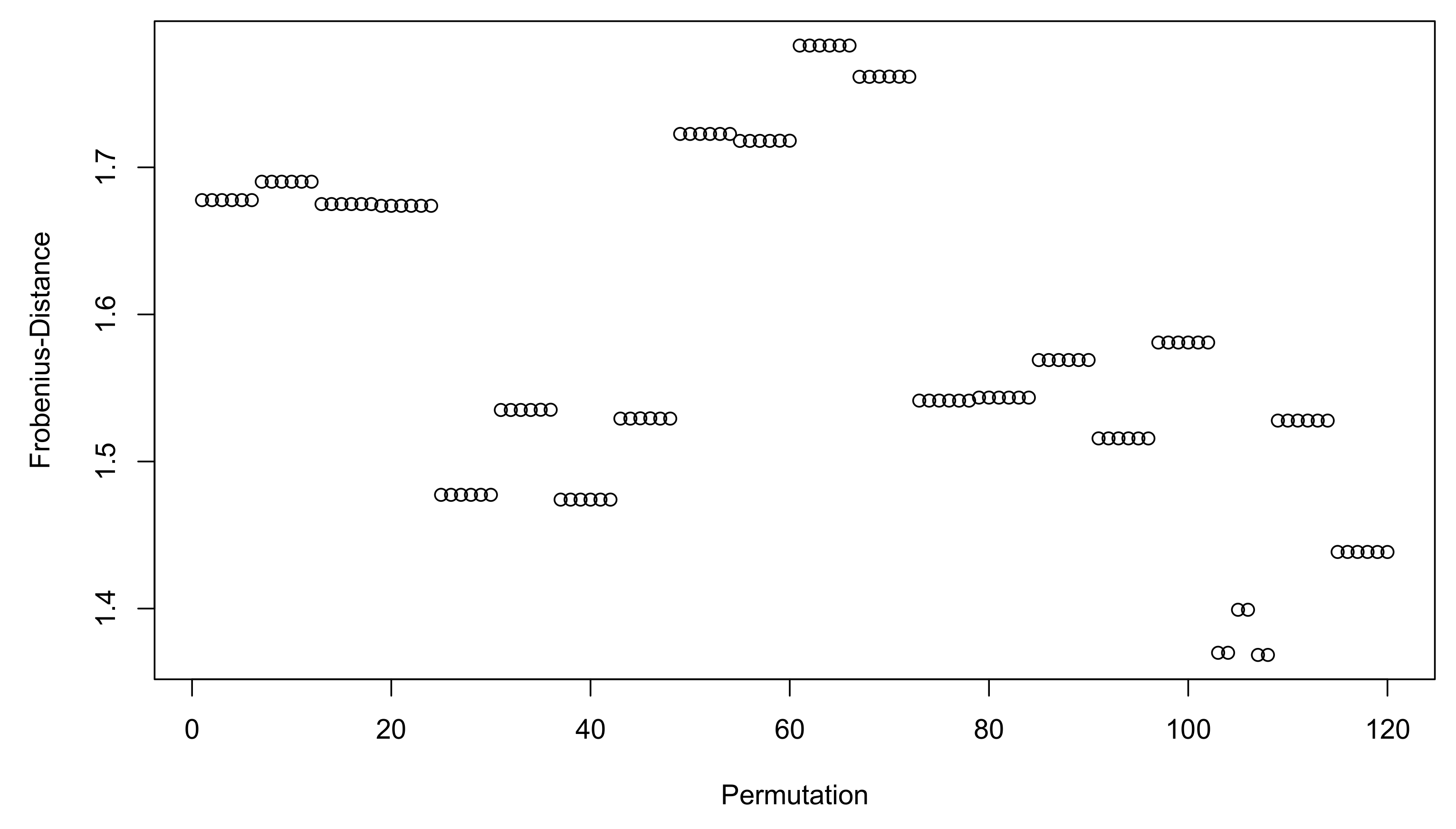
To figure out more comprehensively the impact of permutations, it would be best to look at the exhaustive list of permutations for a given pseudo-correlation matrix. Remember that a D-dimensional matrix admits D! permutations, and let us consider the example $G_{51}$. Figure 1 shows the Frobenius distance to the initial matrix for the 5! permutations of $G_{51}$, knowing that this distance between $G_{51}$ and $S_{51}^H$ initially equals 1.68 without any permutation. The Frobenius norm is clearly not the norm that the algorithm optimizes, but it simply illustrates to which extent the solution matrix $S_{51}^H$ is modified. Two remarks can be made here. First, the distances follow a block pattern caused by the order of the permutations. Second, the permutations do not always lead to an increase in the distance to the initial pseudo-correlation matrix.

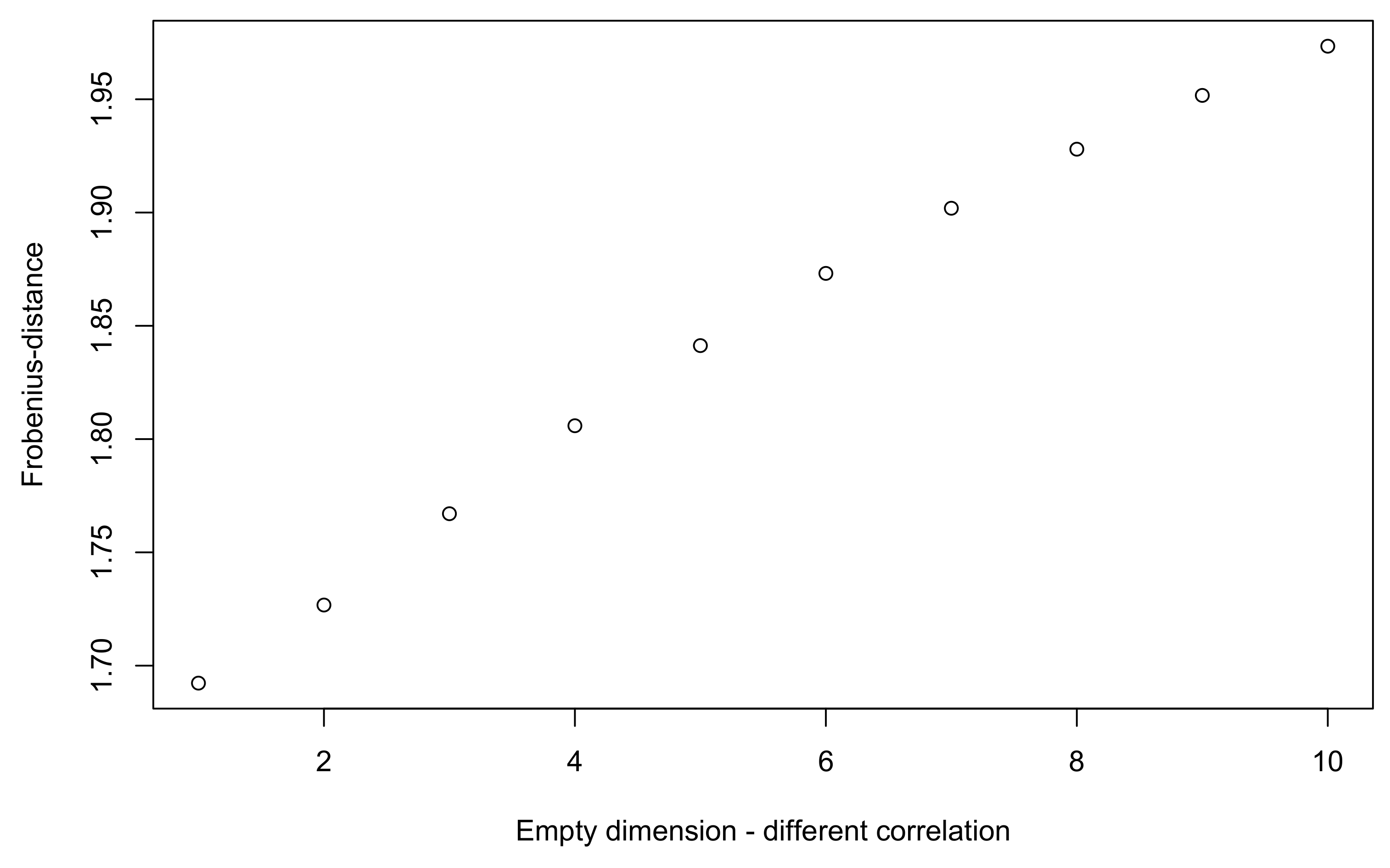
4.2. Adding a Risk: Increase the Matrix Dimension

Another arbitrary element chosen by the actuaries of the company is the number of risk factors to be aggregated. In some cases, it may be necessary to model many risk factors, according to the use of the internal model that is made by the business units (need to model many lines of business when modelling the reserving loss factor for instance). These choices have to be made for risk factors that are not material at Group level, even if they can be important for the concerned subsidiaries. Nevertheless, these choices will impact the final SCR through the modification brought to the overall correlation matrix during PSDization. Still based on the same example, let us consider the following case:

$$\left(\begin{array}{ccc}1& -0.9& -0.5\\ -0.9& 1& -0.5\\ -0.5& -0.5& 1\end{array}\right)\to \left(\begin{array}{cccc}1& -0.9& -0.5& 0.1\\ -0.9& 1& -0.5& 0.1\\ -0.5& -0.5& 1& 0.1\\ 0.1& 0.1& 0.1& 1\end{array}\right).$$

As can be noticed, the correlation is low between the added and the other risks.

Direct PSDization obviously gives the same results, whereas correlation coefficients are slightly modified after PSDization when introducing the new risk (see

Table 4. Modification of initial correlation coefficients due to the addition of a new risk.

Coef.	Before PSDization	Direct PSDization	PSDization with Higher Dimension
${\rho }_{12}$	$-0.9$	−0.585	−0.577
${\rho }_{13}$	−0.5	−0.473	−0.471
${\rho }_{23}$	−0.5	−0.437	−0.435

). Changes to these coefficients are difficult to anticipate, but it seems that the impact is lower in this case than with permutations. A natural question would be to understand whether the value of the correlation coefficient that was added is key to explaining the modifications obtained in the PSDized correlation matrix. Figure 2 shows this impact on the Frobenius norm, with a new risk with correlation coefficients that vary from 0.1 to 1. Results are intuitive: the higher the coefficients added, the wider the Frobenius norm. PSDization is indeed a whole process that takes into account every coefficient, including the one that was added.

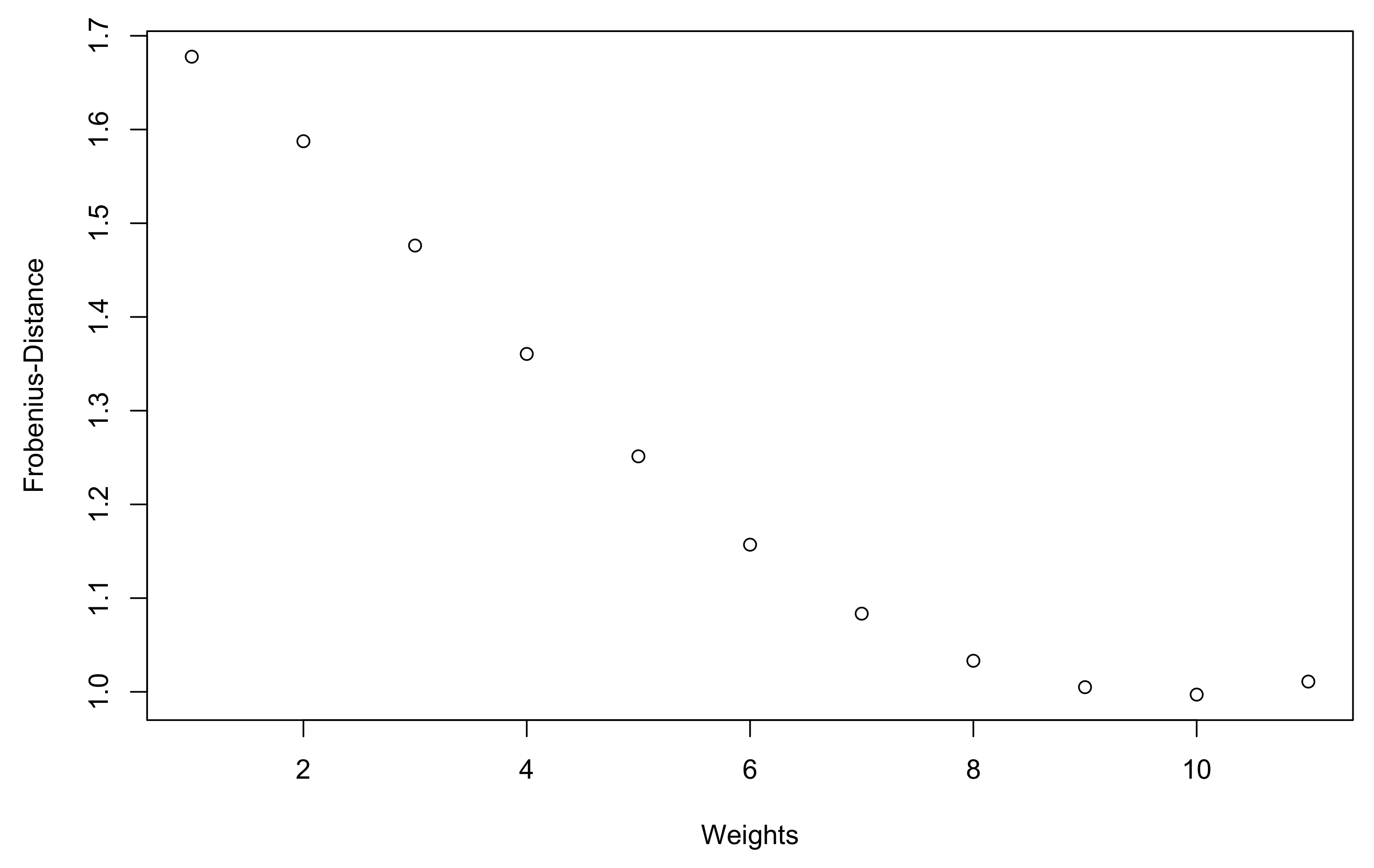
4.3. Impact of Confidence Weights

Finally, the choice of the weights associated to the terms of the correlation matrix, which somewhat represents the confidence level given by experts to the individual correlation coefficients, can also have a significant impact on the PSDized matrix. To illustrate this, still keeping in mind the example $G_{31}$ with the initial weights listed in $H^{init}$, we consider the new following weights:

$$\left(\begin{array}{ccc}{\omega }_{11}& {\omega }_{12}& {\omega }_{13}\\ {\omega }_{21}& {\omega }_{22}& {\omega }_{23}\\ {\omega }_{31}& {\omega }_{32}& {\omega }_{33}\end{array}\right)=\left(\begin{array}{ccc}1& 0.2& 0.8\\ 0.2& 1& 0.4\\ 0.8& 0.4& 1\end{array}\right).$$

The PSDized matrix is now given in

Table 5. Modification of initial correlation coefficients due to the introduction of weights.

Coef.	Before PSDization	PSDized (Initial Weights)	PSDization with New Weights
${\rho }_{12}$	$-0.9$	$-0.585$	$-0.642$
${\rho }_{13}$	−0.5	−0.473	−0.463
${\rho }_{23}$	−0.5	−0.437	−0.381

:

Clearly, correlation coefficients significantly vary. It illustrates that, as expected, the lower the weight, the further the modifications are from the initial coefficient. An increased weight on some correlation coefficients clearly leads to an increased importance in the PSDization process, and thus less modification for them (so as to minimize the Frobenius norm). To generalize and better understand to which extent the weights could impact the correlation coefficients after PSDization, Figure 3 shows the Frobenius norm between the solution $S_{51}^H$ and the initial matrix $G_{51}$, with weights varying from $H_{51}$ to a limit weighting matrix given by

$$H^{limit}=\left(\begin{array}{ccccc}1& 0.5& 0.5& 0.5& 0.5\\ 0.5& 1& 0.2& 0.5& 0.5\\ 0.5& 0.2& 1& 0.6& 0.6\\ 0.5& 0.5& 0.6& 1& 0.1\\ 0.5& 0.5& 0.6& 0.5& 1\end{array}\right).$$

This limit weighting matrix is used for illustration purposes only. It corresponds to increasing linearly by $+0.4$ the lowest weights of the matrix $H_{51}$, while decreasing the highest weights by the same factor. Figure 3 shows that the Frobenius norm decreases as the weighting matrix is distorted towards the limit $H^{limit}$, and a closer analysis reveals that this phenomenon is mainly due to the correlation coefficients ${\rho }_{24}$, ${\rho }_{25}$, ${\rho }_{34}$ and ${\rho }_{35}$ of $G_{51}$ (and their transposed coefficients), which exhibit lesser modifications than with the initial weighting matrix since their weights are significantly increased: from 0.1 to 0.5 and respectively from 0.2 to 0.6.

4.4. Summary and Comments on the Other Two Algorithms

To put it in a nutshell, Figure 4 shows the impact of permutations and weights (the two most prominent operations) on the Frobenius norm, in the conditions stated above. It shows that the impact on the norm is more important when weights vary than when the order of risk factors is changed.

In addition, it must be noted that low dimensions are used in this publication so as to keep computation time at an acceptable level, but when dimensions increase, the initial matrix can be farther from the PSD target. Indeed, Gerschgorin’s circle theorem states that $\forall G\in {\mathbb{C}}^{n\times n}$, $\forall \lambda \in$ Spec(G), $\exists i\in 〚1;n〛$ such as ${\displaystyle \lambda \in \{z\in \mathbb{C},|z-g_{ii}|\le \sum _{j\ne i}|g_{ij}|\}.}$ In particular, if G is a pseudo-correlation matrix of dimension $n\times n$, its eigenvalues $\lambda$ belong to the interval $[2-n;n]$. To illustrate this practically, a matrix $G_{100}$ of size $100\times 100$ was randomly generated (defined as the symmetric part of an initial matrix with 10,000 valuesbetween −1 and 1, and diagonal coefficients forced to 1). The matrix thus obtained has 43 negative eigenvalues, where the lowest one equals −6.74. In this case, $G_{100}$ must be significantly transformed to become PSD: for all three algorithms, the most modified coefficient changes from 0.96 to 0.10. Nevertheless, the AP and the Newton algorithms still give overall better results than the Rebonato–Jäckel algorithm:

$$\left|\right|S_{100}^{PA}-G_{100}{\left|\right|}_2=\left|\right|S_{100}^N-G_{100}{\left|\right|}_2=28.969\le \left|\right|S_{100}-G_{100}{\left|\right|}_2=29.015.$$

Furthermore, according to the authors’ observations, permutations do not affect the PSD solution when using the AP or the Newton algorithms, whatever the dimension of the correlation matrix. The previously observed sensitivity to permutations is due to the convergence of the Rebonato–Jäckel algorithm to a local minimum. Since a PSD matrix remains PSD after permutations, and since the norms studied do not change under permutation, the PSD solution should remain the same before and after permutation (provided that the algorithm used reaches the absolute minimum). It is therefore expected that the known extensions of the Newton algorithm to integrate weights would not generate a significant sensitivity to permutations.

Finally, let us mention that our conclusions about the addition of a new risk dimension apply to all algorithms. Adding a new dimension modifies the eigenvalues, and can thus require further transformations to become PSD. However, the ability to use weights can help reduce this impact. For example, when adding an empty dimension to $G_{51}$ with a 10% correlation between the initial and the added risk factors, the ability to set weights associated to this new dimension to 0 (instead of 1 for all other correlation coefficients) enables the Rebonato–Jäckel algorithm to reach the nearest solution:

$$\left|\right|S_{51ed}^H-G_{51ed}{\left|\right|}_H=0.991\le \left|\right|S_{51ed}^{PA}-G_{51ed}{\left|\right|}_H=\left|\right|S_{51ed}^N-G_{51ed}{\left|\right|}_H=0.996.$$

After these illustrations, we can now move on to the analysis of such transformations on the capital requirement.

5. Analysis of Solvency Capital Requirement Sensitivity

The importance of PSDization on the final correlation matrix (to be used to assess the insurer’s own funds requirement) has now been highlighted. The correlation coefficients chosen by the experts, or even those defined by statistical means can be significantly modified. The aim of this section is to provide some real-life sensitivities concerning the computation of the global SCR thanks to internal models. We would like to see SCR as a function of the main parameters in the actuary’s hand.

To carry this out, genetic algorithms are used to find a range $[min,max]$3 of values to which the SCR belongs; given a copula, realizations of risk factors, and proxy functions (more details later). The implemented algorithms are detailed in Appendix D.1 and Appendix D.2, respectively, for the case of permutations and weights. They correspond to an adaptation of the Rebonato-Jackël algorithm that incorporates these operations. At the end, the range is obtained for a given pseudo-correlation matrix G, a given weighting matrix H, and possibly a given permutation $\sigma$. Hence, we want to evaluate the function g such that $g:(G,H,\sigma )\to g(G,H,\sigma )=SCR\left(PS{D}_H(\sigma .G)\right)$, where $\sigma .G$ stands for the effect of $\sigma$ on the risk factors represented in G, and $PS{D}_H\left(G\right)$ represents the nearest (from G) PSD matrix obtained using the Rebonato-Jackël algorithm with weights H. The considered permutation $\sigma$ was presented at the beginning of Section 4.1.

5.1. Loss Factors or Risk Factors?

It must first be stated that estimating the loss generated by the occurrence of some given risk is a difficult task. It is easier to describe the behavior of risk factors through marginal distributions. For instance, if the interest rates rise, the potential loss for the insurer depends on impacts on both assets (e.g., value of obligations drops) and liabilities (contract credited rates may vary, which should modify expected lapse rates). To compute the loss associated to the variation of some risk factors, one thus needs a (very) complex transformation. In practice, to save computation time, simple functions (polynomial form) approximate these losses. However, the insurer can sometimes directly evaluate the loss related to one given loss factor: this is the case for example when considering the reserve risk, which can be modeled by classical statistical methods (bootstrap). The insurer’s total loss, P, thus reads

$$P=11_{\mathcal{R}\ne \varnothing }f\left({\left(X_i\right)}_{i\in \mathcal{R}}\right)+11_{\mathcal{P}\ne \varnothing }\sum _{i\in \mathcal{P}}{X}_j,$$

where f is a given (proxy) function, $X_i$ and $X_j$ are random variables, $\mathcal{P}$ is the set of loss factors and $\mathcal{R}$ is the set of risk factors.

For our next analysis,

Table 6. Polynomials used as proxy functions to obtain the overall insurer’s loss.

Dimension	Functional Form under Consideration
3	$P=f\left({\left(X_i\right)}_{i\in [1,3]}\right)=0.5X_1^2+2X_2^4+0.3X_3+10X_1{X}_2$
4	$P=f\left({\left(X_i\right)}_{i\in [1,4]}\right)=5X_1+0.02X_2^2+2000X_3+5X_4^{3/2}$
5	$P=f\left({\left(X_i\right)}_{i\in [1,5]}\right)=X_1+0.1X_2^2+50X_3+X_4^{1/2}-1.2X_5$
10	$P=f\left({\left(X_i\right)}_{i\in [1,10]}\right)=0.5X_1^3+0.4X_2^3+3X_3^2+2X_4^2+{\sum }_{i=5}^7{X}_i^2+0.5X_8^2+{\sum }_{i=9}^{10}{X}_i$

gives the different functional forms depending on the risk dimension and the risk factors $X_i$. For the sake of simplicity, one considers that all our marginals ($X_i$ and $X_j$) follow the same distribution but with different parameters. This common distribution is lognormal $\mathcal{LN}(\mu ,\lambda )$, since it is widely used in insurance for prudential reasons.

Table 7. Marginals for each risk factor and corresponding 99.5th percentile.

Name	Dim.	Parameters	${\mathit{X}}_1$	${\mathit{X}}_2$	${\mathit{X}}_3$	${\mathit{X}}_4$	${\mathit{X}}_5$	${\mathit{X}}_6$	${\mathit{X}}_7$	${\mathit{X}}_8$	${\mathit{X}}_9$	${\mathit{X}}_{10}$
$X_3^a$	3	($\mu ,\lambda$)	(6,0.5)	(5,0.5)	(4,0.1)
		$Q_{99.5}$	1463	538	71
$X_3^b$	3	($\mu ,\lambda$)	(6,0.8)	(3,0.1)	(12,2)
		$Q_{99.5}$	3167	26	28,110,637
$X_4^a$	4	($\mu ,\lambda$)	(6,0.5)	(5,0.5)	(4,0.1)	(3,0.9)
		$Q_{99.5}$	1463	538	71	204
$X_4^b$	4	($\mu ,\lambda$)	(1,5)	(2,4)	(3,3)	(1,4)
		$Q_{99.5}$	1,065,704	2,20,426	45,592	81,090
$X_5^a$	5	($\mu ,\lambda$)	(6,0.5)	(5,0.5)	(4,0.1)	(4,0.9)	(3,0.3)
		$Q_{99.5}$	1463	538	71	555	43
$X_5^b$	5	($\mu ,\lambda$)	(1,3)	(2,2)	(1,1)	(2,4)	(1,3)
		$Q_{99.5}$	6170	1276	36	220,426	6170
$X_{10}^a$	10	($\mu ,\lambda$)	(6,0.5)	(5,0.5)	(5,0.2)	(6,0.1)	(4,0.3)	(5,0.6)	(5,0.5)	(5,0.4)	(5,0.3)	(6,0.3)
		$Q_{99.5}$	1463	538	248	522	118	696	538	416	321	874
$X_{10}^b$	10	($\mu ,\lambda$)	(1.2,2)	(2,1.5)	(0.3,2.5)	(2,2)	(1.5,2)	(3.5,1)	(1.5,2)	(2.5,2)	(5,2)	(6,2)
		$Q_{99.5}$	573	352	845	1276	774	435	774	2104	25,633	69,679

sums up the parameters involved in the eight different cases under study: vectors $X_k^a$ (where k refers to the dimension of the vector) will be used to compute the global loss in the case of loss factors aggregation (meaning that $\mathcal{R}=\varnothing$), whereas vectors $X_k^b$ will be the input of proxy functions defined in Table 6 for risk factors aggregation ($\mathcal{P}=\varnothing$). We distinguish these two configurations to see whether taking into account proxy functions gives very different SCR sensibilities as compared to only aggregate risk factors.

5.2. Variance–Covariance or Copula Approach, Pros and Cons

Except for the PSDization step itself; which generates different results, another important choice lies in the aggregation approach. Here, one would like to detail the reasons for choosing one of them (i.e., copula or variance–covariance). Let us consider the simplest framework: the loss P only depends on loss factors (no need to apply proxy functions that link risk factors to loss factors). It is then possible to model this loss as follows: $P={\sum }_{i\in \mathcal{P}}{X}_i$.

Individual loss factors have to be modeled and estimated by the actuaries for internal models, or come from standardized shocks if using the Standard Formula. Fortunately, it is likely that extreme events corresponding to the 99.5th percentile of every loss factors do not occur at the same time: there is thus a mitigation effect, which generally implies

$$q_{99.5\%}\left(P\right)\le \sum _{i\in \mathcal{P}}{q}_{99.5\%}\left(X_i\right).$$

As already mentioned in Section 1, the regulation states that the variance–covariance approach can be used to aggregate risks, with the given correlation matrices. This method has some advantages, but also some drawbacks (Embrechts et al. 2013). Of course, it is the easiest way to aggregate risks: the formula is quickly implemented (which allows for computing sensitivities without too much effort), and easy to understand. However, it does not provide the entire distribution of the aggregated loss, knowing that the insurer is sometimes interested in other risk measures than the unique 99.5th percentile. Moreover, this approach is not adequate for modelling nonlinear correlations, which are common when considering the tails of loss distributions. It means that it is very tricky to calibrate the correlation matrix so as to ensure that we can effectively estimate the 99.5th percentile of the aggregated loss. In their paper, Clemente and Savelli (2011) and Sandström (2007) discussed this and proposed a way to modify the Solvency II aggregation formula in order to consider skewed marginal distribution. Finally, the variance–covariance approach is too restrictive since it does not allow the correlation of risk factors, but only the correlation of losses. This makes the interpretation of scenarios generating a huge aggregated loss very difficult.

For all these reasons, internal models are generally developed using copulas: they enable the simulation of a large number of joint replications of risk factors, before applying proxy functions (most of the time). With this technique, insurers obtain the full distribution of P, and thus richer information among which is the quantile of interest (Embrechts and Puccetti (2010), Lescourret and Robert (2006)). Common copulas in the insurance industry (Gaussian and Student copulas) are based on the linear correlation matrix, the marginals being the risk and loss factors. This is linked to the main property of copulas: they allow the definition of the correlation structure and the marginals separately. For example, aggregation with the Gaussian copula can be simulated with the following steps:

• simulation of the marginals stand-alone (stored in the vector $X\in {\mathbb{R}}^{n\times B}$, where n stands for the number of risk factors and B the number of random samples);
• simulation of a Gaussian vector Y through the expression $Y=TZ$, where T represents the Choleski decomposition of the correlation matrix $\rho ={\left({\rho }_{ij}\right)}_{(i,j)\in 〚1,n〛}$ and Z is an independent Gaussian vector of size n;
• ordering X in the same order as Y to ensure that $\forall j\in \{1,\dots ,B\},\forall i\in \{1,\dots ,n\},q\left(X_{ij}\right)=q\left(Y_{ij}\right)$ ($q\left(x\right)$ stands for the quantile corresponding to x).

5.3. Results Using a Simplified Internal Model

Applications presented hereafter were designed to consider a wide range of operational situations in which the insurer aims to estimate its global SCR.

For a given PSD correlation matrix $S_{xy}^H$, and given values for the vector of risk factors (simulated with lognormal distributions), one performs Q = 131,072 = $2^{17}$ simulations for the aggregation of risk factors (dependence structure). As a matter of fact, there are two sources of uncertainty explaining the variation of SCR values ($SCR={\left(SC{R}_q\right)}_{q=1,\dots ,Q}$). First, the genetic algorithm itself is likely to have reached different local solutions depending on the simulation. Second, the simulation of the Gaussian or Student vectors to model the correlation through copulas may change. In order to focus the study on correlation, it must be noted that marginals were simulated initially and then kept fixed. Roughly, it can be assumed that the confidence interval of the global SCR is similar to that of a Gaussian distribution ($SC{R}_q\sim SCR\sim \mathcal{N}(m,\sigma )$) because of the Central Limit Theorem and of the independence of the simulations of each SCR, i.e.,

$$\mathbb{P}\left(\right|SCR-m|<1.65\sigma )=90\%,$$

where $\sigma$ stands for the standard deviation of SCR, and m its mean. Of course, the estimation of these parameters is made simple using their empirical counterparts, denoted by $\widehat{m}=(1/Q){\sum }_{q}SC{R}_q$ and ${\widehat{\sigma }}^2=(1/(Q-1)){\sum }_q{(SC{R}_q-\widehat{m})}^2$.

Table 8. Mean and standard deviation of the global Solvency Capital Requirement (SCR) ($Q=2^{17}$ simulations).

		Gaussian Copula				Student Copula
						(3 degrees of freedom)
		Loss factors ${\mathit{X}}_{\mathit{k}}^{\mathit{a}}$		Risk Factors ${\mathit{X}}_{\mathit{k}}^{\mathit{b}}$		Loss Factors ${\mathit{X}}_{\mathit{k}}^{\mathit{a}}$		Risk Factors ${\mathit{X}}_{\mathit{k}}^{\mathit{b}}$
Example	Dim. $\mathit{k}$	$\widehat{\mathit{m}}$	$\widehat{\mathit{\sigma }}$	$\widehat{\mathit{m}}$	$\widehat{\mathit{\sigma }}$	$\widehat{\mathit{m}}$	$\widehat{\mathit{\sigma }}$	$\widehat{\mathit{m}}$	$\widehat{\mathit{\sigma }}$
$S_{31}^H$	3	2566	0.06%	12,119,354	0.16%	2576	0.11%	12,473,296	0.32%
$S_{32}^H$	3	2694	0.08%	13,808,174	0.19%	2813	0.20%	14,641,263	0.86%
$S_{41}^H$	4	3319	0.10%	3,532,563	0.10%	3379	0.16%	3,555,426	0.33%
$S_{42}^H$	4	2809	0.14%	3,563,414	0.31%	2997	0.29%	3,578,124	0.35%
$S_{51}^H$	5	2605	0.09%	9359	0.68%	2677	0.18%	9411	0.59%
$S_{52}^H$	5	3139	0.13%	8303	0.28%	3260	0.32%	8531	0.99%
$S_{101}^H$	10	5825	0.26%	4,174,500	0.73%	6717	0.31%	4,234,635	1.14%

summarizes the estimated quantities for each case in our framework.

Then, we study the impact of our transformations (permutation, weights varying, and higher dimension) as compared to this standard deviation $\widehat{\sigma }$. More precisely, we consider one operation, perform the same number of simulations, and store the minimum and maximum values of the vector ${\left(SC{R}_q\right)}_{q=1,\dots ,Q}$. This way, it is possible to define a normalized range (NR) for these values, as expressed below:

$$NR=\frac{max\left(SCR\right)-min\left(SCR\right)}{\widehat{m}}.$$

(2)

If NR is lower than ($2\times 1.65\times \widehat{\sigma }$), the transformation is said to have a limited impact on the SCR. Otherwise, it is considered as a significant impact. The worst cases correspond to situations where NR is greater than ($2\times 2.89\times \widehat{\sigma }$). The multiplier 2 enables us to take into account the fact that there are two sources of uncertainty (genetic algorithm and simulated dependence structure). All the results are stored in

Table 9. Sensitivities of the global SCR to transformations on the correlation matrix (permutation, two different cases for weighting the correlation coefficients, and addition of a new risk), depending on copula, and type of aggregation (risk factors/loss factors). Column ‘Imp.’ describes the strength of the impact of the transformation under study: ‘0’ refers to a limited impact ($NR<2\times 1.65\widehat{\sigma }$, see (2)), ‘+’ means a significant impact ($NR\in [2\times 1.65\widehat{\sigma },2\times 2.89\widehat{\sigma }]$), and ‘++’ a very strong impact ($NR>2\times 2.89\widehat{\sigma }$).

			Gaussian Copula								Student Copula
			Loss Factors ${\mathit{X}}_{\mathit{k}}^{\mathit{a}}$				Risk Factors ${\mathit{X}}_{\mathit{k}}^{\mathit{b}}$				Loss Factors ${\mathit{X}}_{\mathit{k}}^{\mathit{a}}$				Risk Factors ${\mathit{X}}_{\mathit{k}}^{\mathit{b}}$
	$\mathit{k}$	Operation	$\mathit{SCR}$min	$\mathit{SCR}$max	NR	Imp.	$\mathit{SCR}$min	$\mathit{SCR}$max	NR	Imp.	$\mathit{SCR}$min	$\mathit{SCR}$max	NR	Imp.	$\mathit{SCR}$min	$\mathit{SCR}$max	NR	Imp.
$G_{31}$	3	Permut.	2562.64	2572.78	0.4%	++					2565.31	2589.81	0.95%	++
		W Sensi1	2564.11	2577.68	0.53%	++	12,081,399	12,120,187	0.32%	0	2575.71	2608.43	1.27%	++	12,326,216	12,469,140	1.16%	+
		W Sensi2	2560.19	2565.96	0.23%	+	12,072,651	12,135,251	0.52%	0	2565.05	2575.55	0.41%	+	12,382,841	12,486,700	0.84%	0
			initial:	final:			initial:	final:			initial:	final:			initial:	final:
		dim+1	2593.96	2568.93	0.99%	++	12,132,660	12,249,386	0.96%	++	2576.77	2578.86	0.08%	0	12,435,526	12,568,778	1.07%	+
$G_{32}$	3	Permut.	2635.26	2758.19	4.66%	++					2726.01	2891.99	6.09%	++
		W Sensi1	2627.97	2665.76	1.44%	++	12,447,404	12,829,070	3.07%	++	2705.99	2749.83	1.62%	++	13,758,628	14,050,626	2.12%	0
		W Sensi2	2675.38	2693.56	0.68%	++	12,765,514	12,971,883	1.62%	++	2784.25	2803.88	0.70%	+	14,133,464	14,656,943	3.70%	+
		dim+1	2709.62	2694.79	0.55%	++	13,127,451	13,249,432	0.93%	+	2802.37	2805.6	0.12%	0	14,704,558	14,623,516	0.55%	0
$G_{41}$	4	Permut.	3293.26	3356.76	1.93%	++					3354.11	3429.74	2.25%	++
		W Sensi1	3121.05	3232.06	3.56%	++	3,516,332	3,532,352	0.46%	+	3288.28	3325.72	1.14%	++	3,515,774	3,541,524	0.73%	0
		W Sensi2	3297.22	3320.04	0.69%	++	3,520,161	3,532,792	0.36%	+	3360.15	3378.96	0.56%	+	3,517,889	3,541,680	0.68%	0
		dim+1	3228.74	3323.74	0.17%	0	3,529,310	3,534,685	0.15%	0	3364.13	3572.28	6.19%	++	3,533,674	3,541,166	0.21%	0
$G_{42}$	4	Permut.	2759.38	2824.89	2.37%	++					2909.99	3011.72	3.50%	++
		W Sensi1	2814.42	2905.75	3.25%	++	3,519,944	3,551,629	0.90%	0	2995.14	3060.68	2.19%	++	3,509,471	3,555,086	1.30%	+
		W Sensi2	2803.70	2828.836	0.90%	++	3,540,453	3,565,096	0.70%	0	2933.73	2996.47	2.14%	++	3,521,590	3,555,627	0.97%	0
		dim+1	2814.497	2801.376	0.47%	+	3,564,593	3,561,905	0.08%	0	2996.24	2999.27	0.10%	0	3,549,029	3,529,009	0.56%	0
$G_{51}$	5	Permut.	2607.65	2627.15	0.75%	++					2658.80	2700.28	1.56%	++
		W Sensi1	2637.39	2662.24	0.94%	++	8541.412	8931.55	4.57%	++	2697.89	2745.08	1.75%	++	8768.985	9148.675	4.33%	++
		W Sensi2	2607.38	2616.21	0.34%	+	9201.858	9328.433	1.38%	0	2660.28	2674.21	0.52%	0	9136.763	9394.289	2.82%	+
		dim+1	2615.5	2626.37	0.42%	+	9333.50	9336.61	0.03%	0	2670.86	2665.32	0.21%	0	9457.66	9409.49	0.51%	0
$G_{52}$	5	Permut.	2952.79	3152.47	6.76%	++					3113.23	3300.16	6.00%	++
		W Sensi1	2929.41	3088.92	5.45%	++	8230.70	8649.88	5.09%	++	3148.10	3241.26	2.96%	++	8444.65	8834.73	4.62%	+
		W Sensi2	3120.47	3141.46	0.67%	+	8180.51	8323.61	1.75%	++	3100.95	3248.25	4.75%	++	8339.17	8579.71	2.88%	0
		dim+1	3139.02	3145.94	0.22%	0	8291.98	8337.67	0.55%	0	3264.48	3228.87	1.09%	+	8473.53	8680.028	2.44%	0
$G_{101}$	10	Permut.	5767.08	5887.43	2.09%	++					6657.96	6837.03	2.69%	++
		W Sensi1	5716.66	5864.03	2.58%	++	4,096,899	4,166,343	1.69%	0	6631.49	6737.25	1.60%	+	4,077,298	4,225,148	3.62%	+
		W Sensi2	5765.11	5816.17	0.89%	+	4,086,983	4,181,583	2.31%	0	6633.39	6728.64	1.44%	+	4,104,747	4,240,035	3.29%	+
		dim+1	5800.75	5811.27	0.18%	0	4,226,948	4,192,248	0.82%	0	6701.83	6753.39	0.76%	0	4,224,386	4,362,900	3.27%	0

.

5.3.1. Impact of Permutations on the Global Solvency Capital Requirement

Of the 14 examples under study (seven pseudo-correlation matrices $G_{xy}$ times Gaussian or Student copula, see Table 9), the permutation systematically has a very strong impact on the global SCR. This change can represent up to 6.7% in practice, although it should have no theoretical impact. This is mainly due to the PSDization process, which leads to the selection of different local minima after a permutation is made. This highlights two phenomenona: the need to control the bias induced by the initial choice of the insurer concerning the order of risk factors, and the need to initially define PSD correlation matrices (revisiting experts’ opinions, and identifying incoherent correlation submatrices).

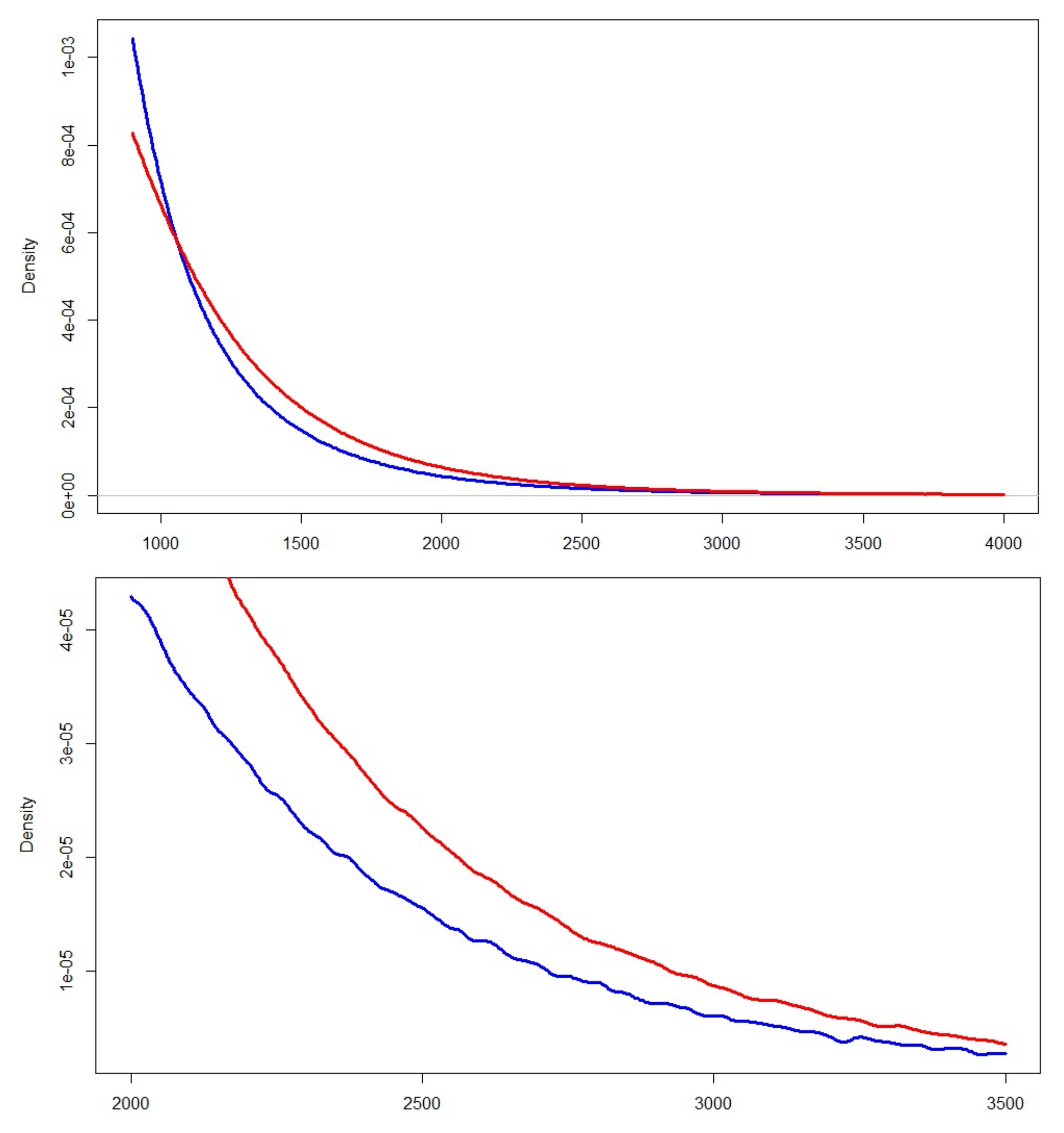
To have a more comprehensive view of this impact, Figure 5 illustrates it on the total loss distribution (rather than the sole 99.5th percentile), with $G_{52}$, $H_{52}$ and considering the aggregation of loss factors. The red curve corresponds to the loss distribution after applying the permutation $(1\mapsto 5;4\mapsto 1;5\mapsto 4)$ to $G_{52}$ in the case of a Gaussian copula, whereas the blue one corresponds to the permutation $(2\mapsto 3;3\mapsto 4;4\mapsto 5;5\mapsto 2)$.

5.3.2. Impact of the Modification of Weights on Solvency Capital Requirement

Our sensitivities relate to weighting coefficients varying in a given range. This range is defined by weights between $H^{min}={\left[0\right]}_{(i,j)\in 〚1,n{〛}^2}$ and $H^{max}={\left[1\right]}_{(i,j)\in 〚1,n{〛}^2}$. This sensitivity is denoted by ‘W Sensi1’ in Table 9. Of the 28 examples analyzed here, (seven pseudo-correlation matrices $G_{xy}$, times (Gaussian or Student copula), times (risk or loss factors)), 17 cases have a very strong impact on the SCR. The range $[SC{R}^{min};SC{R}^{max}]$ can represent more than 5.4% of the SCR, which is really huge in practice.

The same analysis with stronger constraints (weights belonging to an interval of width 0.2 around the initial weights, i.e., $H^{min}=H-{\left[0.1\right]}_{(i,j)\in 〚1,n{〛}^2}$ and $H^{max}=H+{\left[0.1\right]}_{(i,j)\in 〚1,n{〛}^2}$, see ‘W Sensi2’ in Table 9) shows that of 28 examples, seven cases have a very significant impact on the final SCR, with a range likely to represent more than 4.7% of the SCR. Furthermore, this shows the necessity to properly define correlation coefficients at the very beginning.

5.3.3. Impact of Adding a Dimension to the Correlation Matrix

In practice, the insurer’s global loss often incorporates some negligible loss factor. In the simple case where there are only loss factors affecting the global loss, it means that

$$P=\sum _{j\in \mathcal{P},j\ne n+1}{X}_j+ϵX_{n+1},$$

where $ϵ$ thus tends to 0. The limit case would be $ϵ=0$, which means that the (n+1)th risk factor would have no impact on the insurer’s loss, but still plays a role through its presence in the correlation matrix and its impact in the PSDization process. The correlation between this risk factor and others is set to 0.1 (as in Section 4.2). We measure the SCR value before and after adding this dimension.

Of the 28 examples analyzed (see ‘dim+1’ in Table 9), almost one third (nine cases exactly) lead to a statistically significant impact on the final SCR (strong or very strong impact on SCR). However, except in one specific case involving an impact value around 6%, most of the impacts seem to be lower than with other operations. Once again, it is important to realize that this transformation should have no theoretical impact. Of course, it suggests that it would be worth conducting deeper analysis on this aspect, especially on the addition of more than one dimension and on the modification of the correlation coefficients of the added risk factor.

6. Conclusions

Insurers using internal models, as well as supervisors, wonder quite rightly about the robustness of their PSDization algorithm. Our study shows and highlights the importance of PSDization through quantified answers to very practical questions on a series of real-life examples. Of the 98 (3 × 28 + 14) examples based on various configurations (different copulas and ways to consider risks, see Table 9), approximately one half (exactly 47) have significant impacts on the global SCR (up to 6%) when studying sensitivities to our three tuning parameters (weights given to individual correlation coefficients, permutations, and addition of a fictive business line). It can be noted that permutations always lead to a significant variation of the overall SCR, with a normalized range (see Equation (2)) often greater than in other cases. Adequate sensitivities should therefore be performed when using the Rebonato–Jäckel algorithm since there is to the authors’ knowledge no way to know a priori which would be the most adapted choice of risk order for a given company. Knowing that these transformations are either theoretically neutral, or should have a limited impact on the global capital requirement, this underlines that practitioners’ choices are fundamental when performing risk aggregation in internal models. Moreover, the use of proxy functions do not seem to change conclusions: SCR sensitivity is similar when considering only loss factors. A strong control of PSDization by supervisors thus makes sense, and a good understanding of the behaviour of the PSDization algorithm is required.

The following best practices were identified: (i) develop a sound internal control framework on both the triggers generating negative eigenvalues (e.g., expert judgments) and the PSDization step itself, and (ii) assess the need for adding a new risk (e.g., new business line) in terms of its impact on the correlation matrix and thus on the global SCR. Regarding the former point, independent validations and systematic reviews of the modifications brought to the correlation matrix by the algorithm should be analyzed, and a wide number of sensitivities has to be implemented to challenge the results. Concerning the dimension of the risk matrix, there seems to be a compromise to find: adding business lines allows for increasing granularity when describing the correlation between risks, but tends to cause more disturbance on the individual correlation coefficients during PSDization. As usual, the best choice lies in an intermediate dimension.

Finally, this work could be extended in several ways, among which the definition of algebraic tests to anticipate inconsistencies in the experts’ choices; and a deeper understanding of the permutations leading to the minimum or maximum values of the SCR. In particular, if these permutations show some similar features, it would be possible to define best practices when ordering risk factors.