1. Introduction
In several jurisdictions, anyone who owns a motor vehicle must have auto insurance coverage at all times. At a minimum, the insurance must provide some level of liability protection, although many motor vehicle owners opt for a more comprehensive coverage that additionally provides for insurance protection against collision and vehicle damage. The automobile insurance market is very competitive where motor vehicle owners can shop freely for insurance coverage that are generally homogeneous but prices are extremely competitive. For insurance companies then, customer loyalty and policy retention become an important strategic management because it is generally more cost efficient to retain existing policies than to acquire new ones (see
McClenahan (2001)).
It has long been held that when the policyholder made a claim in the prior year, the subsequent premium is likely to increase. The level of premium depends on many factors such as the frequency and severity of the claims made. In some jurisdictions, the practice of implementing a bonus-malus system allows for a well-defined mechanism of premium determination triggered by claims. In a bonus-malus system, premiums increase the following policy year whenever claims are made this policy year. On the other hand, discounted premiums are provided if there is no claim (see
Lemaire (1985)). In Singapore, their bonus-malus system is more formally referred to as a No-Claims Discount (NCD) system. It has a baseline premium with a 0% discount and discounts are provided in increments of 10% per year for up to 50%.
When claims trigger premium increase, it becomes more attractive for the policyholder to seek for another insurance company that may offer a more competitive premium thereby possibly avoiding bearing a higher premium. In such situations, insurers are faced with the challenges of policyholder retention by keeping premiums and possibly expenses low in the face of competition. For every line of insurance, understanding policyholder behavior is an important aspect in the overall operations of an insurance company (see
Campbell et al. (2014)). However, the effect of claims on policyholder behavior is quite unique to property and casualty insurance, especially for automobile insurance. The short term nature of the insurance coverage allows policyholders to easily decide whether to switch to another company.
Some work has been done to address the relationship between price and lapse. For example,
Dutang (2012) studied the effect of price changes on the renewal of non-life insurance contracts and pointed out that market proxies are important for lapse rate predictions.
Guelman and Guillén (2014) proposed a causal inference framework to measure price elasticity in the context of auto insurance and found that higher premiums lead to higher lapse rates.
Guelman et al. (2014) pointed out that many insurers would reduce their profits a little in order to increase their renewal rates.
Bolancé et al. (2018) investigated optimal prices for customers by assuming that prices have an impact on the probability of renewal.
The main focus of the aforementioned work is on profit maximization. The pre-existing notion of the relationship between policyholder claims and lapse has never been empirically investigated in the actuarial or insurance literature. There is a clear apparent reason for this. It is relatively challenging for insurance companies and researchers to explore this notion because such an analysis requires a follow-up of policyholders switching between companies and capturing the implications of this for analyzing behavioral pattern. Our Singapore dataset is unique and quite suitable for this type of analysis because the dataset contains detailed, micro-level automobile insurance records of all insurance companies in Singapore. It consists of records in three separate files over a nine-year period, covering years 1993–2001, of 45 insurance companies that sell automobile insurance coverage in the country. The policy file has over five million records of policy information, such as type of coverage, vehicle type, driver’s age and gender, for each registered car insured in each calendar year. The claims file has under a million records of claims that include dates and amounts of claims filed. The payment file has over four million records of dates, amounts and other useful information about payments made for claims that were filed and recorded in the claims file. Extracts of claims experience of different companies from this same dataset have been used for empirical investigation in
Frees and Valdez (2008) and
Frees et al. (2009).
In making this dataset useful for our purposes, we have extracted all the claims information, together with policyholder and vehicle characteristics, so that we are able to track the policy switch between calendar years. As part of the preparation of this dataset, the switch has been determined according to the identification of the vehicle information since contract identification cannot be unique among the insurance companies. Based on the dataset used in this paper, we have a total of 893,009 observations of which 324,182 have an indicated policy switch. A policy switch is a binary variable derived from the dataset that indicates an evidence that a policyholder has just changed to a different insurance company. We have removed the observations that did not provide us accurate evidence of switch. For example, there were vehicles for which we may have lost trace possibly because these were sold so that someone else became a new owner of the vehicle with a new vehicle identification.
Now for uncovering interesting relationships between insurance claims and policy switch, we employ a data mining methodology called
association rule learning. This technique has its origins in the retail industry where a huge amount of data on customer purchases were analyzed to understand consumer buying behavior (see
Agrawal et al. (1993)). This data analysis can come in the form of an association rule about relationships of the items purchased. To illustrate, the rule
may be drawn from the dataset to suggest that there is a strong likelihood of purchasing tomatoes when ground beef and bun are purchased together. Such mining of information can provide valuable insights to businesses for further promotions and sales, for improving customer relations, and for better management of its product inventories.
Despite its conceptual simplicity, association rule learning has potential applications for a more effective data-driven decision making in a wide variety of disciplines including medical diagnosis, credit card fraud detection and health informatics (see
Rajak and Gupta (2008) and
Altaf et al. (2017)). Using association analysis, a physician may find association of symptoms for more accurate diagnosis of illness for better patient care. On a similar note,
Kost et al. (2012) used this method to derive associations among diseases so that they can compare co-occurrences of diseases at the different levels. Using the data from the 2009 Vernon Uniform Hospital Discharge Data Set with the ICD-9-CM codes to classify diagnoses, the authors were able to identify associations overlapping and new associations among diseases.
In
Wong et al. (2005), association rule learning was used and applied in order to achieve optimal direct marketing. It is very important to choose appropriate customers for sending marketing mails because sending mail requires costs. In their paper, they used modified association rule learning and achieved 3.3 times of the profit per mail relative to that of naive method.
It is possible to find an application of association rule learning in actuarial science as well.
Lau and Tripathi (2011) used the technique to derive associations between the characteristics of workers and claim types in worker’s compensation insurance. They conducted association rule learning on the historical claim data of a waste management company and they find some significant rules, such as
and
. By having an understanding of the pattern of the event leading to injuries, the company and the insurers may help determine changes in safety processes in order to prevent future injuries and thereby provide economic incentives.
Association rule learning originated from the work of
Agrawal et al. (1993). It is the objective of this technique to mine a big dataset and to draw a connection of the values of the variables in the dataset. Such connection is expressed as an implication of the form
where the left-hand side (lhs) A is called the antecedent while right-hand side (rhs) B is called the consequent. The antecedent is a statement of a premise that the condition stated as a consequent is true. The degree of seriousness of this implication can be measured in several ways as discussed in the body of this paper. The purpose of this is straightforward: to mine our Singapore market insurance data to provide us empirical evidence of the relationships among insurance claims, the premium immediately following a claim, and lapse behavior. Ignoring the policyholder and vehicle characteristics, we controlled for in our analysis, our results provided strong evidence of relationships and we were able to deduce association rules in the form:
We will briefly mention that other more traditional approaches of supervised learning would have made it difficult, if not impossible, to draw such evidence. In traditional approaches of supervised learning (e.g., linear models, generalized linear models), we already have some ideas about the relationships among the variables so that we can come up with some models. In contrast to these traditional approaches of supervised learning, association rule learning is more suitably used as an exploratory tool as we have done so in this paper. In association rule learning, we aim to find some relationships among the variables so that we can use them to build predictive models in the next step. As a result, we caution the reader and user of our results that association rules are difficult to use as predictive models.
For the rest of this paper, it has been organized as follows.
Section 2 provides an overview about association rule learning. We also define the measures commonly used in association rules.
Section 3 provides discussion and summarization of the dataset used in our empirical investigation.
Section 4 details the results of our analysis. We conclude in
Section 5.
2. Concepts of Association Rule Learning
Consider a set
of
m items where
, and denote the dataset
D to be the set of all
N transactions represented as
. The items are sometimes called attributes that are often binary variables but could also be categorical variables. None of the items can be continuous and the practice is to convert continuous into categorical variables for meaningful applications of association rule learning. The transaction
in the dataset, for
, is a subset of items from the dataset. An itemset
X is a collection of zero or more items and we can call the null (or empty) set to be the itemset with zero items. If the itemset
X is a subset of transaction
, then we say that the transaction contains the itemset
X (see
Bramer (2016) and
Weiss et al. (2010)).
Given association rule learning has its origin in marketing, the dataset is usually a market basket data with items referring to goods or products purchased. See, for example, the work of
Agrawal et al. (1993). For our purposes of illustration, consider the simplified course enrollment data example tabulated in
Table 1.
Each of the eight students in this dataset can enroll in any of the five subjects: Calculus, Physics, Statistics, Latin, and History. The subjects are the items in our dataset, each of which is a binary attribute that indicate enrollment in the subject. A value of 1 indicates enrollment in the corresponding course whereas 0 means no enrollment. The listing of courses for each student are the transactions in our dataset; we therefore have a total of eight transactions with each corresponding to a student. For example, Student ID 3 has the transaction while Student ID 6 has the transaction . The itemset is a subset of transactions , , and .
Such a course enrollment dataset can provide meaningful information to a university to understand its enrollment pattern in order to meet enrollment needs. Planning for enrollment needs is critical to a university to optimally allocate scarce resources. One of the decision making process for this purpose is to derive meaningful association rules among the different courses. An association rule is indeed expressed as an implication of the form for disjoint itemsets X and Y, that is, . If all m possible items are binary attributes, there would be a total number of possible association rules. In our enrollment dataset with five courses (or attributes), this leads us to a total of 80 possible association rules. Evaluating the interestingness and strength of each possible association rule can clearly be costly and this cost increases exponentially with the number of attributes present.
Association rule learning is a data mining method for finding meaningful relations among incidence of events with information extracted from these incidences. For our course enrollment dataset, association rules can help the university draw conclusions from queries that are for example:
Search for association rules with “Statistics” as the antecedent. Such rules can help the university assess the impact of deciding to discontinue offering this course.
Search for association rules with “Physics” as the consequent. Such rules can help the university plan for courses that will lead to an increased enrollment for this course.
Search for association rules with “Statistics” as the antecedent and “Physics” as the consequent. Such rules can help the university plan for subjects in addition to “Statistics” that will help further boost enrollment for “Physics”.
Search for the most attractive, or best, association rules with “Physics” as the consequent. Best can be measured according to the interestingness or strength of such rules.
2.1. Common Measures Used
There are important measures used in association rule learning to assist the decision maker in drawing the strength and interestingness of an association rule.
To begin, we introduce the concept of a
which measures the frequency of an itemset. The support of an itemset
X is defined as the proportion of observations which contains
X in the whole dataset. Mathematically, we write
where
refers to the number of elements in the set. Using our sample dataset, the support of the itemset
is
. Support can be an important measure because infrequent itemsets, those with low support, may be immediately discarded or eliminated in mining for association rules. Those itemsets with large support are more highly desirable.
Confidence is a measure that is based on the notion of a support. For a given rule, say
, we define confidence as:
For a given rule , this reliability measure gives us the proportion of the observations in our dataset with all items from X that have also all items from Y. The larger this proportion is, the more confident we are for the itemset Y to be present in our observations that contain itemset X. In our sample dataset, for the rule we have a confidence of . In words, among those students who enroll in both Physics and Statistics, 75% of the time they will also enroll in Latin.
There are two additional measures of interestingness of association rules that we would like to use in this paper. We define the metric
of a rule as follows:
It is computed as the ratio of the confidence to the support of the consequent in the rule, but it can also be expressed as the ratio of the support of to the product of the support of X and the support of Y. This latter expression provides us an interesting interpretation of the lift: if the events associated with the itemsets X and Y are independent, then there is no possible association rule that can be drawn. In effect, the lift is a measure of the degree to which there is presence of dependence.
A lift of 1 indicates there is independence. A lift > 1 indicates a strong presence of dependence in which case, the association rule is much more potentially useful. In our sample dataset, for the rule , we have a lift of . In this case, an association rule can be meaningfully drawn from with X as the antecedent and Y as the consequent.
Finally, the
of a given rule is defined as
Conviction is a metric that is used to measure the strength of the association between X and Y than just completely random. The numerator is the frequency of the occurrence of X in the absence of Y in the case of independence. The denominator is the total frequency of X in the absence of Y. Using our sample enrollment dataset, for the rule , we have a conviction of .
By re-writing the conviction formula as
we can show the relationships among conviction, confidence, and the lift as follows:
Especially for interpretation purposes, it may be imperative to express these metrics in probabilistic terms. By defining
and
to be the respective events of having itemsets
X and
Y, we have a summary of the equivalence
Table 2.
The association rule metrics are estimates of the corresponding probabilities in this table. For example, the support of X is an estimate of the probability that an observation in the dataset (or transaction) contains the itemset X. In addition, the confidence is an estimate of the probability that an observation contains the itemset Y, given it contains X.
2.2. The Algorithm
Association rule data mining techniques involve the process of searching for frequent itemsets in the dataset that satisfy a support threshold and then extracting rules from these frequent itemsets. It can be rephrased as a technique involving two tasks:
Find all the itemsets X which satisfies , where is a minimum level of required support as determined according to the purpose of analysis.
Utilizing these frequent itemsets, find all the association rules which satisfies , where is a minimum level of required confidence.
For details, see
Agrawal et al. (1993). Note that although the common practice is to specify a minimum threshold for confidence, because of the relationship among confidence, lift, and conviction, as shown in the previous subsection, this is equivalent to specifying thresholds of these other measures.
Accomplishing the tasks involved in association rule learning can be rather straightforward by searching our dataset for all itemsets and all possible association rules that meet these thresholds. Even with the aid of fast computing, this brute-force approach of searching all possibilities can lead to infinitely many rules that can be difficult to extract and to draw meaningful deductions. One of the earliest and simplest association rule algorithm, the approach can provide assistance in this regard with an algorithm that reduces the candidate itemsets for consideration of association rules. This reduction procedure, known as support-pruning, is accomplished by iteratively eliminating itemsets that do not satisfy the pre-specified threshold. For an itemset that is considered frequent, then all of its subsets must also be infrequent. The elimination process, according to this principle, is therefore exercised by removing infrequent itemsets when the converse of this principle is applied.
To demonstrate the effectiveness of this pruning process, consider a dataset with a list of say 10 items. The initial phase of the process is to consider all 1-itemsets, remove the infrequent itemsets, and then consider all 2-itemsets from the reduced list of possible 1-itemsets. To assess how much reduction is accomplished, let us suppose that we have eliminated five 1-itemsets and considered only therefore remaining five 1-itemsets. Then, in the next step, instead of considering all possible 2-itemsets which is equal to , we would consider only possibilities, eliminating therefore 35 2-itemsets. This classical approach is indeed based on an iterative process of finding frequent itemsets starting with finding frequent 1-itemsets and eliminating the infrequent ones, then finding 2-itemsets from the remaining frequent itemsets, and so on. In general, the basket of candidate k-itemsets are used to search for -itemsets that meet the specified support criterion.
Once the support-pruning is done, all applicable association rules are then considered and we eliminate those whose confidence thresholds are not satisfied. The generation rule of an association rule is even further simplified if the decision maker can be more specific about its consequent.
For simplicity, especially in terms of interpretation, the
algorithm has been exclusively used in this paper for establishing association rules. For detailed explanation about this and other algorithms used in association rule learning, please see
Tan et al. (2006) or
Aggarwal (2015).
3. Data Characteristics
The aim of this paper is to find empirical evidence about policyholder lapse behavior in the wake of an insurance claim. For a meaningful analysis, we needed not only the claims information from an insurance company and whether the policyholder lapsed subsequent to a claim, but also the additional premium information that can be obtained when the policyholder lapsed.
We based our analysis on a very unique dataset that contains detailed, micro-level automobile insurance records of all insurance companies in Singapore over a nine-year period covering years 1993–2001. Extracts of claims experience of some companies from this same dataset have been used for empirical investigation in
Frees and Valdez (2008) and
Frees et al. (2009). Despite its size, Singapore has over half a million vehicles on the road today, (
https://data.gov.sg/) and automobile insurance is one of the most important lines of insurance offered by general insurers in the Singapore insurance market. Annual gross premium from this line of insurance has historically been accounted for over a third of the entire insurance market. Just as like in many other developed countries, auto insurance provides coverage at different layers, with the minimum layer that is mandatory, providing protection against death of bodily harm to third parties, regardless of who is at fault. This is called third party liability coverage for many countries such as the United States.
Processing these millions of records in order to extract the meaningful information needed for our purpose has presented us some challenges. First, we have records of 45 different companies during the nine-year period, and for each company, we have detailed information about each recorded policy, its history of claims submission and subsequent payments. Second, we needed some information between companies that matches the policyholder and the vehicle insured. In order to track whether a policyholder switch or not, we were able to successfully match the vehicle information between insurance companies. We followed records across calendar years and assigned a policy switch variable which is defined to be a binary variable indicating whether the policyholder of the same insured vehicle switched (Yes , No ) or not. Finally, we removed the observations that did not provide us accurate evidence of switch. For example, there were vehicles for which we may have lost trace possibly because these were sold so that someone else became a new owner of the vehicle with a new vehicle identification. In Singapore, it is also not uncommon to keep cars for only up to 10 years because in an effort to significantly reduce the number of old cars, the government has a program in place that provides incentives to deregister cars before they turn 10 years old.
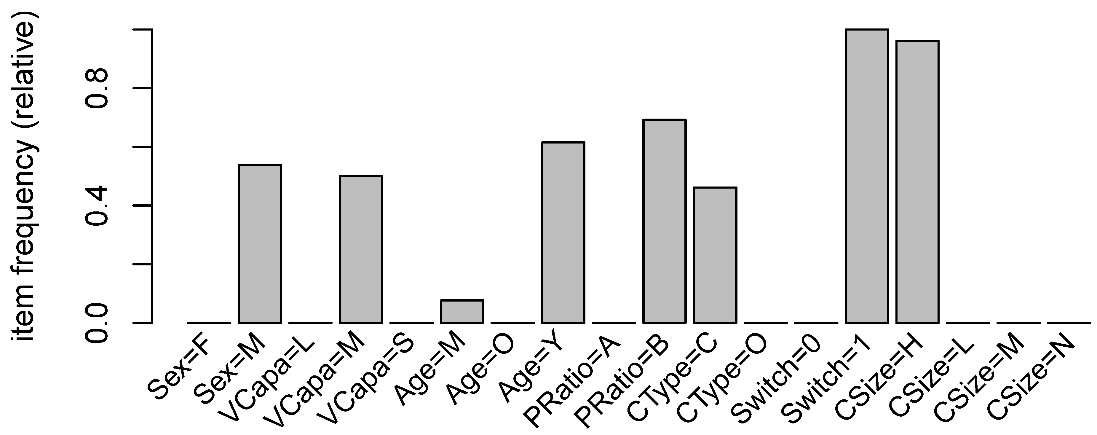
Our final dataset has a total of 893,009 observations of which 36.3% have a policy switch of 1.
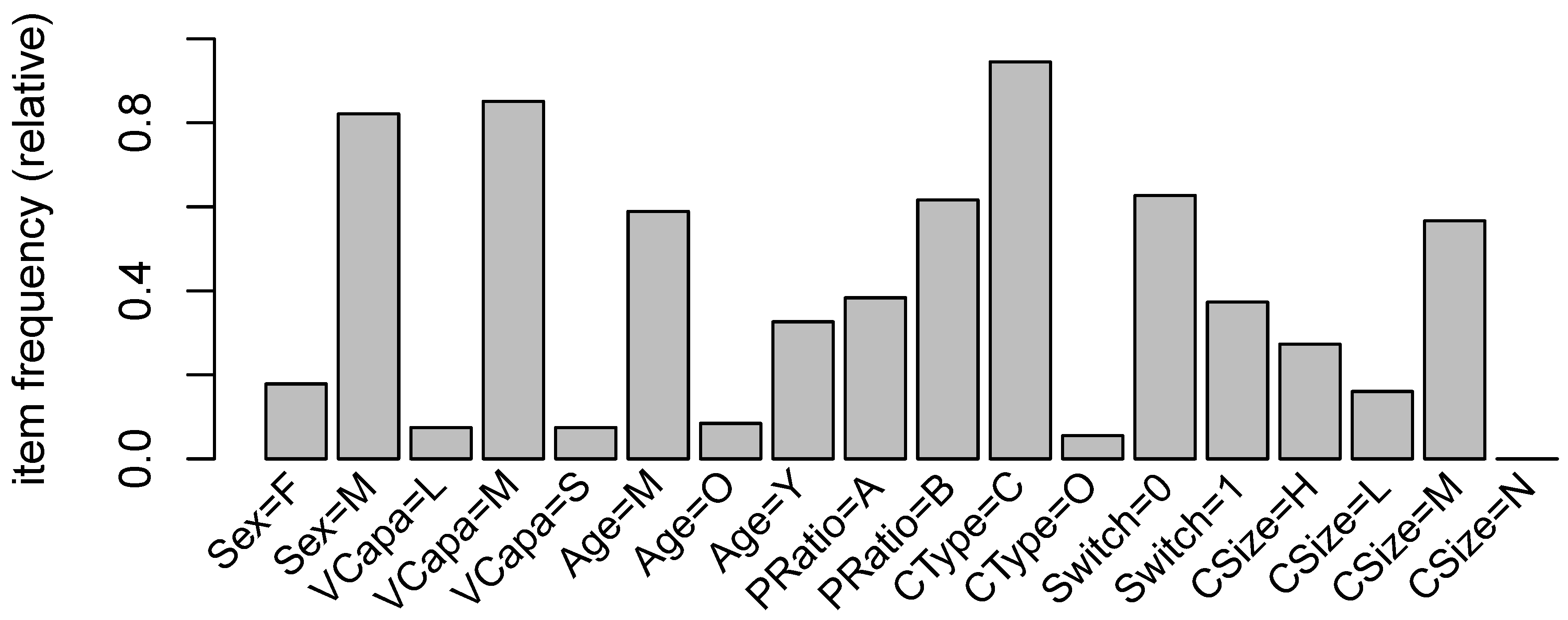
Figure 1 provides a graphical representation of the relative frequency of itemsets in our dataset.
Table 3 provides a list and description of the nine variables we used together with some simple summary statistics. The observations in our dataset consist of policies with comprehensive coverages for first party property damage and bodily injury as well as third party liability for property damage and bodily injury. The type of insurance coverage is predominantly Comprehensive with 82.9% of the total observations. The only vehicle characteristic that we can draw from our files is size or vehicle capacity, VCapa, defined to be the engine capacity measured in cubic centimeters (cc). We categorize the vehicles according to three categories of vehicle capacity: (Small, Medium, and Large). Most vehicles in our dataset are classified Medium size capacity, with about 82.5% of the total observations. We have gender and age that relate to driver information. More than 80% of the insured drivers are male and about two-thirds are in the middle age range. It is worth noting that due to gender equality issues, gender information is not allowed to be used in ratemaking according to European Union (EU) directives. Since our dataset was obtained from Singapore, we still keep the gender information in our analysis. Furthermore, some jurisdictions use gender for risk classification.
We categorize age according to whether Young (less than 35 years old), Middle (between 35 and 55 years old), and Old (55 years and older). It is worth noting that this categorization makes sense in Singapore. First, there is a very comprehensive public transportation system in Singapore so that driving at early age is not highly encouraged because of this convenience. Second, owning a vehicle in Singapore can be quite expensive and this is because of its size, the government controls the number of vehicles by imposing a large amount tax at purchase and for continued ownership. Finally, especially during the period of our observations, retirement was at about 55 years old, although it is likely that average retirement age today may have gone higher than this age.
The probability of having a claim is just as about what we expected: 11.8% of the observations had at least one claim during a calendar year. Of these observations with at least one claim, one-fifth had claim size below its first quartile (Low), two-thirds had claim size between the first and third quartile (Medium), and the rest had claim size above the third quartile (High). In order to relate premiums to claims and policy switch, we defined a variable called PremRatio which is equal to the ratio of the premium of this calendar year to that of the previous year. A PremRatio larger than one indicates in increase in premium while smaller than one indicates a decrease. We did some preliminary investigation as to what the suitable cutoff is for a premium ratio. Considering only those policies with claims, we find that the average rate of premium increase is 15% so that we considered any increase above this average to be AboveAvg and below this average to be BelowAvg. For any increase at exactly at 15%, this was considered BelowAvg. Of our total observations, 22.4% had premium increases that were above average. The choice of the premium rate increase was a reasonable one since we considered only those policies for which there was at least one claim. For many insurance companies, premium rate increase is not uncommon with or without a claim.
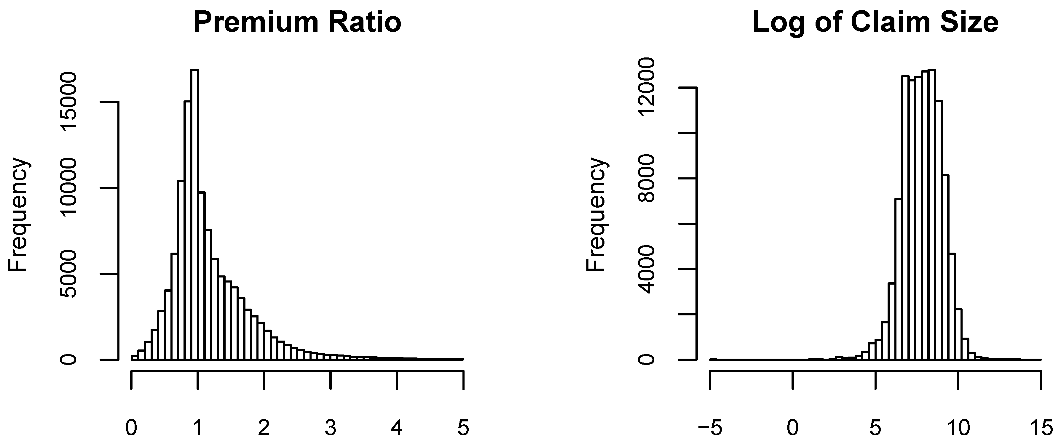
Figure 2 provides respective histograms of the premium ratio and the logarithm of the size of the claim, given the policy had a claim. The premium ratio variable has a minimum of 0.01 and a maximum of 4.99, with average of 1.17 and standard deviation of 0.6. Although we observe premium ratios as little as 0.01 and as large as 4.99, such extremes were not frequent in our dataset. Given the policy had a claim size, the size of the claim has a minimum of 0.01 and a maximum of 1,313,613 with average of and standard deviation of 11,179.56.
Table 4 provides additional statistics for these two variables describing the premium ratio and the size of the claim (in dollars). It is worth noting at this point that any reference to amounts here are in Singapore dollars.
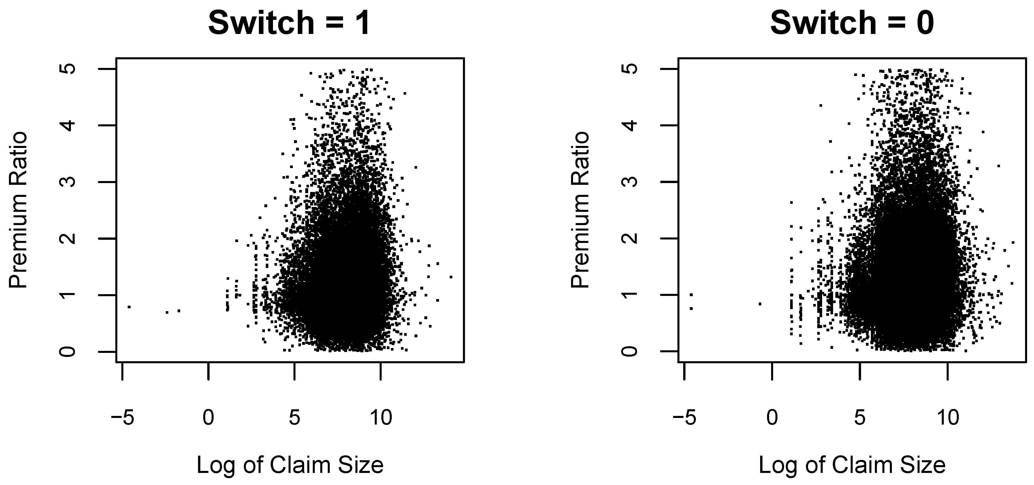
As we are simply interested in whether a policyholder switch is impacted by the size of the claim and the subsequent change in premium, we present
Figure 3 that provides the relationship between the size of claim (in logarithm) and the premium ratio according to whether there was a switch or not. According to this graphical evidence, we observe no relationship or pattern that we can observe. Traditional methods of supervised learning (e.g., generalized linear models) are less suitable in this regard. This is one of our motivation for using association rules to seek for evidence of policyholder lapse behavior according to the presence of a claim and the change in premium.
5. Concluding Remarks
In the insurance industry, there is increased interest in developing strategies for retaining policyholders even after a claim with little sacrifice for a lower profit margin. Policyholder retention have a positive effect on the company’s reputation for building good customer relationships which could further help attract new customers. It is well known that when experience rating is employed, a policyholder with at least one claim during a policy year will likely have an increase in premium in the subsequent policy year. Such is the core feature of an insurance market based on a bonus-malus system, that is, a policyholder is penalized after a claim. Depending on the level of premium increase, the policyholder may feel more likely to seek for another insurer willing to provide for a cheaper coverage. Sometimes, for example in the case of automobile insurance, a claim may change the driving behavior of the insured. Feeling the pressure of a further increase in premium, the driver may be more careful so that there is strong possibility of a better risk to the insurer. Insurers are therefore faced with the challenges of keeping premiums low, without too much sacrifice of profit margins, in order to retain policyholder loyalty. There has been no prior studies that provide for an empirical evidence of the possible association between policyholder switching after a claim and the associated change in premium. Using the method of association rule learning, a data mining technique that originated in marketing for analyzing and understanding consumer purchase behavior, we are able to provide evidence of such association in this article. This empirical investigation was made possible because of the unique dataset we have. We used a nine-year claims data for the entire Singapore automobile insurance market that allowed us to track information before and after a policy switch. Our results provide evidence of a strong association among the size of the claim, the level of premium increase, and policy switch. We attribute this to the possible inefficiency of the insurance market because of the lack of sharing and exchange of claims history among the companies. As possible future work, we would like to build predictive models to investigate the financial implications of such associations.


