Abstract
Stochastic mortality models have been developed for a range of applications from demographic projections to financial management. Financial risk based models built on methods used for interest rates and apply these to mortality rates. They have the advantage of being applied to financial pricing and the management of longevity risk. Olivier and Jeffery (2004) and Smith (2005) proposed a model based on a forward-rate mortality framework with stochastic factors driven by univariate gamma random variables irrespective of age or duration. We assess and further develop this model. We generalize random shocks from a univariate gamma to a univariate Tweedie distribution and allow for the distributions to vary by age. Furthermore, since dependence between ages is an observed characteristic of mortality rate improvements, we formulate a multivariate framework using copulas. We find that dependence increases with age and introduce a suitable covariance structure, one that is related to the notion of ax minimum. The resulting model provides a more realistic basis for capturing the risk of mortality improvements and serves to enhance longevity risk management for pension and insurance funds.
1. Introduction
A variety of empirical studies across many developed nations show that mortality trends have been improving stochastically; see, e.g., CMI (2005), Luciano and Vigna (2005), Blake et al. (2006), Liu (2008) and Blackburn and Sherris (2013). Numerous stochastic mortality models proposed in the literature apply extensions of interest rate term structure modelling, known as short-rate models. In particular, the Cox–Ingersoll–Ross (CIR) model, Cox et al. (1985), has been adapted in Luciano and Vigna (2005), who use a time inhomogeneous version of the process to model the mortality dynamics. Furthermore, Biffis (2005), Russo et al. (2010) and Blackburn and Sherris (2013) develop a variety of affine frameworks extended from interest rate term structure modelling. Blake et al. (2006), Cairns et al. (2006), Bauer (2006) and Bauer and Ruß (2006) demonstrate that, if mortality risk can be traded through securities such as longevity bonds and swaps, then the techniques developed in financial markets for pricing bonds and swaps can be adapted for mortality risk. Such models have the advantage of being able to incorporate a price of longevity risk and have applications to the valuation of mortality linked contracts, which can be used to mitigate longevity risk on life insurance products, including annuities. A typical underlying assumption in these models is that mortality rates are Gaussian.
An alternative to short-rate models is provided by forward-rate approaches that model forward forces of mortality and forward survival probabilities. Olivier and Jeffery (2004) and Smith (2005) apply a forward-rate mortality framework with stochastic factors driven by univariate gamma random variables irrespective of age or duration. Although the model is conceptually interesting, not much has been done to assess the validity of the model assumptions. In addition to restricting the stochastic factors to identical gamma distributions, another critical assumption is that of independence amongst these factors across age. We examine these assumptions using England and Wales female mortality data for 1960 to 2009; a dataset used in Cairns (2007).
Based on the empirical analysis, we generalize the Olivier–Smith model in order to provide a more realistic basis for capturing the risk of mortality improvements. Previous studies, e.g., Wills and Sherris (2010) and Jevtić et al. (2013), have verified that dependence plays a critical role in mortality modelling. A more realistic risk factor structure that captures such features of mortality data has the potential to provide enhanced risk management techniques for mitigating the longevity risk faced by pension funds and annuity providers.
We assume random shocks are driven by non-identical univariate Tweedie random variables. By specifying the Tweedie distribution, we incorporate the Gaussian, compound Poisson, gamma and inverse Gaussian distributions, which are all characterised by a power variance function; the Tweedie distribution has been widely adopted in actuarial science, see, e.g., Aalen (1992), Jørgensen and De Souza (1994), Kaas (2005) and Furman and Landsman (2010). We, thereby, allow the stochastic components to originate from distributions with varying levels of volatility. Rather than to generalise further to the exponential dispersion family, we presently restrict our attention to the Tweedie distribution due to the convenient form of the cumulant function, which leads to straightforward implementation. Our empirical investigations show this to be highly desirable. Furthermore, by specifying the Tweedie distribution, we can readily incorporate a relevant set of marginal distributions. We test both the Gaussian and gamma distributions and provide evidence that the gamma is the more suitable of the two. Since dependence between ages is an observed characteristic of mortality rate improvements, we further generalize the model by formulating a multivariate distribution that incorporates age dependence using copulas. In order to accomplish this, we introduce a new covariance pattern, one that is governed by the minimum of the two age covariates. That is, the correlation between mortality rates of two ages depends only on the least of the two; this notion is applied to the age range 49–99.
In Section 2, we introduce the necessary notation, providing background context for the forward- rate mortality framework, and describe the Olivier–Smith model. We assess the model using data from England and Wales in Section 3. In Section 2.3, we introduce a univariate Tweedie generalization and, in Section 4, consider a multivariate framework using copulas. Section 5 concludes the paper.
2. Forward Mortality Framework
Before providing the Olivier–Smith model and a straightforward univariate generalization, we provide a revision of longevity bonds and their forward price. We note that Section 2.1 provides contextual background information.
2.1. Longevity Bond Pricing
Let denote the short rate at time t, and let be the cash account defined as
Let , the discount bond price, denote the value at time t of receiving 1 at time T:
where is the risk neutral probability measure derived from observable market prices and represents the available information at time t—in this case, the evolution of the short rate process until time t is relevant. The discount bond price can also be expressed in terms of forward rates, namely
where is the instantaneous rate of interest at time implied by the interest rate market at time t; i.e., the forward interest rate. The discount bond price represents a current value (time t) using current information (). In general, we might be interested in the future value (say, at time ) of receiving 1 at future time (time ) using current information (); for which we use the notation :
Thereby, we assume independent increments of the interest rate process. In the context of derivatives, is the forward price of a -maturity bond at .
Let denote the force of mortality at time t for age . This implies that x is the age at time zero. The age-specific survivor index is given by
The survivor index is the probability an individual aged x at time zero survives to time t. Notice the similarities of the cash account and the survivor index. Both are based on an instantaneous process. In the case of the cash account, the short rate; in the case of the survivor index, the force of mortality. However, unlike the short rate, the force of mortality also includes an age component. Clearly, ; with the restriction of negative interest rates and forces of mortality, we have that the cash account increases and the survivor index decreases.
Now, consider a refinement of that incorporates mortality, denote it , the longevity bond. Rather than paying 1 at time T, it pays , representative of the proportion of survivors. For example, suppose one is liable to pay 1 at time T to the survivors of a group of individuals, all of whom are aged x at time zero. Ignoring basis risk, the longevity bond represents a perfect hedging instrument. The price of the longevity bond is given by
where is the risk neutral probability measure derived from observable market prices and represents the available information at time t—in this case, both the evolution of the short rate and mortality processes until time t are relevant.
As before, we can rewrite using forward rates. Our aim is to study mortality rates in isolation, rather than in conjunction with interest rates, and so, we presently assume the two are independent:
where is the instantaneous mortality rate at time for age implied by the longevity bond market at time t; i.e., the forward mortality rate. Again, we can generalize to the forward price of the longevity bond to obtain
where represents the forward price of the mortality-component of a -maturity longevity bond at time ; it is given by
Here, similarly to the interest rate process, we assume independent increments of the mortality process. Notice, therefore, that forward prices are multiplicative in the sense that the duration can be compartmentalized; for example, we have that
It is clear that the above results depend entirely on the existence of an arbitrage-free market, which, unfortunately, is not the case. Therefore, as pointed out in Norberg (2010), the application of risk-neutral pricing is called into question. It is not our intention to enter this debate, rather to demonstrate the results under these principles and further encourage the emergence of a longevity bond market.
Presently, we assume that the market price of longevity risk is constant, and, for convenience, zero; this has previously been done in, e.g., in Ziveyi et al. (2013) and Ignatieva et al. (2018) in relation to the pricing of life insurance products. The result of this work would not be impacted if arbitrary were selected to represent the market price of longevity risk, since it is true that, in practice, investors will certainly demand a risk premium. However, as our interest lies in assessing volatility, not drift, setting does not represent an issue and is done for convenience. Consequently, we have that p, the mortality forward price, is also the expected future mortality spot price:
In other words, is the expected probability an individual age x at time zero survives to time given survival to time , based on available information ; it is an expected forward conditional survival probability.
Finally, the requirement of the martingale property implies
2.2. The Olivier–Smith Model
Rather than suppose a structure for the mortality rate process, volatility can also be imposed directly via the forward rates with random shocks. This was proposed in the Olivier–Smith model given below; see Olivier and Jeffery (2004), Smith (2005).
Model 1.
For all ages x and forward-times
whereare independent and identically distributed gamma random variables with shape and rate parameter, such thatand. Furthermore, theare-measurable bias correction functions given by
For an arbitrage-free market, we require the martingale property, that is, Equation (1) to be satisfied. Consequently, we obtain
see, e.g., Cairns (2007) for the details of this derivation, which rests on standard properties of the gamma distribution and the use of moment generating functions.
The model restricts the stochastic nature of mortality evolution by imposing gamma, , random variables.
2.3. Univariate Tweedie Generalization
We briefly introduce the Tweedie distribution, first formulated in Tweedie (1984); also see McCullagh and Nelder (1989).
Let denote a random variable belonging to the additive exponential dispersion family (EDF) with probability measure , absolutely continuous with respect to ,
where is called the cumulant; see Jørgensen (1997), Section 3.1. The parameters and are called the canonical and dispersion parameter, respectively, is a twice differentiable function, and the expectation of X is given by
Furthermore, is a one-to-one map and there exists an inverse function
The function is called the unit variance function. The Tweedie subclass, denoted , is the class of EDF with power unit variance function
where p is called the power parameter. The values correspond to the normal, over-dispersed Poisson, gamma, and inverse Gaussian distributions, respectively. The cumulant has the form
where .
Model 2.
For all ages x and forward-times
whereare independent and identically distributed Tweedie random variables,withand. Furthermore, theare-measurable bias correction functions given by
For an arbitrage-free market, we require the martingale property, that is, Equation (1) to be satisfied. Consequently, we obtain
where
is the moment generating function of . This reduces to the Olivier–Smith model if we select , , and .
The b functions are derived following a recursive procedure. First, we investigate the case with a maturity of . From the above, we have
which yields
From this, it is clear that
Substracting the two equations from one another leaves
Note that , consequently, the expression above holds for the case with maturity . Therefore, this is the general expression and we no longer require the recursive argument.
Henceforth, we generalize the stochastic component and, instead, make use of the notation :
3. Model Assessment
The Olivier–Smith model makes two main assumptions regarding the stochastic mortality component. The first is that of a gamma distribution. The second is that the distribution that generates the components does not depend on time t; that is, that mortality components are identically distributed. The Olivier–Smith model was not intended for multiple cohorts. However, it is our desire to apply the model to multiple cohorts, and so we begin by assuming the mortality components are also independent across cohorts. Combined, this means that the components are assumed to be independent and identically distributed. We presently investigate the validity of these assumptions (the first two specified by the Olivier–Smith model, whereas the latter is our own) using real data. We assume and treat population mortality rates as risk neutral.
In a risk neutral framework with constant annual forces of mortality and one-year forward rates, we have, for all t, all x, and ,
where is the maximum attainable age. Notice that the above formulation of the forward rate does not include any imposed improvement trend. That is, the forward mortality probability for an individual aged x in T years is taken from an individual presently aged . We recognize that this may be seen as rather controversial. Our justification for the above equation is that we believe any inclusion of trend would largely be a part of bias correction functions b and only have a minor influence on the volatility. Again, since our aim is to investigate the behaviour of the mortality components Z, rather than trends, we feel justified in our approach. We do not claim that this is the only way in which to proceed; however, we feel it is an avenue worthy of exploration.
Consequently, keeping the above in mind, we define for all t, all x, and ,
We use female central mortality rates from the Human Mortality Database (2013) for England and Wales Total Population for the period 1960–2009, and ages 0–105 (). We extract observations of from the data. England and Wales data were selected since it is a commonly used benchmark dataset.
3.1. Independent Distributions
In this section, we investigate whether the stochastic components are independent. We address this in two ways: by considering the linear correlation structure between appropriately selected sub-samples, and applying a principal component analysis.
3.1.1. Correlation Analysis
We explore the correlation structure between the stochastic mortality components over time and forward-age. Figure 1 suggests no particular dependence pattern over time; roughly 90% of the correlations have absolute value less than 0.35. That is, the collection of observations of the stochastic component from calendar year s appear uncorrelated with the collection from calendar year . This is evidence of independence over the time dimension.
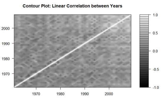
Figure 1.
Correlations of and .
Figure 2 provides contour plots of correlation between the stochastic components over forward-age. In contrast to the contour plots over time, we do notice varying levels of correlation over forward-age, especially amongst the older ages. The correlation appears very volatile for the younger forward-ages. This is a technical consequence of having comparatively smaller sample sizes for forward-ages 0–48. Furthermore, correlation patterns are difficult to discern when centenarians are included. This is related to the high volatility of mortality data for centenarians. Consequently, we provide the contour plot for ages 49–99 in the second panel of Figure 2. Lighter shades of gray indicate higher positive correlation; the plot provides clear evidence that correlation increases with forward-age.
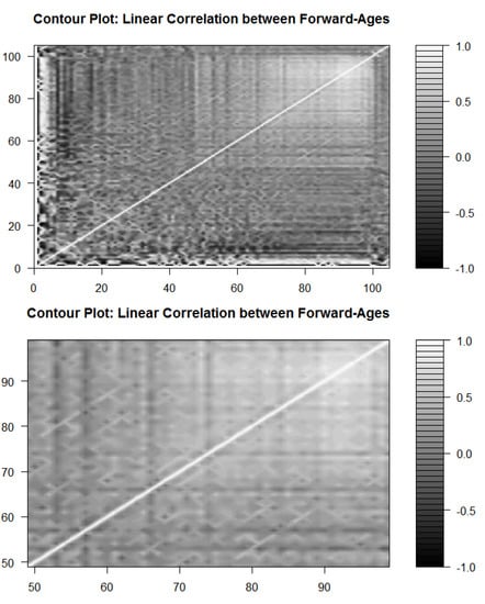
Figure 2.
Correlations of and .
3.1.2. Principal Component Analysis
In the previous section, we found evidence that the stochastic mortality components are correlated by forward-age, which is especially pronounced for the older ages. In order to further investigate this form of dependence, we perform a principal component analysis (PCA) for the random components taken with respect to different forward-ages. We focus on forward-ages 49–99; represented in the second panel of Figure 2. Therefore, with 49 years of observations, we obtain a 51 by 49 matrix of stochastic components by forward-age and time.
PCA is applied to multivariate data in order to take advantage of possible redundancy due to dependence. By using linear combinations of the original variables, we transform the 51 correlated variables (stochastic components by forward-ages) into uncorrelated ones of a lower dimension. In general, PCA may either be applied to the covariance, or correlation matrix. PCA applied to the correlation matrix is typically used when variables are measured in different units. Since this is not the case in our data, we elect to apply PCA to the covariance matrix. In addition, standardising produces data with the same variation. This is not desirable since we want to preserve differences in variation by forward-age.
Table 1 summarises the results of the PCA applied to the covariance matrix. Note that, as a criteria for deciding on the number of components, one typically chooses the number of components that cumulatively account for a meaningful percentage of the variance (typically around 70%). We select the first 4 components since they account for approximately 74% of the variance; see Table 1.

Table 1.
PCA results.
Figure 3 shows the top four principal components. They represent key movement in the random component by forward-age. We observe that some factors affect the stochastic components irrespective of forward-age, while others affect stochastic components from younger and older forward-ages quite differently. For example, the first principal component, which explains approximately 28% of the variation, exhibits a clear upward trend. This indicates that stochastic components from older forward-ages are more influenced than those from lower forward-ages. This confirms the result from Figure 2 that correlation increases by forward-age. Although the third and fourth principal components exhibit a downward trend, they are of less significance since they collectively account for less than 25% of the variance.
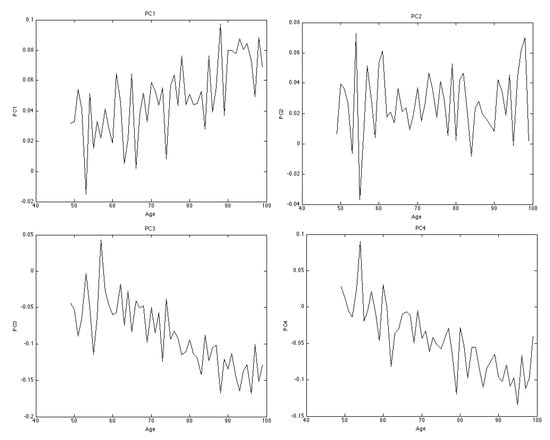
Figure 3.
Top four principal components.
Finally, the biplots in Figure 4 show the magnitude and sign of each variable’s contribution to the first two (upper panel) or three (lower panel) principal components, and how each observation is represented in terms of those components. The axes in the plot represent the principal components, the coefficients of the variables (forward-ages) on the principal components are represented as vectors, and the points are the scores of the observations (years) on the principal components.
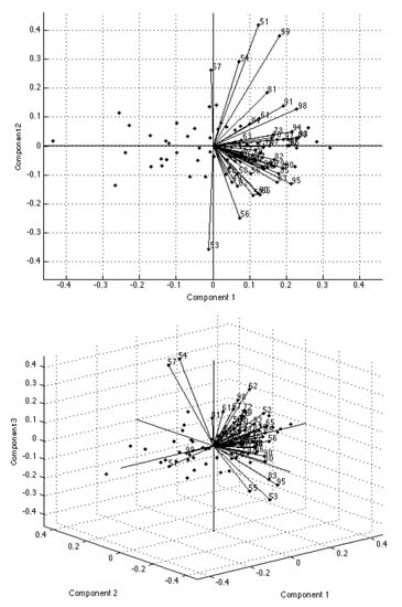
Figure 4.
Biplots of the principal components.
Both the empirical investigation and the PCA provide evidence of correlation between the stochastic mortality components, especially among the older ages. The assumption of independent distributions for the stochastic mortality component is therefore violated.
3.2. Identical Distributions
In this section, we investigate whether the stochastic mortality components come from identical distributions. Although we have identified potential dependence over forward-age, it is not conclusive, and, therefore, we also investigate plots of the stochastic component over this dimension.
Figure 5 shows the observations of Z over time t for various fixed combinations of T and x. Over time t, the Z resembles a random sample. However, the underlying distribution changes with respect to the forward-age, , of the mortality components. The scale of the first plot is roughly five times larger than the others. This implies that the first plot demonstrates very high volatility, which is not surprising given that this plot represents a forward-age of 105.
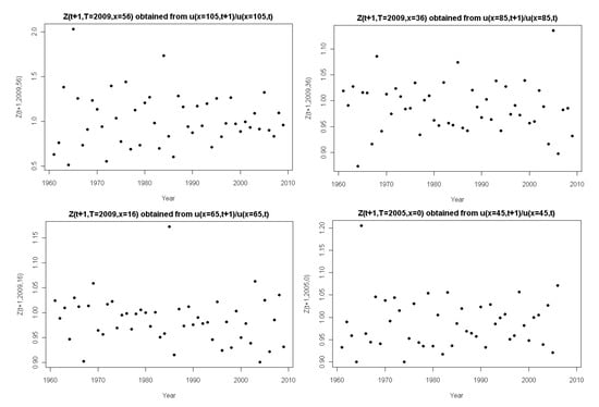
Figure 5.
The stochastic mortality component over time t for fixed x.
Figure 6 shows the observations of Z over age x for various fixed t. Recall that we have no observations of Z for ; for , we obtain a similar plot as that of , where the only difference is a shift in the x-axis, representative of a translation of the forward-age. We present the plots for as they are most informative. Figure 6 reinforces what is observed in Figure 5. The volatility of the stochastic component clearly varies with age. The forward-ages 0–40 and 90 plus generally exhibiting high volatility, with the remaining forward-ages, 40–90, exhibiting comparatively lower volatility.
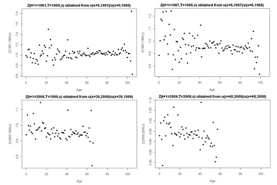
Figure 6.
The stochastic mortality component over age x for fixed t.
In Figure 7, we fix the year-of-birth and plot over time, which is representative of tracking a single cohort. We notice that volatility varies with forward-age, which is visible to a greater or lesser extent depending on which forward-age-range the cohort traverses; notice the different scales of the plots in this figure. However, given the contour plots in Section 3.1, the samples in Figure 7 most likely violate the independence assumption. Therefore, caution must be exercised when interpreting these plots. Figure 6 and Figure 7 provide evidence that the volatility of the stochastic component are not homogeneous over forward-ages. The assumption of identical distributions for the stochastic mortality component is therefore violated.
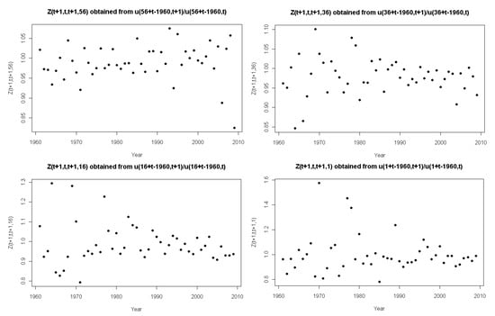
Figure 7.
The stochastic mortality component for fixed year-of-birth.
3.3. Appropriate Parametric Distribution
From the data shown in Figure 5, Figure 6 and Figure 7, it is difficult to conclude whether the gamma distribution provides a good fit to the data. Fitting the data presumes independent and identically distributed observations, both of which may be violated.
However, we present quantile-to-quantile (QQ) plots and formal distributional (goodness-of-fit) tests to investigate the suitability of the gamma distribution. Figure 8, Figure 9 and Figure 10 show the QQ plots corresponding to Figure 5, Figure 6 and Figure 7, respectively. They contrast the quantiles of the empirical distribution with those from the estimated gamma distribution. A deviation from the 45 degree line indicates a departure from the assumed distribution. The results indicate the gamma distribution provides a reasonable fit for the stochastic mortality component over time t; see Figure 8. Figure 9 and Figure 10 are less relevant, since they represent fitting the distribution over age and year-of-birth, respectively, where we have evidence that the independent and identical distribution assumption is violated. This means that the lack in fit is not very informative.
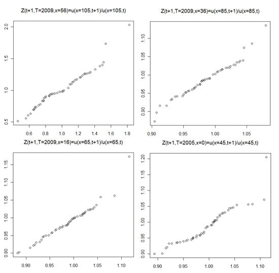
Figure 8.
The stochastic mortality component over time t for fixed x; quantile-to-quantile (QQ) plot corresponding to Figure 5.
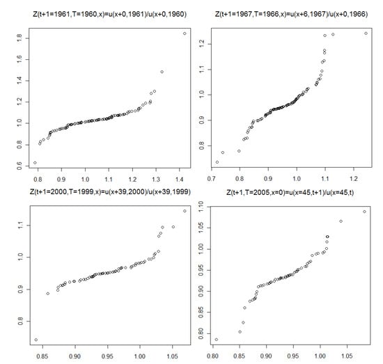
Figure 9.
The stochastic mortality component over age x for fixed t; QQ plot corresponding to Figure 6.
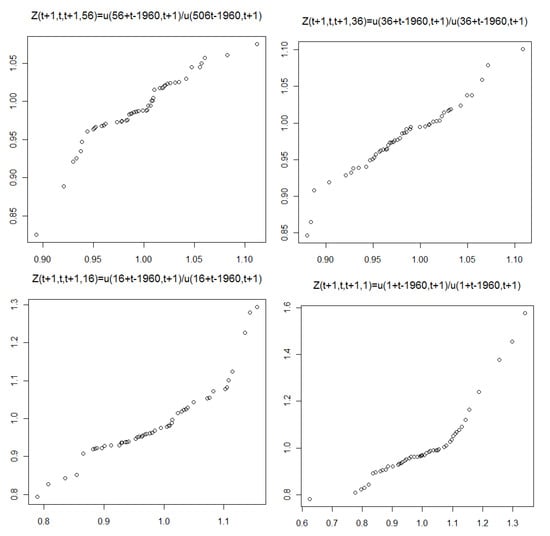
Figure 10.
The stochastic mortality component for fixed year-of-birth; QQ plot corresponding to Figure 7.
We apply the goodness-of-fit tests suggested in D’Agostino and Stephens (1986) and Stephens (1974). We test the null hypothesis that the data belongs to the theoretical (hypothesized) gamma distribution, that is, , where represents the empirical cumulative distribution function (cdf) and , the theoretical cdf with estimated parameters obtained from maximum likelihood. Let the be ordered observations, and , the resulting estimated quantiles. We consider the following test statistics:
- The Anderson–Darling statistic , given by
- The Kolmogorov statistic D, given by , whereThe modified form statistic proposed in Stephens (1974) together with the critical values corresponds to .
- The Cramér–von Mises statistic , given byThe modified form statistic reported in Stephens (1974) is given by .
The critical values for the above tests are specified in Table 2, as provided in D’Agostino and Stephens (1986) and Stephens (1974).
Table 2.
Critical values for the goodness-of-fit tests.
Table 3 summarizes the results for the goodness-of-fit tests; * and ** indicate the gamma assumption is not rejected at a and significance level, respectively, where the gamma density is given by
Table 3.
Distributional test results.
The distributional tests confirm the results observed from the QQ plots. The gamma distribution is not rejected at either significance level for the observations of stochastic mortality component over time (Panel A). The results for stochastic mortality component over age for fixed calendar year (Panel B) and over time for fixed year-of-birth (Panel C) are mixed. Again, the mixed results in Panel B and C are likely due to the violation of the independent and identical distribution assumption of these samples. Finally, note from Table 3 that the estimates of the shape and rate parameters, and , are approximately equal, which confirms the assumption that the expected value of the stochastic component is one.
4. Multivariate Generalization
We begin by formulating the most general model.
Model 3.
For all ages x and forward-times
where Z follows any multivariate distribution. Theare some-measurable bias correction functions.
To preserve the martingale property, we have
To proceed further, a multivariate distribution must be specified for the Z. We do so using copulas. Copulas provide the means to effectively study any form of dependence; see, e.g., Embrechts et al. (2002), Breymann et al. (2003), and McNeil et al. (2005). We focus on the use of the elliptical family. Previous work modelling dependence using the elliptical family include Hult and Lindskog (2002), Fang et al. (2002), and Frahm et al. (2003). Figure 2 suggests that the correlation between any pair of stochastic components depends on the smallest of the two associated forward-ages. This produces the “L” shapes intersecting the diagonal of the plot; see Figure 2 above. To accommodate this form of dependence, we introduce the minimum covariance pattern.
4.1. Minimum Covariance Pattern
The minimum covariance pattern makes the assumption that the correlation between any pair of responses is determined solely by the minimum value of the corresponding covariate; in this case, forward-age. That is, . Note that this results in correlation parameters:
4.2. Capturing Dependence with Copulas
Copulas are multivariate distribution functions relating d one-dimensional standard uniform marginals to a joint distribution. If F is a d-dimensional distribution function with marginals , then, for every , there exists a copula C with
Equivalently, if C is a copula and are distribution functions, then the function F defined above is a joint distribution function with marginals . If are continuous, then C is unique. Thus, if is a random vector with distribution and continuous marginals , then the copula of X is the distribution function of , where :
The above formulation is found in Sklar’s Theorem; see Joe (1997) for a proof.
Two scatter-plots shown in Figure 11 highlight the different levels of dependence between observations from younger versus older forward-ages. We investigated the scatter-plots originating from observations of all possible pairs of forward-ages and found no evidence of non-standard types of dependence. Therefore, we consider the Gaussian copula. In order to allow for the presence of tail-dependence, we also consider the Student’s t copula. We note that other copulas, including those generating asymmetric tail dependence, would be interesting to consider; we leave this for future research.
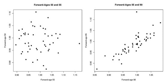
Figure 11.
Scatter plots for observations by forward-age.
With respect to the marginals, we consider both the gamma and the Gaussian distributions. The gamma distribution because it was originally considered in the Olivier–Smith model; we choose to compare it with the Gaussian distribution since it is the most widely used member of the Tweedie family. The Gaussian distribution was also considered in Olivier and Jeffery (2004). They claimed results similar to the gamma distribution, although no formal analysis was provided.
The literature suggests various approaches to estimate copulas; see, e.g., Joe (1997) and Cherubini et al. (2004). We make use of the so-called inference for marginals (IFM) method, which is a sequential two-step maximum likelihood approach. First, one estimates the marginal parameters; subsequently, the copula to obtain the pseudo log-likelihood function, which is then maximized with respect to the copula dependence parameter. For details on the IFM and alternative estimation techniques, see MacLeish and Small (1988) and Joe (1997).
The minimum covariance pattern described above is not implemented in any statistical packages we are aware of. Therefore, we fit the Gaussian and Student’s t copulas with an unstructured correlation matrix, given below:
Using the output, , we construct the parameter estimates from the minimum covariance pattern as follows:
The ability to specify the minimum covariance pattern would enhance estimation. Figure 12 shows the estimation of the correlation parameters for the Gaussian copula with gamma marginal distributions in the unstructured and minimum covariance patterns. The similarities between the two contour plots confirm that the minimum covariance pattern is suitable in this case. Figure 13 shows the equivalent using the Student’s t copula.
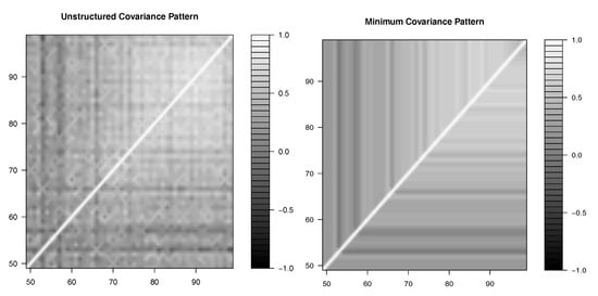
Figure 12.
Contour plots for the Gaussian copula.
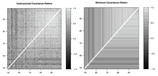
Figure 13.
Contour plots for the Student’s t copula.
Figure 14 shows the estimated variance of the gamma marginal distributions by forward-age. A very similar result is produced under the assumption of Gaussian marginals. The fluctuations in the variance clearly demonstrate that the marginal distributions vary by forward-age.
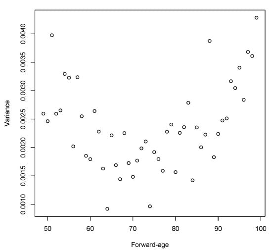
Figure 14.
Variance estimation.
To produce the contour plots and the variance plot (Figure 12, Figure 13 and Figure 14), we make use of the inversion of Kendall’s tau method developed in Joe (1990). This was done because likelihood-based methods cannot readily estimate 51-dimensional copulas.
Finally, to examine the performance of the considered copula models, we use the Akaike Information Criterion (AIC) introduced in Akaike (1974):
where denotes the maximized value of the log-likelihood and q the number of estimated parameters. Smaller values of AIC indicate a better fit.
We compute the AIC for groups of forward-ages, as summarized in the first column of Table 4. We split the sample into five sub-samples of 11 forward-ages in order to overcome the dimensionality issue arising when fitting a 51-dimensional copula using the likelihood-based IFM method. The Gaussian copula outperforms the Student’s t copula for forward-ages up to 79, and under-performs for forward-ages above 79. This provides evidence of tail-dependence at the older forward-ages. With respect to the marginal distributions, the gamma consistently outperforms the Gaussian distribution. Since many models rely on Gaussian marginals, the result that the gamma outperforms the Gaussian distribution is rather significant. The fact that the gamma distribution outperforms the Gaussian distribution may lead some to thinking that the generalisation is overcomplicated rather than necessary, but, in fact, this conclusion rests on the existence of the generalisation in the first place, thereby confirming its value. The fact that the modelling framework advocated in this paper allows for this added flexibility in the choice of marginal distributions is shown to be a very desirable attribute.
Table 4.
Model comparison (Akaike Information Criterion).
5. Conclusions
We investigate the Olivier–Smith model and show that, using population mortality data for England and Wales, the model requires a more general framework, with additional emphasis on age dependence and marginal distributions that vary by forward-age. The gamma distribution provides a reasonable fit, but is a restrictive assumption. We improve the model by specifying a more general distribution, namely the Tweedie class of the exponential dispersion family. In addition to allowing the distribution to vary by forward-age, we also incorporate dependence between forward-ages using copulas. To accommodate the nature of the dependence, we specify a new covariance pattern related to the notion of minimum.
Author Contributions
Methodology and formal analysis, D.H.A., K.I. and M.S.; software, D.H.A. and K.I.; writing (original draft and editing), D.H.A., K.I. and M.S.; projet administration, M.S.
Funding
This research was funded by ARC Linkage Grant Project LP0883398 Managing Risk with Insurance and Superannuation as Individuals Age with industry partners PwC, APRA and the World Bank as well as the support of the Australian Research Council Centre of Excellence in Population Ageing Research (project number CE110001029).
Conflicts of Interest
The authors declare no conflict of interest.
References
- Aalen, Odd O. 1992. Modelling heterogeneity in survival analysis by the compound Poisson distribution. Annals of Applied Probability 2: 951–72. [Google Scholar] [CrossRef]
- Akaike, Hirotugu. 1974. A new look at the statistical model identification. IEEE Transaction on Automatic Control 19: 716–23. [Google Scholar] [CrossRef]
- Bauer, Daniel. 2006. An Arbitrage-Free Family of Longevity Bonds. Ulm: University of Ulm. [Google Scholar]
- Bauer, Daniel, and Jochen Ruß. 2006. Pricing longevity bonds using implied survival probabilities. Paper presented at Meeting of the American Risk and Insurance Association (ARIA), Washington, DC, USA, August 6. [Google Scholar]
- Biffis, Enrico. 2005. Affine processes for dynamic mortality and actuarial valuations. Insurance: Mathematics and Economics 37: 443–68. [Google Scholar] [CrossRef]
- Blackburn, Craig, and Michael Sherris. 2013. Consistent dynamic affine mortality models for longevity risk applications. Insurance: Mathematics and Economics 53: 64–73. [Google Scholar] [CrossRef]
- Blake, David, Andrew J. G. Cairns, and Kevin Dowd. 2006. Living with mortality: Longevity bonds and other mortality-linked securities. British Actuarial Journal 12: 153–97. [Google Scholar] [CrossRef]
- Breymann, Wolfgang, Alexandra Dias, and Paul Embrechts. 2003. Dependence structures for multivariate high-frequency data in finance. Quantitative Finance 3: 1–14. [Google Scholar] [CrossRef]
- Cairns, Andrew J. G. 2007. A multifactor generalisation of the Olivier-Smith model for stochastic mortality. Paper presented at 1st IAA Life Colloquium, Stockholm, Sweden, June 10–13. [Google Scholar]
- Cairns, Andrew J. G., David Blake, and Kevin Dowd. 2006. Pricing death: Frameworks for the valuation and securitization of mortality risk. ASTIN Bulletin 36: 79–120. [Google Scholar] [CrossRef]
- Cherubini, Umberto, Elisa Luciano, and Walter Vecchiato. 2004. Copula Methods in Finance. Hoboken: Wiley Finance Series. [Google Scholar]
- CMI. 2005. Projecting Future Mortality: Towards a Proposal for a Stochastic Methodology. Working Paper 15 of the Continuous Mortality Investigation. London: The Faculty of Actuaries and Institute of Actuaries. [Google Scholar]
- Cox, John C., Jonathan E. Ingersoll, Jr., and Stephen A. Ross. 1985. A theory of the term structure of interest rates. Econometrica: Journal of the Econometric Society 53: 385–407. [Google Scholar] [CrossRef]
- D’Agostino, Ralph B., and Michael A. Stephens. 1986. Goodness-of-fit techniques. In Statistics: Textbooks and Monographs. New York: Dekker. [Google Scholar]
- Embrechts, Paul, Alexander McNeil, and Daniel Straumann. 2002. Correlation and dependence in risk management: Properties and pitfalls. In Risk Management: Value at Risk and Beyond. Cambridge: Cambridge University Press, pp. 176–223. [Google Scholar]
- Fang, Hong-Bin, Kai-Tai Fang, and Samuel Kotz. 2002. The meta-elliptical distributions with given marginals. Journal of Multivariate Analysis 82: 1–16. [Google Scholar] [CrossRef]
- Frahm, Gabriel, Markus Junker, and Alexander Szimayer. 2003. Elliptical copulas: Applicability and limitations. Statistics and Probability Letters 63: 275–86. [Google Scholar] [CrossRef]
- Furman, Edward, and Zinoviy Landsman. 2010. Multivariate Tweedie distributions and some related capital-at-risk analysis. Insurance: Mathematics and Economics 46: 351–61. [Google Scholar]
- Hult, Henrik, and Filip Lindskog. 2002. Multivariate extremes, aggregation and dependence in elliptical distributions. Advances in Applied Probability 34: 587–608. [Google Scholar] [CrossRef]
- Human Mortality Database. 2013. University of California, Berkeley (USA), and Max Planck Institute for Demographic Research (Germany). Available online: www.mortality.org or www.humanmortality.de (accessed on 8 March 2013).
- Ignatieva, Katja, Andrew Song, and Jonathan Ziveyi. 2018. Fourier space time-stepping algorithm for valuing guaranteed minimum withdrawal benefits in variable annuities under regime-switching and stochastic mortality. ASTIN Bulletin 48: 139–69. [Google Scholar] [CrossRef]
- Jevtić, Petar, Elisa Luciano, and Elena Vigna. 2013. Mortality surface by means of continuous time cohort models. Insurance: Mathematics and Economics 53: 122–33. [Google Scholar] [CrossRef]
- Joe, Harry. 1990. Multivariate concordance. Journal of Multivariate Analysis 35: 12–30. [Google Scholar] [CrossRef]
- Joe, Harry. 1997. Multivariate Models and Dependence Concepts. London: Chapman & Hall. [Google Scholar]
- Jørgensen, Bent. 1997. The Theory of Dispersion Models. London: Chapman & Hall. [Google Scholar]
- Jørgensen, Bent, and Marta C. Paes De Souza. 1994. Fitting Tweedie’s compound Poisson model to insurance claims data. Scandinavian Actuarial Journal 1: 69–93. [Google Scholar] [CrossRef]
- Kaas, Rob. 2005. Compound Poisson Distributions and GLM’s—Tweedie’s Distribution. Brussels: Royal Flemish Academy of Belgium for Science and the Arts. [Google Scholar]
- Liu, Xiaoming. 2008. Stochastic Mortality Modelling. Ph.D. thesis, University of Toronto, Toronto, ON, Canada. [Google Scholar]
- Luciano, Elisa, and Elena Vigna. 2005. Non Mean Reverting Affine Processes for Stochastic Mortality. Torino: International Centre for Economic Research. [Google Scholar]
- MacLeish, Donald L., and Christopher G. Small. 1988. The Theory and Applications of Statistical Inference Functions. New York: Springer. [Google Scholar]
- McCullagh, Peter, and John A. Nelder. 1989. Generalized Linear Models, 2nd ed. London: Chapman & Hall. [Google Scholar]
- McNeil, Alexander J., Rüdiger Frey, and Paul Embrechts. 2005. Quantitative Risk Management. Princeton: Princeton Series in Finance. [Google Scholar]
- Norberg, Ragnar. 2010. Forward mortality and other vital rates—Are they the way forward? Insurance: Mathematics and Economics 47: 105–12. [Google Scholar] [CrossRef]
- Olivier, Phillip, and Tony Jeffery. 2004. Stochastic Mortality Models. Presentation to the Society of Actuaries of Ireland. Available online: www.actuaries.ie/Resources/eventspapers/PastCalendarListing.htm (accessed on 13 February 2019).
- Russo, Vincenzo, Rosella Giacometti, Sergio Ortobelli, Svetlozar Rachev, and Frank J. Fabozzi. 2010. Calibrating Affine Stochastic Mortality Models Using Insurance Contracts Premiums. Technical Report. Karlsruhe: University of Karlsruhe. [Google Scholar]
- Smith, Andrew D. 2005. Stochastic mortality modelling. Paper presented at Workshop on the Interface between Quantitative Finance and Insurance, Edinburgh, Scotland, April 4–8; Available online: www.icms.org.uk/archive/meetings/2005/quantfinance/ (accessed on 13 February 2019).
- Stephens, Michael A. 1974. EDF statistics for goodness of fit and some comparisons. Journal of the American Statistical Association 69: 730–37. [Google Scholar] [CrossRef]
- Tweedie, Maurice C. K. 1984. An index which distinguishes some important exponential families. In Statistics: Applications and New Directions. Edited by Jayanta K. Ghosh and Jogabrata Roy. Calcutta: Indian Statistical Institute, pp. 579–604. [Google Scholar]
- Wills, Samuel, and Michael Sherris. 2010. Securitization, structuring and pricing of longevity risk. Insurance: Mathematics and Economics 46: 173–85. [Google Scholar] [CrossRef]
- Ziveyi, Jonathan, Craig Blackburn, and Michael Sherris. 2013. Pricing european options on deferred annuities. Insurance: Mathematics and Economics 52: 300–11. [Google Scholar] [CrossRef]


© 2019 by the authors. Licensee MDPI, Basel, Switzerland. This article is an open access article distributed under the terms and conditions of the Creative Commons Attribution (CC BY) license (http://creativecommons.org/licenses/by/4.0/).