Risk Factor Evolution for Counterparty Credit Risk under a Hidden Markov Model

Abstract

One of the key components of counterparty credit risk (CCR) measurement is generating scenarios for the evolution of the underlying risk factors, such as interest and exchange rates, equity and commodity prices, and credit spreads. Geometric Brownian Motion (GBM) is a widely used method for modeling the evolution of exchange rates. An important limitation of GBM is that, due to the assumption of constant drift and volatility, stylized facts of financial time-series, such as volatility clustering and heavy-tailedness in the returns distribution, cannot be captured. We propose a model where volatility and drift are able to switch between regimes; more specifically, they are governed by an unobservable Markov chain. Hence, we model exchange rates with a hidden Markov model (HMM) and generate scenarios for counterparty exposure using this approach. A numerical study is carried out and backtesting results for a number of exchange rates are presented. The impact of using a regime-switching model on counterparty exposure is found to be profound for derivatives with non-linear payoffs.

1. Introduction

One of the main factors that amplified the financial crisis of 2007–2008 was the failure to capture major risks associated with over-the-counter (OTC) derivative-related exposures (Basel Committee on Banking Supervision 2010a). Counterparty exposure, at any future time, is the amount that would be lost in the event that a counterparty to a derivative transaction would default, assuming zero recovery at that time. Banks are required to hold regulatory capital against their current and future exposures to all counterparties in OTC derivative transactions.

A key component of the counterparty exposure framework is modeling the evolution of underlying risk factors, such as interest and exchange rates, equity and commodity prices, and credit spreads. Risk Factor Evolution (RFE) models are, arguably, the most important part of counterparty exposure modeling, since small changes in the underlying risk factors may have a profound impact on the exposure and, as a result, on the regulatory and economic capital buffers. It is, therefore, crucial for financial institutions to put significant effort in the design and calibration of RFE models and, in addition, have a sound framework in place in order to assess the forecasting capability of the model.

Although the Basel Committee on Banking Supervision has stressed the importance of the ongoing validation of internal models method (IMM) for counterparty exposure (Basel Committee on Banking Supervision 2010b), there are no strict guidelines on the specifics of this validation process. As a result, there is some degree of ambiguity regarding the regulatory requirements that financial institutions are expected to meet. In an attempt to reduce this ambiguity, Anfuso et al. (2014) introduced a complete framework for counterparty credit risk (CCR) model backtesting which is compliant with Basel III and the new Capital Requirements Directives (CRD IV). A detailed backtesting framework for CCR models was also introduced by Ruiz (2014), who expanded the corresponding framework for Value-at-Risk (VaR) models by the Basel Committee (Basel Committee on Banking Supervision 1996).

The most ubiquitous model for the evolution of exchange rates is Geometric Brownian Motion (GBM). Under GBM, the exchange rate dynamics are assumed to follow a continuous-time stochastic process, in which the returns are log-normally distributed. Although simplicity and tractability render GBM a particularly popular modeling choice, it is generally accepted that it cannot adequately describe the empirical facts exhibited by real exchange rate returns (Boothe and Glassman 1987). More specifically, exchange rate returns can be leptokurtic, exhibiting tails that exceed those of the normal distribution. As a result, a scenario-generation framework based on GBM may assign unrealistically low probabilities to extreme scenarios, leading to the under-estimation of counterparty exposure and, consequently, regulatory and economic capital buffers.

The main reason for the inability of GBM to produce return distributions with realistically heavy tails is the assumption of constant drift and volatility parameters. In this paper, we present a way to address this limitation without entirely departing from the convenient GBM framework. We propose a model where the GBM parameters are allowed to switch between different states, governed by an unobservable Markov process. Thus, we model exchange rates with a hidden Markov model (HMM) and generate scenarios for counterparty exposure using this approach.

A HMM is a mathematical model in which the system being modeled is assumed to follow a Markov chain whose states are hidden from the observer. HMMs have a broad range of applications, in speech recognition (Juang and Rabiner 1991), computational biology (Krogh et al. 1994), gesture recognition (Wilson and Bobick 1999), and in other areas of artificial intelligence and pattern recognition (Ghahramani 2001). HMMs have gained significant popularity in the mathematical and computational finance fields. The application of HMMs in financial and economic time-series was pioneered by Hamilton in Hamilton (1988; 1989). Since then, a significant amount of literature has been published, focusing on the ability of HMMs to reproduce stylized facts of asset returns (Bulla et al. 2011; Nystrup et al. 2015; Rydén et al. 1998), asset allocation (Ang and Bekaert 2004; Guidolin and Timmermann 2007; Nystrup et al. 2015), and option pricing (Bollen 1998; Guo 2001; Naik 1993).

Our paper expands the counterparty exposure literature by introducing a hidden Markov model for the evolution of exchange rates. We provide a detailed description of HMMs and their estimation process. In our numerical experiments, we use GBM and HMM to generate scenarios for the Euro against two major and two emerging currencies. We perform a thorough backtesting exercise, based on the framework proposed by Ruiz (2014), and find similar performances for GBM and a two-state HMM. Finally, we use the generated scenarios to calculate credit exposure for foreign exhange (FX) options, and find significant differences between the two models, which are even more pronounced for deep out-of-the-money instruments.

The remainder of the paper is organized as follows. Section 2 provides the fundamentals of HMMs, along with the algorithms for determining their parameters from data. Section 3 gives background information on modeling the evolution of exchange rates. Section 4 outlines the framework for performance evaluation of RFE models. A numerical study is presented in Section 5. Finally, in Section 6, we draw conclusions and discuss future research directions.

2. An Introduction to Hidden Markov Models

The hidden Markov model (HMM) is a statistical model in which a sequence of observations is generated by a sequence of unobserved states. The hidden state transitions are assumed to follow a first-order Markov chain. The theory of hidden Markov models (HMMs) originates from the work of Baum et al. in the late 1960s (Baum and Petrie (1966); Baum and Eagon (1967)). In the rest of this section, we introduce the theory of hidden Markov models (HMMs), following Rabiner (1990).

2.1. Formal Definition of a HMM

In order to formally define a hidden Markov model (HMM), the following elements are required:

• N, the number of hidden states. Even though the states are not directly observed, in many practical applications they have some physical interpretation. For instance, in financial time-series, hidden states may correspond to different phases of the business cycle, such as prosperity and depression. We denote the states by $X=\{X_1,X_2,\dots ,X_N\}$, and the state at time t by $q_t$.
• M, the number of distinct observation symbols per state. These symbols represent the physical output of the system being modeled. The individual symbols are denoted by $V=\{v_l,v_2,\dots ,v_M\}$.
• The transition probability distribution between hidden states, $A=\left\{a_{ij}\right\}$, where

  $$\begin{array}{c}\hfill a_{ij}=P\left[q_{t+i}=X_j|q_t=X_i\right],1\le i,j\le N.\end{array}$$

  (1)
• The observation symbol probability distribution in state j, $B=\left\{b_j(k)\right\}$, where

  $$\begin{array}{c}\hfill b_j(k)=P\left[v_k \mathrm{at} t|q_t=X_j\right],1\le j\le N,1\le k\le M.\end{array}$$

  (2)
• The initial distribution of the hidden states, $\pi =\left\{{\pi }_i\right\}$, where

  $$\begin{array}{c}\hfill {\pi }_i=P\left[q_1=X_i\right],1\le i\le N.\end{array}$$

  (3)

The parameter set of the model is denoted by $\lambda =(A,B,\pi )$. A graphical representation of a hidden Markov model with two states and three discrete observations is given by Figure 1.

In the case where there are an infinite amount of symbols for each hidden state, $v_k$ is omitted and the observation probability $b_j(k)$, conditional on the hidden state $X_j$, can be replaced by

$$\begin{array}{c}\hfill b_j(O_t)=P(O_t|q_t=X_j).\end{array}$$

If the observation symbol probability distributions are Gaussian, then $b_j(O_t)=\varphi (O_t|u_j,{\sigma }_j)$, where $\varphi (·)$ is the Gaussian probability density function, and $u_j$ and ${\sigma }_j$ are the mean and standard deviation of the corresponding state $X_j$, respectively. In that case, the parameter set of the model is $\lambda =(A,u,\sigma ,\pi )$, where u and $\sigma$ are vectors of means and standard deviations, respectively.

2.2. The Three Basic Problems for HMMs

The idea that HMMs should be characterized by three fundamental problems originates from the seminal paper of Rabiner (1990). These three problems are the following:

Problem 1

(Likelihood). Given the observation sequence $O=O_1{O}_2\dots O_T$ and a model $\lambda =(A,B,\pi )$, how do we compute the conditional probability $P(O|\lambda )$ in an efficient manner?

Problem 2

(Decoding). Given the observation sequence $O=O_1{O}_2\dots O_T$ and a model λ, how do we determine the state sequence $Q=q_1{q}_2\dots q_T$ which optimally explains the observations?

Problem 3

(Learning). How do we select model parameters $\lambda =(A,B,\pi )$ that maximize $P(O|\lambda )$?

2.3. Solutions to the Three Basic Problems

2.3.1. Likelihood

Our objective is to calculate the likelihood of a particular observation sequence, $O=O_1{O}_2\cdots O_T$, given the model $\lambda$. The most intuitive way of doing this is by summing the joint probability of O and Q for all possible state sequences Q of length T:

$$\begin{array}{c}\hfill {\displaystyle P(O|\lambda )=\sum _{\mathrm{all}Q}P(O|Q,\lambda )·P(Q|\lambda ).}\end{array}$$

(4)

The probability of a particular observation sequence O, given a state sequence $Q=q_1{q}_2\cdots q_T$, is

$$\begin{array}{ccc}\hfill P(O|Q,\lambda )& =& {\displaystyle \prod _{t=1}^{T}P(O_t|q_t,\lambda )}\hfill \\ & =& b_{q_1}(O_1)·b_{q_2}(O_2)\cdots b_{q_T}(O_T),\hfill \end{array}$$

(5)

as we have assumed that the observations are independent. The probability of a state sequence Q can be written as

$$\begin{array}{c}\hfill P(Q|\lambda )={\pi }_{q_1}{a}_{q_1{q}_2}{a}_{q_2{q}_3}\cdots a_{q_{T-1}{q}_T}.\end{array}$$

(6)

The joint probability of O and Q is the product of the above two terms; that is,

$$\begin{array}{c}\hfill P(O,Q|\lambda )=P(O|Q,\lambda )·P(Q|\lambda ).\end{array}$$

(7)

Although the calculation of $P(O|\lambda )$ using the above definition is rather straightforward, the associated computational cost is huge.

Thankfully, a dynamic programming approach, called the Forward Algorithm, can be used instead.

Consider the forward variable ${\alpha }_i(t)$, defined as

$$\begin{array}{c}\hfill {\alpha }_t(i)=P(O_1{O}_2\cdots O_t,q_t=X_i|\lambda ).\end{array}$$

(8)

We can solve for ${\alpha }_t(i)$ inductively using Algorithm 1.

Algorithm 1 The Forward Algorithm.

Initialization: $$\begin{array}{c}\hfill {\alpha }_1(i)={\pi }_i{b}_i(O_1),1\le i\le N.\end{array}$$ (9) Induction: $$\begin{array}{ccc}\hfill {\alpha }_{t+1}(j)=\left[{\displaystyle \sum _{i=1}^N{\alpha }_t(i)a_{ij}}\right]b_j(O_{t+1}),1& \le & t\le T-1\hfill \\ \hfill 1& \le & j\le N.\hfill \end{array}$$ (10) Termination: $$\begin{array}{c}\hfill {\displaystyle P(O|\lambda )=\sum _{i=1}^N{\alpha }_T(i).}\end{array}$$ (11)

Correspondingly, we can define a backward variable ${\beta }_t(i)$ as

$$\begin{array}{c}\hfill {\beta }_t(i)=P(O_{t+1}{O}_{t+2}\cdots O_T|q_t=X_i,\lambda ).\end{array}$$

(12)

Again, we can solve for ${\beta }_t(i)$ inductively using Algorithm 2.

Algorithm 2 The Backward Algorithm.

Initialization: $$\begin{array}{c}\hfill {\beta }_T(i)=1,1\le i\le N.\end{array}$$ (13) Induction: $$\begin{array}{ccc}\hfill {\displaystyle {\beta }_t(i)=\sum _{j=1}^N{a}_{ij}{b}_j(O_{t+1}){\beta }_{t+1}(j),t}& =& T-1,T-2,\dots ,1\hfill \\ \hfill 1& \le & i\le N.\hfill \end{array}$$ (14)

2.3.2. Decoding

In order to identify the best sequence $Q=\{q_1{q}_2\cdots q_T\}$ for the given observation sequence $O=\{O_1{O}_2\cdots O_T\}$, we need to define the quantityx

$$\begin{array}{c}\hfill {\delta }_t(i)={\displaystyle \underset{q_1,q_2,\dots ,q_{t-1}}{max}}P(q_1{q}_2\cdots q_t=i,O_1{O}_2\cdots O_t|\lambda ).\end{array}$$

(15)

By induction, we have

$$\begin{array}{c}\hfill {\delta }_{t+1}(j)=\left[\underset{i}{max}{\delta }_t(i)a_{ij}\right]·b_j(O_{t+1}).\end{array}$$

(16)

To actually retrieve the state sequence, it is necessary to keep track of the argument which maximizes Equation (16), for each t and j. We do so via the array ${\psi }_t(j)$. The complete procedure for finding the best state sequence is presented in Algorithm 3.

Algorithm 3 Viterbi algorithm.

Initialization: $$\begin{array}{ccc}\hfill {\delta }_1(i)& =& {\pi }_i{b}_i(O_1),1\le i\le N\hfill \end{array}$$ (17) $$\begin{array}{ccc}\hfill {\psi }_1(i)& =& 0.\hfill \end{array}$$ (18) Recursion: $$\begin{array}{cc}{\delta }_t(j)=\underset{1\le i\le N}{max}\left[{\delta }_{t-1}(i)a_{ij}\right]b_j(O_t),\hfill & 2\le t\le T\hfill \\ & 1\le j\le N\hfill \end{array}$$ (19) $$\begin{array}{cc}{\psi }_t(j)=\underset{1\le i\le N}{arg\; max}\left[{\delta }_{t-1}(i)a_{ij}\right]\hfill & 2\le t\le T\hfill \\ & 1\le j\le N.\hfill \end{array}$$ (20) Termination: $$\begin{array}{ccc}\hfill P^{\ast }& =& \underset{1\le i\le N}{max}\left[{\delta }_T(i)\right]\hfill \\ \hfill q_T^{\ast }& =& \underset{1\le i\le N}{arg\; min}\left[{\delta }_T(i)\right].\hfill \end{array}$$ (21) Sequence back-tracking: $$\begin{array}{c}\hfill q_t^{\ast }={\psi }_{t+1}(q_{t+1}^{\ast }),t=T-1,T-2,\cdots ,1.\end{array}$$ (22)

2.3.3. Learning

The model which maximizes the probability of an observation sequence O, given a model $\lambda =(A,B,\pi )$, cannot be determined analytically. However, a local maximum can be found using an iterative algorithm, such as the Baum-Welch method or the expectation-maximization (EM) method (Dempster et al. 1977). In order to describe the iterative procedure of obtaining the HMM parameters, we need to define ${\xi }_t(i,j)$, the probability of being at the state $X_i$ at time t, and the state $X_j$ at time $t+1$, given the model and observation sequence; that is,

$$\begin{array}{c}\hfill {\xi }_t(i,j)=P(q_t=X_i,q_{t+1}=X_j|O,\lambda ).\end{array}$$

(23)

Using the earlier defined forward and backward variables, ${\xi }_t(i,j)$ can be rewritten as

$$\begin{array}{c}\hfill {\xi }_t(i,j)={\displaystyle \frac{{\alpha }_t(i)a_{ij}{b}_j(O_{t+1}){\beta }_{t+1}(j)}{P(O|\lambda )}}.\end{array}$$

(24)

We define

$$\begin{array}{c}\hfill {\displaystyle {\gamma }_t(i)=\sum _{j=i}^N{\xi }_t(i,j)}\end{array}$$

(25)

as the probability of being in state $X_i$ at time t. It is clear that

$$\begin{array}{ccc}\hfill {\displaystyle \sum _{t=i}^{T-1}{\gamma }_t(i)}& =& \mathrm{expected} \mathrm{number} \mathrm{of} \mathrm{transitions} \mathrm{from} X_i,\mathrm{and}\hfill \end{array}$$

(26)

$$\begin{array}{ccc}\hfill {\displaystyle \sum _{t=i}^{T-1}{\xi }_t(i,j)}& =& \mathrm{expected} \mathrm{number} \mathrm{of} \mathrm{transitions} \mathrm{from} X_i \mathrm{to} X_j.\hfill \end{array}$$

(27)

Using these formulas, the parameters of a HMM can be estimated, in an iterative manner, as follows:

$$\begin{array}{ccc}\hfill {\widehat{\pi }}_i& =& {\gamma }_1(i)=\mathrm{expected} \mathrm{number} \mathrm{of} \mathrm{times} \mathrm{in} \mathrm{state} X_i \mathrm{at} \mathrm{time} t=1;\hfill \end{array}$$

(28)

$$\begin{array}{ccc}\hfill {\widehat{a}}_{ij}& =& {\displaystyle \frac{{\displaystyle \sum _{t=i}^{T-1}{\xi }_t(i,j)}}{{\displaystyle \sum _{t=i}^{T-1}{\gamma }_t(i)}}}\hfill \\ & =& {\displaystyle \frac{\mathrm{expected} \mathrm{number} \mathrm{of} \mathrm{transitions} \mathrm{from} X_i \mathrm{to} X_j}{\mathrm{expected} \mathrm{number} \mathrm{of} \mathrm{transitions} \mathrm{from} X_i}};\hfill \end{array}$$

(29)

$$\begin{array}{ccc}\hfill {\widehat{b}}_j(k)& =& {\displaystyle \frac{{\displaystyle \sum _{t=1}^T{\mathbf{1}}_{\{O_t=v_k\}}{\gamma }_t(j)}}{{\displaystyle \sum _{t=1}^T{\gamma }_t(j)}}}\hfill \\ & =& {\displaystyle \frac{\mathrm{expected} \mathrm{number} \mathrm{of} \mathrm{times} \mathrm{in} \mathrm{state} j \mathrm{and} \mathrm{observing} \mathrm{symbol} v_k}{\mathrm{expected} \mathrm{number} \mathrm{of} \mathrm{times} \mathrm{in} \mathrm{state} j}}.\hfill \end{array}$$

(30)

If $\lambda =(A,B,\pi )$ is the current model and $\widehat{\lambda }=(\widehat{A},\widehat{B},\widehat{\pi })$ is the re-estimated one, then it has been shown, by Baum and Eagon (1967); Baum and Petrie (1966), that $P(O|\widehat{\lambda })\ge P(O|\lambda )$.

In case the observation probabilities are Gaussian, the following formulas are used to update the model parameters u and $\sigma$:

$$\begin{array}{ccc}\hfill {\widehat{u}}_j& =& {\displaystyle \frac{{\displaystyle \sum _{t=1}^T{\gamma }_t(j)O_t}}{{\displaystyle \sum _{t=1}^T{\gamma }_t(j)}}},\hfill \end{array}$$

(31)

$$\begin{array}{ccc}\hfill {\widehat{\sigma }}_j& =& \sqrt{{\displaystyle \frac{{\displaystyle \sum _{t=1}^T{\gamma }_t(j){(O_t-u_j)}^2}}{{\displaystyle \sum _{t=1}^T{\gamma }_t(j)}}}}.\hfill \end{array}$$

(32)

3. Modelling the Evolution of Exchange Rates

As discussed in the introduction, the first step in calculating the future distribution of counterparty exposure is the generation of scenarios using the models that represent the evolution of the underlying market factors. These factors typically include interest and exchange rates, equity and commodity prices, and credit spreads. This article is concerned with the modeling of exchange rates.

3.1. Geometric Brownian Motion

In mathematical finance, the Geometric Brownian Motion (GBM) model is the stochastic process which is usually assumed for the evolution of stock prices (Hull 2009). Due to its simplicity and tractability, GBM is also a widely used model for the evolution of exchange rates.

A stochastic process, $S_t$, is said to follow a GBM if it satisfies the following stochastic differential equation:

$$\begin{array}{c}\hfill d{S}_t=\mu S_{t}dt+\sigma S_{t}d{W}_t,\end{array}$$

(33)

where $W_t$ is a Wiener process, and $\mu$ and $\sigma$ are constants representing the drift and volatility, respectively.

The analytical solution of Equation (33) is given by:

$$\begin{array}{c}\hfill S_t=S_{0}exp\left(\left(\mu -\frac{{\sigma }^2}{2}\right)t+\sigma W_t\right).\end{array}$$

(34)

With this expression in hand, and knowing that $W_t\sim N(0,t)$, one can generate scenarios simply by generating standard normal random numbers.

3.2. A Hidden Markov Model for Drift and Volatility

One of the main shortcomings ofthe GBM model is that, due to the assumption of constant drift and volatility, some important characteristics of financial time-series, such as volatility clustering and heavy-tailedness in the return distribution, cannot be captured. To address these limitations, we consider a model with an additional stochastic process. The observations of the exchange rates are assumed to be generated by a discretised GBM, in which both the drift and volatility parameters are able to switch, according to the state of an unobservable process which satisfies the Markov property. In other words, the conditional probability distribution of future states depends solely upon the current state, not on the sequence of states that preceded it. The observations also satisfy a Markov property with respect to the states (i.e., given the current state, they are independent of the history).

Thus, we consider a hidden Markov model with Gaussian emissions $\lambda =(A,u,\sigma ,\pi )$, as was presented in Section 2.1. We denote the hidden states by $X=\{X_1,X_2,\dots ,X_N\}$, and the state at time t as $q_t$. The unobservable Markov process governs the distribution of the log-return process $Y=\{Y_2,\dots ,Y_T\}$, where $Y_t=log{\displaystyle \frac{S_t}{S_{t-1}}},t=2,\dots ,T$. The dynamics of Y are then as follows:

$$\begin{array}{c}\hfill Y_t=u(q_t)+\sigma (q_t)Z_t,\end{array}$$

(35)

where $u(q_t)=\left(\mu (q_t)-{\displaystyle \frac{{\sigma }^2(q_t)}{2}}\right)$ and $Z_t\sim N(0,1)$ are independent standard normal random numbers.

The transition probabilities of the hidden process, as well as the drift and volatility of the GBM, can be estimated from a series of observations, using the algorithms presented in Section 2. The number of hidden states has to be specified in advance. In many practical applications, the number of hidden states can be determined based on intuition. For example, stock markets are often characterized as “bull” or “bear”, based on whether they are appreciating or depreciating in value. A bull market occurs when returns are positive and volatility is low. On the other hand, a bear market occurs when returns are negative and volatility is high. It would, therefore, be in line with intuition to assume that stock market observations are driven by a two-state process. The number of states can also be determined empirically; for example, using the Akaike information criterion (AIC) or the Bayesian information criterion (BIC). Once the model parameters have been estimated, scenarios can be generated by generating the hidden Markov chain and sampling the log-returns from the corresponding distributions.

4. RFE Model Performance Evaluation

4.1. Backtesting

In this sub-section, we give a brief overview of a framework for the backtesting of RFE models. For a more detailed description, the reader is referred to Ruiz (2014). Backtesting is the process of comparing the distributions given by the RFE models with the realized history of the corresponding risk factors. In accordance with regulatory requirements, RFE models have to be backtested at multiple forecasting horizons, making use of various distributional tests (Basel Committee on Banking Supervision 2010b).

To test whether a set of realizations can reasonably be modeled as arising from a specific distribution, we use the Probability Integral Tranform (PIT) (see (Diebold et al. 1997)), defined as

$$\begin{array}{c}\hfill {\displaystyle F(x_n)={\int }_{-\infty }^{x_n}f(u)du,}\end{array}$$

(36)

where $x_n$ is the realization of a random variable and $f(·)$ is its predicted density. Note that, if one applies PIT using the true density of $x_n$ to construct a set of values, it follows that the distribution of the constructed set will simply be $\mathcal{U}(0,1)$. As a result, one is able to evaluate the quality of the model $f(·)$ for $x_n$, simply by measuring the distance between the distribution of the constructed set and $\mathcal{U}(0,1)$.

For a given set of realizations $x_{t_i}$ of the risk factor to be tested, we set a starting point $t_{start}$ and an ending point $t_{end}$. The size of the backtesting window is then $T_b=t_{end}-t_{start}$. If the time horizon over which we want to test our model is $\Delta$, we proceed as follows:

• We set $t_1=t_{start}$. We, then, calculate the PIT $F(x_{t_1+\Delta })$ of the realized value at $t_1+\Delta$ using the model risk factor distribution for that point. If an analytical expression is not available, the distribution can be approximated numerically. This yields a value $F_1$.
• We, then, move forward to $t_2=t_1+\Delta$. We calculate $F(x_{t_2+\Delta })$ using the model risk factor distribution at $t_2+\Delta$ and obtain a value $F_2$.
• We repeat the above, until $t_i+\Delta =t_{end}$.

This exercise yields a set ${\left\{F_i\right\}}_{i=1}^K$, where K is the number of steps taken. As mentioned previously, if the empirical distribution of the realizations is the same as the predicted distribution, then the constructed set ${\left\{F_i\right\}}_{i=1}^K$ will be uniformly distributed.

In order to measure the distance d between the distribution of the constructed set and $\mathcal{U}(0,1)$ we can use a number of metrics, such as:

The Anderson–Darling metric:

$$\begin{array}{ccc}\hfill d_{AD}& =& {\displaystyle {\int }_{-\infty }^{\infty }{\left(F_e(x)-F(x)\right)}^2\omega (F(x))dF(x)}\hfill \\ \hfill \omega (x)& =& \frac{1}{x(1-x)},\hfill \end{array}$$

(37)

the Cramer–von Mises metric:

$$\begin{array}{ccc}\hfill d_{CVM}& =& {\displaystyle {\int }_{-\infty }^{\infty }{\left(F_e(x)-F(x)\right)}^2\omega (F(x))dF(x)}\hfill \\ \hfill \omega (x)& =& 1,\mathrm{or}\hfill \end{array}$$

(38)

the Kolmogorov–Smirnov metric:

$$\begin{array}{c}\hfill d_{KS}=\underset{x}{sup}|F_e(x)-F(x)|,\end{array}$$

(39)

where $F_e$ is the empirical and F is the theoretical cumulative distribution function. Note that each of these metrics provides a single distance value $\tilde{d}$ between the distribution of the realized set and $\mathcal{U}(0,1)$. To obtain an understanding of whether this distance is acceptable, we simulate time-series using the model being tested. Although the simulated time-series will follow the model by definition, there will still be some distance, d, due to numerical noise. By repeating this experiment a sufficiently large number of times (say, M), we can obtain a set ${\left\{d_i\right\}}_{i=1}^M$ and approximate, numerically, its cumulative distribution function $\psi (d)$. With $\psi (d)$ in hand, we can assess the distance $\tilde{d}$, as follows: If $\tilde{d}$ falls in a range with high probability with respect to $\psi (d)$, then the probability of the model being accurate is high. By defining $d_y$ and $d_r$ as the 95th and the 99.99th percentiles, respectively, we can obtain three color bands for model performance:

• Green band: $\tilde{d}\in [0,d_y)$;
• Yellow band: $\tilde{d}\in [d_y,d_r)$; and
• Red band: $\tilde{d}\in [d_r,\infty )$.

An example of the three-color scoring scheme is shown in Figure 2. The backtesting process can be carried out for a set of time horizons, and for every horizon a single result can be produced, in terms of a probability $\psi (\tilde{d})$ and a color band.

4.2. Long-Term Percentiles of Distribution Cones

Backtesting provides a statistical judgement of the performance of the model for relatively short-term forecast horizons. Assessing the distribution cones of the risk factor evolution provides insight into the behavior of the model for long forecast horizons. The high and low percentiles of the distribution cones need to be compared to the long-term percentiles of the observed risk factor data. Please note that assessing the long-term percentiles needs expert judgement to some extent, as it is difficult to statistically unambiguously state what the long-term percentile of a distribution cone should be.

5. Numerical Experiments

5.1. Overview of Data Selections

In order to evaluate the performance of the HMM approach, we used the foreign exchange rates of the Euro against two G10 and two emerging-market currencies. We used daily observations, between 1 January 2004 and 31 December 2016, for the following FX rates:

• USD/EUR,
• GBP/EUR,
• RUB/EUR, and
• MXN/EUR.

5.2. Selection of the Number of Hidden States

Choosing the appropriate number of hidden states for a HMM is not a trivial task. Two commonly used criteria for model comparison are the Akaike information criterion (AIC):

$$\begin{array}{c}\hfill \mathrm{AIC}=-2logL+2p,\end{array}$$

(40)

and the Bayesian information criterion (BIC):

$$\begin{array}{c}\hfill \mathrm{BIC}=-2logL+plogT,\end{array}$$

(41)

where L is the likelihood of the fitted model, p is the number of free parameters in the model, and T denotes the number of observations (Zucchini et al. 2016). The number of free parameters in a HMM with a Gaussian distribution for each hidden state is:

$$\begin{array}{c}\hfill p=N^2+2N-1,\end{array}$$

(42)

where N is the number of hidden states. Thus, in both criteria, the second term is a penalty term which increases with increasing N. Compared to the AIC, the penalty term of the BIC has more weight when $T>e^2$ and, therefore, the BIC often favors models with fewer parameters than the AIC does.

A bank that uses internal models to measure exposure for capital purposes must use at least three years of historical data for calibration, where the parameters have to be updated quarterly or more frequently, if market conditions warrant. During the course of backtesting, re-calibration of the RFE model parameters needs to be done at the same frequency as for production to make the re-calibration effects visible (Basel Committee on Banking Supervision 2010b). Consequently, in the backtesting exercise that follows (in Section 5.3), we use calibration blocks of three years and move the block forward by one quarter every time.

To choose the appropriate number of hidden states, we calibrate HMMs with 2–5 states for each of the three-year blocks and calculate the AIC and BIC. The results are shown in Figure 3, Figure 4, Figure 5 and Figure 6. Based on the AIC results, the performance of HMMs with 2, 3, 4, or 5 states is almost the same for the emerging-market currencies. For USD/EUR, models with higher number of hidden states seem to perform better while, for GBP/EUR, the two-state model is preferable. However, based on the BIC, the HMM with two states is the best candidate for all four currency pairs. Therefore, we focus on the HMM with two states for the rest of our numerical experiments.

5.3. Model Backtesting

We applied the backtesting algorithm (presented in Section 4) using observations between 1 January 2004 and 31 December 2016 for the selected FX rates. We used a calibration window $T_c$ of three years with quarterly re-calibration (${\delta }_c=3$ months). The length of the backtesting window was $T_b=10$ years and we tested model performance for time horizons $\Delta$ of length 1 week, 2 weeks, 1 month, and 3 months.

In order to generate scenarios of length $\Delta$, the following steps were taken. At every time point t with $1\le t\le \Delta$ and, given the current hidden state $q_t=X_i$, the next hidden state $q_{t+1}=X_j$ was chosen using the transition probability matrix A. The observation $O_t$ was then generated, according to the corresponding emission probability distribution $b_j$. The initial hidden state $q_0$ was assumed to be the most probable state at the end of the learning procedure.

It is important to note that the backtesting procedure provides a statistical assessment of the model performance for relatively short-term forecast horizons. For instance, a backtesting window $T_b$ of 10 years and a time horizon $\Delta =1$ year would translate to only 10 independent points. As a result, the statistical relevance of the backtesting exercise would be limited. In order to gain an insight into model behavior for longer forecast horizons, we consider the distribution cones of the risk factor evolution. The high and the low percentiles of the distribution cones are compared to observed risk factor data.

In the following, we discuss the results obtained for each of the FX rates.

5.3.1. USD/EUR

Table 1. Backtesting results for USD/EUR with calibration window $T_c=3$ years, frequency of re-calibration ${\delta }_c=3$ months, and backtesting window $T_b=10$ years. GBM, Geometric Brownian Motion.

Time Horizon	GBM			HMM2
	AD	CVM	KS	AD	CVM	KS
1W	0.9783	0.9709	0.9192	0.9884	0.9846	0.9189
2W	0.9553	0.9507	0.9831	0.9744	0.9662	0.9890
1M	0.4849	0.5829	0.5620	0.6486	0.6957	0.6023
3M	0.3476	0.2130	0.1156	0.6145	0.4968	0.3397

summarizes the results of the backtesting exercise for USD/EUR, in terms of probabilities as well as color bands. When the forecasting horizon was 1 week, both the GBM and the two-state HMM scored yellow under the Anderson–Darling and the Cramerthree–von Mises metrics, and green under the Kolmogorov–Smirnov metric. For the two-week forecasting horizon, both models obtained a yellow score under all three metrics. Finally, for the longer horizons (1 and 3 months), both models performed significantly better, with green scores under all metrics. The backtesting results do not indicate any notable difference in performance between the HMM and the GBM.

In order to gain an insight into the performance of the models for longer time horizons, we present, in Figure 7, the 5th and 95th percentiles of the forecast distributions for a horizon of 7 years, between 2011 and end of 2016. It can be seen that the HMM gave slightly more conservative forecasts, compared to the GBM, but the realized time-series fell within the $90\%$ probability region under both models, at the end of the 7 year period.

5.3.2. GBP/EUR

The backtesting results for GBP/EUR are summarized in

Table 2. Backtesting results for GBP/EUR with calibration window $T_c=3$ years, frequency of re-calibration ${\delta }_c=3$ months, and backtesting window $T_b=10$ years.

Time Horizon	GBM			HMM2
	AD	CVM	KS	AD	CVM	KS
1W	0.9861	0.9816	0.9820	0.8698	0.9280	0.6391
2W	0.9936	0.9919	0.9964	0.9934	0.9920	0.9952
1M	0.9085	0.8965	0.9594	0.9299	0.9140	0.9726
3M	0.8702	0.8273	0.8716	0.8573	0.8014	0.8535

. The two models achieved similar performance when the time horizon was 2 weeks or longer. When the forecasting horizon was 2 weeks, both models scored yellow. In the 1-month horizon, both models had green scores under the Anderson–Darling and Cramer–von Mises metrics, and a yellow score under the Kolmogorov–Smirnov metric. The scores were green for both models under all metrics when the time horizon was 3 months. The greatest difference between the two models was observed for the 1-week forecasting horizon, where the two-state model performed significantly better, scoring green under all three metrics, while the corresponding scores for GBM were yellow.

Figure 8 shows the 5th and 95th percentiles of the forecast distributions between 2011 and end of 2016. Similarly to the results for USD/EUR, HMM gave slightly more conservative forecasts and the realized time-series fell within the $90\%$ probability region under both models, at the end of the 7 year period. However, in 2016, the realized time-series fell outside the 95th percentile of the GBM distribution, while it was still within this bound for the HMM.

5.3.3. RUB/EUR

Table 3. Backtesting results for RUB/EUR with calibration window $T_c=3$ years, frequency of re-calibration ${\delta }_c=3$ months, and backtesting window $T_b=10$ years.

Time Horizon	GBM			HMM2
	AD	CVM	KS	AD	CVM	KS
1W	0.9991	0.9988	0.9988	0.9997	0.9996	0.9996
2W	0.9992	0.9989	0.9992	0.9996	0.9996	0.9988
1M	0.9830	0.9809	0.9446	0.9485	0.9457	0.8898
3M	0.5526	0.1406	0.0651	0.4399	0.3394	0.1624

presents the results of the backtesting exercise for RUB/EUR. It can be seen that both GBM and HMM did not perform very well when the forecasting horizon was 1 week, with HMM having yellow scores under every metric. The results were similar for the 2 week forecasting horizon. In the longer time horizons, however, both models performed better. HMM outperformed the one-state model GBM, achieving green scores in the 1-month horizon. The scores were green for both models when the forecasting horizon was 3 months.

Figure 9 shows the percentiles of the long-term distribution cones for RUB/EUR. It is clear that the difference between GBM and HMM was more pronounced, with the HMM yielding significantly more conservative forecasts. The realized time-series was close to the 95th percentile of the GBM distribution until mid-2014, exceeding it on a number of occasions in 2011 and in 2013. Despite a sharp decline in 2015, the realized time-series remained above the 5th percentile for both models throughout the 7 year period.

5.3.4. MXN/EUR

Table 4. Backtesting results for MXN/EUR, with a 3-year calibration window, quarterly re-calibration, and a 10-year backtesting window.

Time Horizon	GBM			HMM2
	AD	CVM	KS	AD	CVM	KS
1W	0.9967	0.9955	0.995	0.9967	0.9956	0.9938
2W	0.9895	0.9864	0.9677	0.9841	0.9768	0.9742
1M	0.5185	0.5963	0.7136	0.5501	0.6071	0.6225
3M	0.7124	0.6643	0.4422	0.7045	0.7373	0.6563

summarizes the results of the backtesting exercise for MXN/EUR, in terms of scores as well as color bands. Both HMM and GBM had yellow scores for the shorter time horizons (1 and 2 weeks), under all metrics. The models performed better for the longer time horizons (1 and 3 months), achieving green scores. Figure 10 shows the long-term distribution cones. Similar to the the GBP/EUR case, we do not observe a clear difference in performance between GBM and HMM with two states.

5.4. Impact on Credit Exposure: A Case Study for FX Options

5.4.1. Exposure at Default (EAD)

Prior to presenting the case study on FX options, we provide a brief introduction to credit exposure calculation. For a more detailed description, the reader is referred to Zhu and Pykhtin (2007) and Gregory (2012).

When a financial institution is permitted to use the IMM to calculate credit exposure, the following steps need to be taken:

• Scenario Generation. Market scenarios are simulated for a fixed set of exposure dates ${\left\{t_k\right\}}_{k=1}^N$ in the future, using the RFE models.
• Instrument Valuation. Instrument valuation is performed for each exposure date and for each simulated scenario.

The outcome of this process is a set of realizations of credit exposure at each exposure date in the future. One can then estimate the expected exposure ${\mathrm{EE}}_k$ as the average exposure at future date $t_k$, where the average is taken across all simulated scenarios of the relevant risk factors.

The Expected Positive Exposure (EPE) is defined as the weighted average of the EE over the first year

$${\displaystyle \mathrm{EPE}=\sum _{k=1}^{min(1 \mathrm{year}, \mathrm{maturity})}{\mathrm{EE}}_k\times \Delta t_k,}$$

(43)

where the weights ${\Delta }_{t_k}=t_k-t_{k-1}$ are the proportion that an individual expected exposure represents over the entire one-year time horizon.

In order to account for potential non-conservative aging effects, a modification is necessary. First, an Effective EE profile is obtained from the EE profile by adding the non-decreasing constraint for maturities below one year. Effective EE can be calculated, recursively, as follows:

$${\mathrm{Effective} \mathrm{EE}}_k=max\left\{{\mathrm{Effective} \mathrm{EE}}_{k-1}-{\mathrm{EE}}_k\right\},$$

(44)

where the current date is denoted as $t_0$ and ${\mathrm{EE}}_0$ equals the current exposure.

Effective EPE can, then, be calculated from the Effective EE profile, in the same way that EPE is calculated from the EE profile:

$${\displaystyle \mathrm{Effective} \mathrm{EPE}=\sum _{k=1}^{min(1 \mathrm{year}, \mathrm{maturity})}{\mathrm{Effective} \mathrm{EE}}_k\times \Delta t_k.}$$

(45)

Finally, the Exposure at Default (EAD) is the product of a multiplier $\alpha$ and the Effective EPE

$$\mathrm{EAD}=\alpha \times \mathrm{Effective} \mathrm{EPE}.$$

(46)

The multiplier $\alpha$, introduced by Picoult (2002), is a correction coefficient that accounts for wrong-way risk. Under the IMM, $\alpha$ is fixed at a rather conservative level of 1.4. However, banks using the IMM have an option to use their own estimate of $\alpha$, with the prior approval of the supervisor and a floor of 1.2.

5.4.2. Results

In order to study the impact of using a two-state HMM, instead of a GBM, on regulatory and economic capital, we consider the case of FX call options on the RUB/EUR rate. The rationale behind this choice was that the Russian currency suffered a crisis in 2014, which will be included in our calibration data set.

Our starting date was 2 Januray 2016. We estimated the parameters of a GBM and a two-state HMM, using three years of data (between January 2013 and December 2015). Following the methodology presented in Section 5.4.1, we generated market scenarios for the following set of future exposure dates:

$${\left\{t_k\right\}}_{k=1}^9=\left\{1 \mathrm{week},2 \mathrm{weeks},3 \mathrm{weeks},4 \mathrm{weeks},2 \mathrm{months},3 \mathrm{mopnths},6 \mathrm{months},9 \mathrm{months},1 \mathrm{year}\right\}.$$

(47)

For each generated scenario and each exposure date, option valuation was performed using the Garman–Kohlhagen model (Garman and Kohlhagen (1983)).

The value of a call option at time t is given by the analytical formula

$$C_t=S_t{e}^{-r_f(T-t)}N(x+\sigma \sqrt{T-t})-K{e}^{-r_d(T-t)}N(x),$$

(48)

where $x\equiv {\displaystyle \frac{ln\left(S_t/K\right)+\left(r_d-r_f-\left({\sigma }^2/2\right)\right)\left(T-t\right)}{\sigma \sqrt{T-t}}}$,

• $S_t$ it the spot price of the deliverable currency at time t (domestic units per foreign unit),
• K is the strike price of the option (domestic units per foreign unit),
• $T-t$ is the time to maturity,
• $r_d$ is the domestic risk-free interest rate,
• $r_f$ is the foreign risk-free interest rate,
• $\sigma$ is the volatility of the spot currency price, and
• $N(·)$ is the cumulative normal distribution function.

Note that, in the formula, both spot and strike price are quoted in units of domestic currency per unit of foreign currency. As a result, the option price will be in the same units, as well. In order to obtain the market value of a position in such an option, it is necessary to multiply by a notional amount $\Lambda$ in the foreign currency.

In our example, the foreign and domestic currencies are RUB and EUR, respectively. In order to achieve a candid comparison of the two RFE models for the exchange rate, we do not consider interest rate and volatility as risk factors for FX options. Instead, we make the simplistic assumptions of $r_d=r_f=0$ and constant volatility $\sigma =0.15$ (equal to the supervisory volatility for foreign exchange options in the standardised approach, see Basel Committee on Banking Supervision (2014)). The notional amount $\Lambda$ is set to RUB 100,000,000. The spot RUB/EUR exchange rate on 2 January 2016 was $S_0=0.01263$.

The credit exposure values for out-of-the-money (OTM) call options on the RUB/EUR exchange rate, for a range of strike prices, are illustrated in Figure 11a. The impact of using a two-state HMM, instead of a GBM, is shown in Figure 11b. These results are summarized in

Table 5. Credit exposure values for out-of-the-money (OTM) options on the RUB/EUR exchange rate.

Strike K	Credit Exposure		Impact (%)
	GBM	HMM2
0.014	29,507.54	29,013.22	−1.68
0.015	13,684.44	12,838.95	−6.18
0.016	5981.10	5939.89	−0.69
0.017	2598.64	3199.17	23.11
0.018	1207.04	1740.47	44.19
0.019	580.34	973.64	67.77
0.020	285.70	595.99	108.61
0.021	143.08	401.04	180.29
0.022	70.20	269.96	284.60
0.023	31.87	165.56	419.47

. It is clear that exposure values under HMM exceeded the exposure values under GBM markedly for deep-out-the-money options. This difference would have a direct impact on how these positions would be capitalized against counterparty default, with a difference that could exceed $400\%$ for the strike price $K=0.023$. It is also important to note that, given the exchange rate movements over recent years, it is not unrealistic for the moneyness of such options to change dramatically, leading to large unexpected losses. For in-the-money call options, the two models produced identical exposure values. Thus, these results are omitted from this paper.

6. Conclusions

In this paper, we presented a hidden Markov model for the evolution of exchange rates with regards to counterparty exposure. In the proposed model, the observations of the exchange rates were assumed to be generated by a discretized GBM, in which both the drift and volatility parameters are able to switch, according to the state of a hidden Markov process. The main motivation of using such a model is the fact that GBM can assign unrealistically low probabilities to extreme scenarios, leading to the under-estimation of counterparty exposure and the corresponding capital buffers. The proposed model is able to produce distributions with heavier tails and capture extreme movements in exchange rates without entirely departing from the convenient GBM framework.

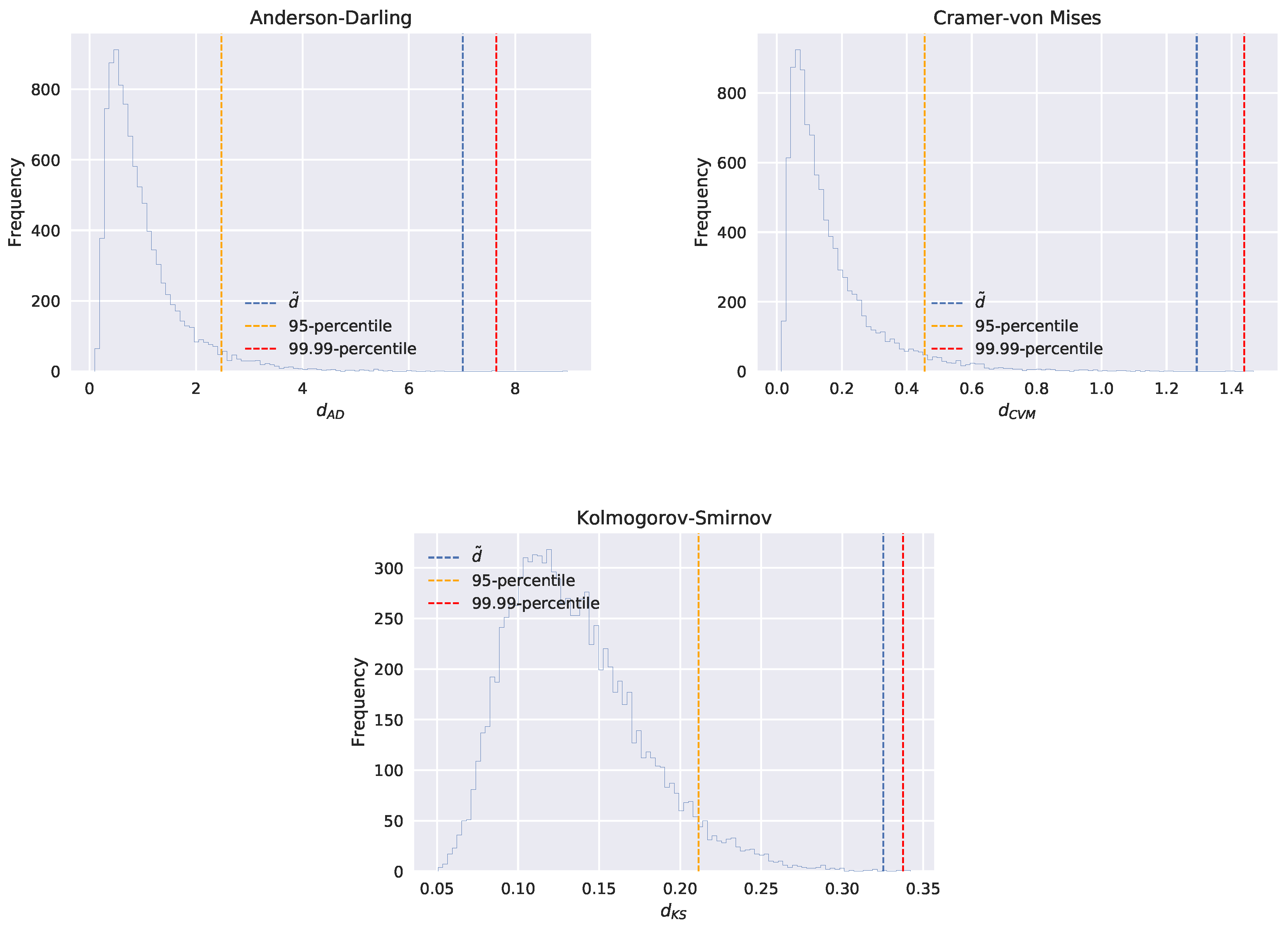
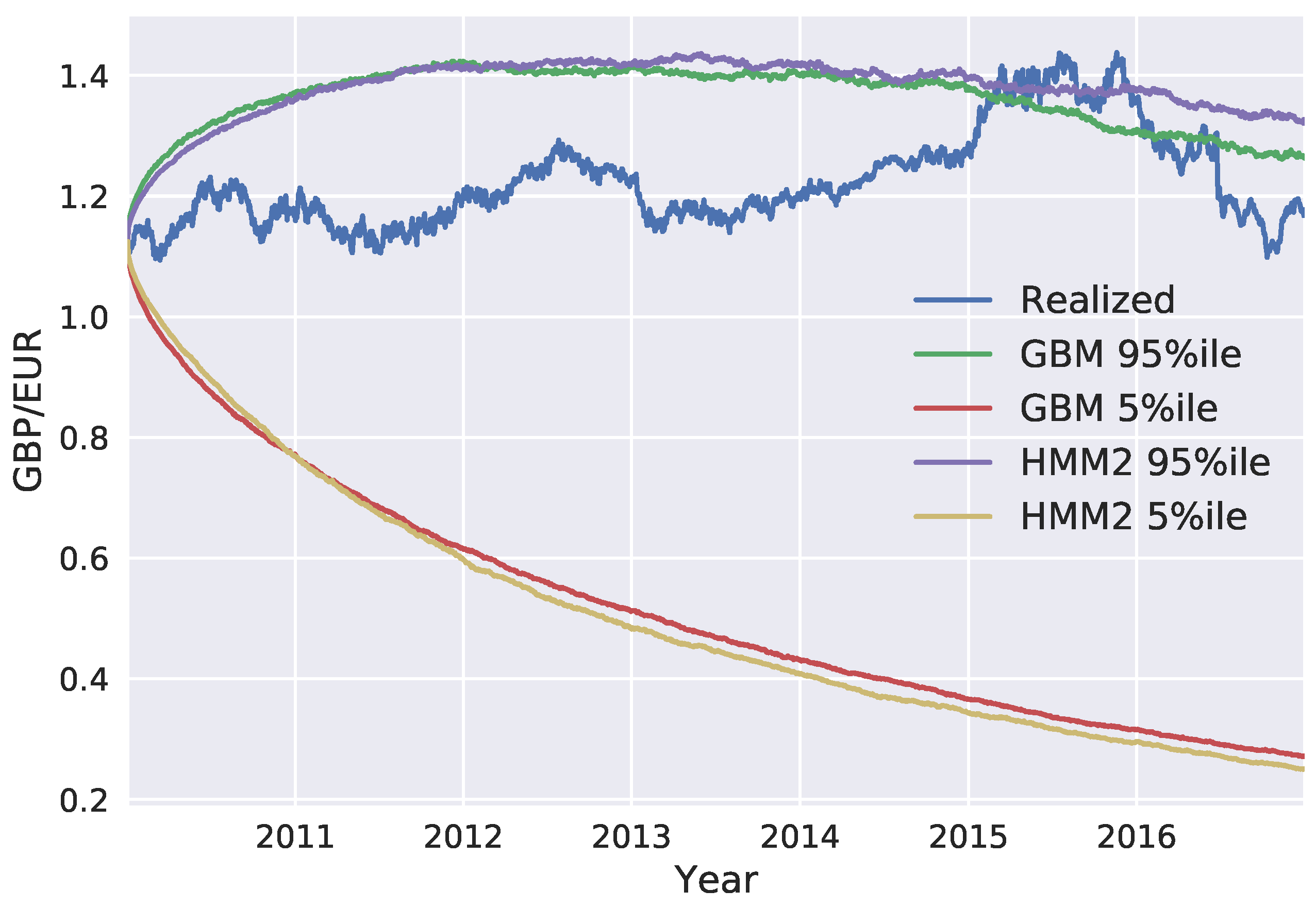
We generated exchange rate scenarios for four currency pairs: USD/EUR, GBP/EUR, RUB/EUR, and MXN/EUR. A risk factor evolution model backtesting exercise was performed, in line with Basel III requirements, and the the percentiles of the long-term distribution cones were obtained. The performances of the one-state and two-state models (GBM and the two-state HMM, respectively) were found to be very similar, with the two-state model HMM being slightly more conservative. However, when the generated scenarios were used to calculate exposure profiles for options on the RUB/EUR exchange rate, we found significant differences between the results of the two models. These differences were even more pronounced for deep out-of-the-money options.

Our study highlights some of the limitations of backtesting as a tool for comparing the performance of RFE models. Backtesting can be a useful way to objectively assess model performance. However, it can only be performed over short time horizons; with our available data, we could perform a statistically sound test of modeling assumptions for a time horizon of maximum length three months. It is, therefore, important to put effort into the interpretation of backtesting results, before they are translated into conclusions about model performance. Our results show how two models with similar performances in a backtesting exercise can result in very different exposure values and, consequently, in very different regulatory and economic capital buffers. This can lead to regulatory arbitrage and potentially weaken financial stability and, further, turn into a systemic risk.

The research presented in this paper can be extended in a number of ways, such as considering the evolution of risk factors other than exchange rates. Another topic worthy of investigation is the enhancement of the backtesting framework presented by Ruiz (2014), by considering statistical tests similar to the ones presented by Berkowitz (2001) and Amisano and Giacomini (2007). Finally, an interesting research direction is the development of an agent-based simulation model with heterogeneous modeling approaches, with regards to the RFE models. This model could potentially give valuable insights into the impact of heterogeneous models in financial stability.

References

1. Amisano, Gianni, and Raffaella Giacomini. 2007. Comparing density forecasts via weighted likelihood ratio tests. Journal of Business & Economic Statistics 25: 177–90. [Google Scholar]
2. Anfuso, Fabrizio, Dimitrios Karyampas, and Andreas Nawroth. 2014. Credit exposure models backtesting for Basel III. Risk. September. Available online: https://www.risk.net/2362332 (accessed on 1 March 2019).
3. Ang, Andrew, and Geert Bekaert. 2004. How regimes affect asset allocation. Financial Analysts Journal 60: 86–99. [Google Scholar] [CrossRef]
4. Basel Committee on Banking Supervision. 1996. Supervisory Framework for the Use of “Backtesting” in Conjunction with the iNternal Models Approach to Market Risk Capital Requirements. Basel: Basel Committee on Banking Supervision. [Google Scholar]
5. Basel Committee on Banking Supervision. 2010a. Basel III: A Global Regulatory Framework for More Resilient Banks and Banking Systems. Basel: Bank for International Settlements. [Google Scholar]
6. Basel Committee on Banking Supervision. 2010b. Sound Practices for Backtesting Counterparty Credit Risk Models. Basel: Bank for International Settlements. [Google Scholar]
7. Basel Committee on Banking Supervision. 2014. The Standardised Approach for Measuring Counterparty Credit Risk Exposures. Basel: Bank for International Settlements. [Google Scholar]
8. Baum, Leonard E., and John Alonzo Eagon. 1967. An inequality with applications to statistical estimation for probabilistic functions of Markov processes and to a model for ecology. Bulletin of the American Mathematical Society 73: 360–63. [Google Scholar] [CrossRef]
9. Baum, Leonard E., and Ted Petrie. 1966. Statistical inference for probabilistic functions of finite state Markov chains. The Annals of Mathematical Statistics 37: 1554–63. [Google Scholar] [CrossRef]
10. Berkowitz, Jeremy. 2001. Testing density forecasts, with applications to risk management. Journal of Business & Economic Statistics 19: 465–74. [Google Scholar]
11. Bollen, Nicolas P. B. 1998. Valuing options in regime-switching models. The Journal of Derivatives 6: 38–49. [Google Scholar] [CrossRef]
12. Boothe, Paul, and Debra Glassman. 1987. The statistical distribution of exchange rates: Empirical evidence and economic implications. Journal of International Economics 22: 297–319. [Google Scholar] [CrossRef]
13. Bulla, Jan, Sascha Mergner, Ingo Bulla, André Sesboüé, and Christophe Chesneau. 2011. Markov-switching asset allocation: Do profitable strategies exist? Journal of Asset Management 12: 310–21. [Google Scholar] [CrossRef]
14. Dempster, Arthur P., Nan M. Laird, and Donald B. Rubin. 1977. Maximum likelihood from incomplete data via the em algorithm. Journal of the Royal Statistical Society. Series B (Methodological) 39: 1–38. [Google Scholar] [CrossRef]
15. Diebold, Francis X., Todd A. Gunther, and Anthony Tay. 1997. Evaluating density forecasts. International Economic Review 39: 863–83. [Google Scholar] [CrossRef]
16. Garman, Mark B., and Steven W. Kohlhagen. 1983. Foreign currency option values. Journal of international Money and Finance 2: 231–37. [Google Scholar] [CrossRef]
17. Ghahramani, Zoubin. 2001. An introduction to hidden Markov models and bayesian networks. In Hidden Markov Models: Applications in Computer Vision. Singapore: World Scientific, pp. 9–41. [Google Scholar]
18. Gregory, Jon. 2012. Counterparty Credit Risk and Credit Value Adjustment: A Continuing Challenge for Global Financial Markets. Hoboken: John Wiley & Sons. [Google Scholar]
19. Guidolin, Massimo, and Allan Timmermann. 2007. Asset allocation under multivariate regime switching. Journal of Economic Dynamics and Control 31: 3503–44. [Google Scholar] [CrossRef]
20. Guo, Xin. 2001. An explicit solution to an optimal stopping problem with regime switching. Journal of Applied Probability 38: 464–81. [Google Scholar] [CrossRef]
21. Hamilton, James D. 1988. Rational-expectations econometric analysis of changes in regime: An investigation of the term structure of interest rates. Journal of Economic Dynamics and Control 12: 385–423. [Google Scholar] [CrossRef]
22. Hamilton, James D. 1989. A new approach to the economic analysis of nonstationary time series and the business cycle. Econometrica: Journal of the Econometric Society 57: 357–84. [Google Scholar] [CrossRef]
23. Hull, John C. 2009. Options, Futures, and Other Derivatives, 7th ed. New York: Pearson Prentice Hall. [Google Scholar]
24. Juang, Biing Hwang, and Laurence R. Rabiner. 1991. Hidden Markov models for speech recognition. Technometrics 33: 251–72. [Google Scholar] [CrossRef]
25. Krogh, Anders, Michael Brown, I. Saira Mian, Kimmen Sjölander, and David Haussler. 1994. Hidden Markov models in computational biology: Applications to protein modeling. Journal of Molecular Biology 235: 1501–31. [Google Scholar] [CrossRef]
26. Naik, Vasanttilak. 1993. Option valuation and hedging strategies with jumps in the volatility of asset returns. The Journal of Finance 48: 1969–84. [Google Scholar] [CrossRef]
27. Nystrup, Peter, Bo William Hansen, Henrik Madsen, and Erik Lindström. 2015. Regime-based versus static asset allocation: Letting the data speak. The Journal of Portfolio Management 42: 103–9. [Google Scholar] [CrossRef]
28. Nystrup, Peter, Henrik Madsen, and Erik Lindström. 2015. Stylised facts of financial time series and hidden Markov models in continuous time. Quantitative Finance 15: 1531–41. [Google Scholar] [CrossRef]
29. Picoult, Evan. 2002. Quantifying the Risks of Trading. Cambridge: Cambridge University Press. [Google Scholar]
30. Rabiner, Lawrence R. 1990. A tutorial on hidden Markov models and selected applications in speech recognition. In Readings in Speech Recognition. Amsterdam: Elsevier, pp. 267–96. [Google Scholar]
31. Ruiz, Ignacio. 2014. Backtesting counterparty risk: How good is your model? The Journal of Credit Risk 10: 87. [Google Scholar] [CrossRef]
32. Rydén, Tobias, Timo Teräsvirta, and Stefan Åsbrink. 1998. Stylized facts of daily return series and the hidden Markov model. Journal of Applied Econometrics 13: 217–44. [Google Scholar] [CrossRef]
33. Wilson, Andrew D., and Aaron F. Bobick. 1999. Parametric hidden Markov models for gesture recognition. IEEE Transactions on Pattern Analysis and Machine Intelligence 21: 884–900. [Google Scholar] [CrossRef]
34. Zhu, Steven H., and Michael Pykhtin. 2007. A guide to modeling counterparty credit risk. GARP Risk Review 37. July/August. Available online: https://ssrn.com/abstract=1032522 (accessed on 11 June 2019).
35. Zucchini, Walter, Iain L. MacDonald, and Roland Langrock. 2016. Hidden Markov Models for Time Series: An Introduction Using R. London: Chapman and Hall/CRC. [Google Scholar]
Figure 1. A hidden Markov model (HMM) with two states and three discrete observations, where a i j is the probability of transition from state X i to state X j and b j ( k ) is the emission probability for symbol v k in state X j .
Risks 07 00066 g001
Figure 2. Examples of the three-color scoring scheme. The model in the example receives yellow scores for all three metrics, as d y < d ˜ < d r .
Risks 07 00066 g002
Figure 3. Akaike information criterion (AIC) and Bayesian information criterion (BIC) for HMMs calibrated using USD/EUR time-series.
Risks 07 00066 g003
Figure 4. AIC and BIC for HMMs calibrated using GBP/EUR time-series.
Risks 07 00066 g004
Figure 5. AIC and BIC for HMMs calibrated using RUB/EUR time-series.
Risks 07 00066 g005
Figure 6. AIC and BIC for HMMs calibrated using MXN/EUR time-series.
Risks 07 00066 g006
Figure 7. Percentiles of long-term distribution cones for USD/EUR under GBM and HMM with two states.
Risks 07 00066 g007
Figure 8. Percentiles of long-term distribution cones for GBP/EUR under GBM and HMM with two states.
Risks 07 00066 g008
Figure 9. Percentiles of long-term distribution cones for RUB/EUR under GBM and HMM with two states.
Risks 07 00066 g009
Figure 10. Percentiles of long-term distribution cones for MXN/EUR under GBM and HMM with two states.
Risks 07 00066 g010
Figure 11. Credit exposure values for out-of-the-money (OTM) call options on the RUB/EUR exchange rate (a) and the impact of using a two-state HMM, instead of a GBM (b).
Risks 07 00066 g011