Abstract
This paper captures and measures the longevity risk generated by an annuity product. The longevity risk is materialized by the uncertain level of the future liability compared to the initially foretasted or expected value. Herein we compute the solvency capital (SC) of an insurer selling such a product within a single risk setting for three different life annuity products. Within the Solvency II framework, we capture the mortality of policyholders by the mean of the Hull–White model. Using the numerical analysis, we identify the product that requires the most SC from an insurer and the most profitable product for a shareholder. For policyholders we identify the cheapest product by computing the premiums and the most profitable product by computing the benefit levels. We further study how sensitive the SC is with respect to some significant parameters.
1. Introduction
During the past decade, pension funds and insurers have faced numerous problems as consequences of the continuous increase of population life expectancy commonly called longevity risk. Due to the longevity risk, insurers were obliged to increase the annuity prices in order to be more confident with regard to their solvency towards the policyholders. In order to protect the policyholders against such fluctuations of insurance product prices, the legislator has settled some regulatory rules called the Solvency II (SII) (see European Insurance and Occupational Pensions Authorit (2014a); European Insurance and Occupational Pensions Authorit (2014b)). The particularities of the SII framework are based on its risk-sensitivity and its multi-risk factors; the latter means it recognizes that insurers face different kinds of risks, such as the equity, the longevity and the interest rate risks. In this regard, insurers have to focus on the computation of the so called solvency capital (SC) as defined in the SII regulation. By solvency capital, we refer to the amount the insurance company or the insurer has to put aside in order to be solvent until the end of the contract in accordance with the SII regulation. In the literature, a few authors proposed substantiated mathematical definitions of the solvency capital requirement (SCR). Liebwein (2006) gave an overview of internal risk models in the context of SII and some of their applications beyond SII. Kochanski and Karnarski (2011) proposed in 2011 a partial internal model to determine the solvency capital requirement for static and dynamic hybrid products. Some researcher gave a mathematical definition of the SCR computed at contract inception (see Barrieu et al. (2012) and Devineau and Loisel (2009)), whereas Ohlsson and Lauzeningks (2009) gave a definition of the SCR at any time during the contract lifetime. In 2012, (Christiansen and Niemeyer (2014)) presented some similarities and differences of the various interpretations and definitions of the SCR. Pfeifer and Strassburger (2008) showed that some SCR methods proposed and discussed in the literature have stability problems.
As a consequence of the SII regulation, insurers have to be aware of the level of their SC at any time t from the contract inception until the end of the contract. As capital, the SC can be invested in a risky asset with limited liability, such as a stock, or in a risk-free asset, such as bonds. In this article, we focus on the longevity risk; thus, we assume the SC to be invested in a risk-free asset.
The longevity risk is nowadays a major issue for pension funds and insurance companies. For pension funds and insurance companies, this is materialized by the uncertain level of the future liability compared to the expected value. Many authors have proposed models to assess and to hedge the longevity risk and its effect on pension funds or life insurance. Antolin (2007) examined in 2007 how longevity risk affects employer-provided pension plans. Researchers have developed longevity risk hedging instruments, such as the longevity swap proposed by Blake and Burrows (2001). Fung et al. (2019) proposed a tractable stochastic mortality model with age dependent drift and volatility. They derived analytical formulae for prices of longevity derivatives. In this paper we focus on annuities (see Brown et al. (2000)). Hari et al. (2008) analyzed the importance of longevity risk for the solvency of portfolios of pension annuities; they distinguished two types of mortality risk: the micro-longevity risk, which quantifies the risk related to uncertainty of the time of death, and the macrolongevity risk, which is due to uncertain future survival probabilities. We consider the second type of mortality, i.e., the macrolongevity risk, and we consider three annuity products: the lifetime, the deferred and the term annuities. These will be used in order to measure the longevity risk borne by an insurer selling such annuities, and our measurement approach consists of assessing the SC of the insurer. Moreover, the mortality of the policyholder is captured by a mortality model. Many researchers have developed a large range of mortality models—the Vasicek model, Hull–White model, Gompertz model, etc. We capture the mortality of the policyholder by the Hull–White model for which we assume a Gompertz model mean reversion level.
Several authors and insurance companies focus on the issue of SC assessment for life annuity products. Olivieri and Pitacco (2008) investigated rules for evaluating the SC by a portfolio of life annuity to meet longevity risk. This problem has also been solved for the case of multiple premiums and single cash flow as well as for the case of single premium and single cash flow within a Brownian motion driven market by Devolder and Lebègue (2017). Therefore, our goal here is on one hand, to extend the results presented in the latter article within an longevity risk market, i.e., to compute the SC in the case of multiple cash flows with single premium; and on the other hand, to compare the three annuities using the results for both the insurer and the policyholders. By longevity risk market, we refer to a market fully hedged against any other risks differently from the longevity risk; this is called the longevity model. A common difficulty usually encountered both in practice or in research while dealing with such a problem is the numerical results; i.e., the simulation methods. Several authors have proposed efficient and robust simulation methods. Bauer et al. (2010) proposed a mathematical framework for the computation of the SC using the least square Monte Carlo method. Baue et al. (2012) provided a framework to compute the SC using nested Monte carlo simulations. Hainaut et al. (2007) proposed a robust framework to approximate the SCR by the value-at-risk (VaR) for a life insurance policy with death benefits. Regarding the simulation method used in this work, we used the nested Monte carlo simulations. Moreover in order to be consistent with SII framework, we used the VaR as the risk measurement and considered both a constant and a variable confidence level.
Our contribution comes from the deep comparative analysis of the three annuities with respect to the longevity risk generated by each, first from the policyholders point of view, and secondly from the insurer’s viewpoint. From the policyholders viewpoint, we compare both the values of benefit payouts and the single premium, whereas from the insurer’s viewpoint we compare the SC obtained for each product. Furthermore, we show by computing the internal rate of return that adding a SC could be seen as an investment for shareholders, and we compare the three annuities through their internal rates of return. This latter comparison is made based on the mean-variance approach; in other words, we compare both the mean and the variance of the internal rate of return of each product. We found that the deferred annuity requires the most SC and the most profitable product for a constant confidence level, whereas for variable confidence levels we found that the term annuity requires the most SC and the least profitable product.
The remaining part of this paper is structured as follows. In the next section, we present features of our model in detail; for instance, we present the mortality model and the insurer liability. The theoretical results are presented in Section 3 where we develop the formulas of the SC for a deferred annuity. Section 4 presents the numerical results and the comparative remarks drawn from numerical results. These comparisons are made from the insurer, shareholder and policyholder viewpoints, with respect to the annuities, the confidence levels and the values of the interest rate. Finally, Section 5 concludes.
2. The Model’s Features
In this section, we focus on the general framework for our model. Before discussing the used products and the mortality model, we provide an overview of the financial market and the assumptions needed subsequently. In this work, we assume that the insurance company is fully hedged against any other risks except the longevity risk: the implied model is called the longevity model. We assume that the only asset available in the market is a risk-free asset: a discount bond ; that is, the value at time t of a financial instrument that pays a unit of currency at maturity time n. Therefore, in order to focus (or measure) only the longevity risk, we consider the discount bond to be defined using a deterministic, short rate process ; i.e., (see Vasicek and Fong (2015)).
2.1. Mortality Model
This subsection presents in detail the mortality model used to capture the policyholders’ real survival probabilities. We develop the theory behind the chosen model; this allows us to explicitly express both the liability of the insurer and the annual benefit received by the policyholders.
As extension of the approach presented in Devolder and Lebègue (2017) (where the force of mortality is modelled using the Ornstein–Uhlenbeck process), and following Zeddouk and Devolder (2019), we model the force of mortality of the cohort by the Hull–White process. Note that our approach can be extended to other continuous mortality models. The dynamic of the force of mortality is then defined by Lichters et al. (2015)
where is the mean reversion rate; is the absolute volatility of ; is a Brownian motion; is the affiliation age; and represents the mean reversion level function. We suppose that is given by the Gompertz mortality model Gompertz (1825)
where is the baseline mortality and is the senescent component. Using an arbitrary starting time , from short calculations we get
this represents in fact the force of mortality at time s of an individual initially of age and alive at time t (i.e., age ). Let us now consider the survival index at time s of an individual initially of age , alive at time t and surviving more years defined by the random variable
with Z being a normally distributed random variable with mean zero and variance one denoted by . One now can show that
where
and
We will measure only the longevity risk borne by the insurer; to that end we consider a cohort of retirees; i.e., . Hence, the number of survivors at any time is given by
Note that n is the duration of the contract. Let us denote by the (physical) probability for a policyholder of age 65 and alive at age , to survive until age for
where is the sigma algebra at time t, it encodes the information available at t.
and
is a measurable at time t. Moreover, we assume that represents the mortality table guaranteed by the insurer at the contract inception; that is the best estimate of the survival index (from ); note that .
From this, we can then value the liability of the insurer at any time of the contract. Note that if is the duration of the contract, then a -year deferred annuity can be seen as a generalization of both the lifetime and the term annuity. Indeed, setting , we obtained a lifetime annuity and for a fixed , substituting n by and setting we obtained a term annuity. Hence, we develop in this paper a detailed analysis for d-year deferred annuity for which we can deduce the cases of both lifetime and term annuity using the given transformations.
2.2. Insurer’s Liability
The contract consists of an initial cohort of individuals paying each an amount to an insurer at inception in order to receive an annual amount of R during a period depending of the annuity purchased. We then denote the cohort’s single premium by and the cohort (random) annual benefit by ; note that the cohort initial benefit is denoted by .
It is important to stress that throughout this article in order to design the mortality model, we consider an initial cohort of retirees at inception for which we model the longevity risk by a stochastic mortality model (the HW model). In other words, we measure the longevity risk only on the decumulation period (i.e., the period after the retirement) and we do not consider the accumulation period (i.e., period before retirement). The parameters of the HW mortality model are supposed to be known from inception and they are valid only for the initial cohort from which they have been computed. This statement is equivalent to the hypothesis of no model and parameter risks considered all along this article.
The value of the cohort’s annual benefit for a d-year deferred annuity is defined based on an initially guaranteed life table assumed to describe the cohort’s mortality on the decumulation period. Moreover, we assume the value of the cohort’s premium invested on the discount bond until time to be equal to the value at time of the discounted annual benefits. The insurer total liability at time d with respect to the initially guaranteed life table for a deferred annuity is given by the expected value of the liability of the insurer. That is
represents in fact the value at time d of the overall benefits invested in a discount bond that the insurer has to pay to the policyholders alive at each payment time according to the initially guaranteed survival probability in the case of a lifetime annuity, and n is the duration of the contract. Therefore, we assume the single premium to be defined as , where is given by Formula (5); this implies that , and hence the individual annual benefit is given by
The formula of the annual benefit of a -year-term annuity is obtained just by substituting n by and setting ; for a lifetime annuity we only set . Next we compute the SC at any time of the contract for the three annuities (lifetime, deferred and term annuities) in order to compare the obtained numerical results. To this end, we develop the formulae of the SC in the next section for d-year deferred annuity. As mentioned previously, we consider a cohort of retirees initially of age .
3. Solvency Capital Valuation
In this section, we present the formulae of the SC for a d-year deferred annuity form which we can deduce the formulae of a -year term and lifetime annuities. As reminder, both the initial premium and the SC are invested in a discount bond. In order to measure the SC, we adopt in this paper a more general view than the standard approach proposed by the SII. Taking into account the very long term horizon of this kind of product, we use a maturity approach and not a one year measure, as stated by the SII. We value the SC by the use of a risk measure applied to the final surplus so as to measure the global longevity risk borne by the insurer. This method has been used for other products, as proposed by Devolder and Lebègue (2017). More precisely, in order to take into account the multi period character of the product, we consider the static risk measure VaR as our risk measurement tool with an annual confidence level of as stated by SII (see European Insurance and Occupational Pensions Authorit (2014a), European Insurance and Occupational Pensions Authorit (2014b)). Then, we assume the temporal independence of events and we consider constant and equal yearly confidence level such that for a n-maturity contract, the overall confidence level is . We further consider also a fixed constant confidence level of . These two values of the confidence level are used for simulation purposes in order to highlight the impact of the confidence level considered on the level of SC.
We consider a policyholder buying a -year deferred annuity at inception time . We will value the SC of the insurer within the computational intervals defined above. It is important to stress that the payment stream of a given policyholder begins if and only if he or she is alive at time ; i.e., at age . Additionally, the individual annual benefit for a d-year deferred annuity is given by Formula (6). Note that we have two computational intervals: the deferred period and the payment period .
3.1. Deferred Period
Our approach of assessing the SC consists of measuring the risk of having a negative final surplus at time . By final surplus, we refer to the amount of assets that exceeds the liability of the insurer at the end of the contract. Mathematically, let
- -
- be the fund value at the end of the contract, where the available asset at time t is defined as
- -
- be the value at time n of the liability of the insurer;
- -
- is then the final surplus of the contract.
Therefore, it follows from our maturity approach for the valuation of the SC that at the computational time t, the SC satisfies the following condition.
One can show that in this period, for any the definition of the SC given by Formula (8) is equivalent to
where is given by (7) and the value at term of the liability are given by
where for any
- -
- is the real number of survivors at time t;
- -
- is the survival index of an annuitant initially aged 65, alive at age and living at least up to age . This term guarantees that a policyholder in the cohort must be alive at the end of the deferred period;
- -
- guarantees that benefits are paid if the annuitant is alive at each payment time on the payment period.
3.2. Payment Period
On this other interval the SC is valued with respect to the remaining liabilities at term which are the unpaid benefits yearly deduced from the asset and evaluated at term. Moreover, we have to take into account the already paid benefits; i.e., the benefits paid up to time t. This is achieved using the fact that information up to time t is known, meaning that the number of survivors at t is known. Hence, the SC satisfies the following
where represents the total unpaid benefits at n and it is given by
Note that for , is known as the realized number of survivors; moreover, the asset is given by
The second term of the right hand side represents the value at t of the benefits paid up to time t.
Note that concerning a -year-term annuity, the payment stream begins at inception, i.e., age , and ends after years, with . Therefore, the formulae of a -year-term annuity can be obtained from the previous formulae by setting and . For a lifetime annuity, we only set in the previous formulae, and for both a term and a lifetime annuities, we have only one computational period: the decumulation period, which is equal to the payment period.
4. Numerical Results
Some graphical representations and some numerical values of the SC with respect to the computational time t, the length of the deferred period d and the term in the case of lifetime, deferred and term annuities, are presented in this section.
4.1. Simulation Framework
The simulation of the longevity SC is made in two steps: we first calibrate the HW model (see Lichters et al. (2015)), and secondly, we make use of the Monte Carlo (MC) simulations of the VaR (see Glasserman (2013)). For the calibration of the Hull–White model (1), we need some real data and a calibration method. To do so, we consider the unisex projected generational life table of an individual aged 65 in 2015 for an ultimate age of 110 in 2060 available on the IA|BE life table published in 2015 Antonio et al. (2015). Using this data, we calibrate the HW model (1) by the use of the mean squared error (MSE); and we obtain the following parameters in Table 1.

Table 1.
Calibration parameters of the HW model using MSE.
The obtained calibration parameters of the force of mortality fit the IA|BE data well, since the MSE .
As for the MC simulations, we use the nested MC simulations Baue et al. (2012). We consider a cohort of size all aged 65 at the affiliation date . Each participant pays to the insurer at in order to receive a constant amount R depending on the annuity bought. We further consider the following parameters
where n represents the duration of the contract, and assuming means we consider an ultimate age of 110. As for the term annuity, we suppose ; this means the contract will end when the policyholder is aged 80 with a maximum of 16 possible benefits. For the deferred annuity, we take ; i.e., the payments start when the annuitants are aged and ends when they are aged 110.
Moreover, as the force of mortality at a time t depends on the force of mortality at time , we consider for simulation purposes the correlation between two consecutive survival indexes and ; this implies that the liability at time n for a d-year deferred annuity computed at inception takes the form
where by the use of Cholesky decomposition Ng and Li (2011), we have
where the s are normally distributed random variables with mean zero and variance one. Note that is independent of ; and where is given by Formula (3).
4.2. Results and Comparative Remarks
In order to guide their decision making, we provide the insurer as well as the shareholders with information about the impact of the longevity risk on each of the three annuities. Moreover, for annuitants, we provide a comparative study on both the benefits and the initial premium for the three annuities with respect to some parameters. This could help annuitant in deciding which product to buy, depending on their risk aversion. This comparison is made based on both the level of the annual benefit (for a fixed single premium) and the level of the single premium (for constant annual benefits), which are different from one annuity to another. From the insurer’s viewpoint, the comparison is made using the level of the SC of each different annuity and the internal rate of return on the SC invested by shareholders.
Regarding the policyholders on the one hand, considering a fixed single premium for each of the annuities, we obtained from some computations that the amount of annual benefit differs from one annuity to another annuity following the relations
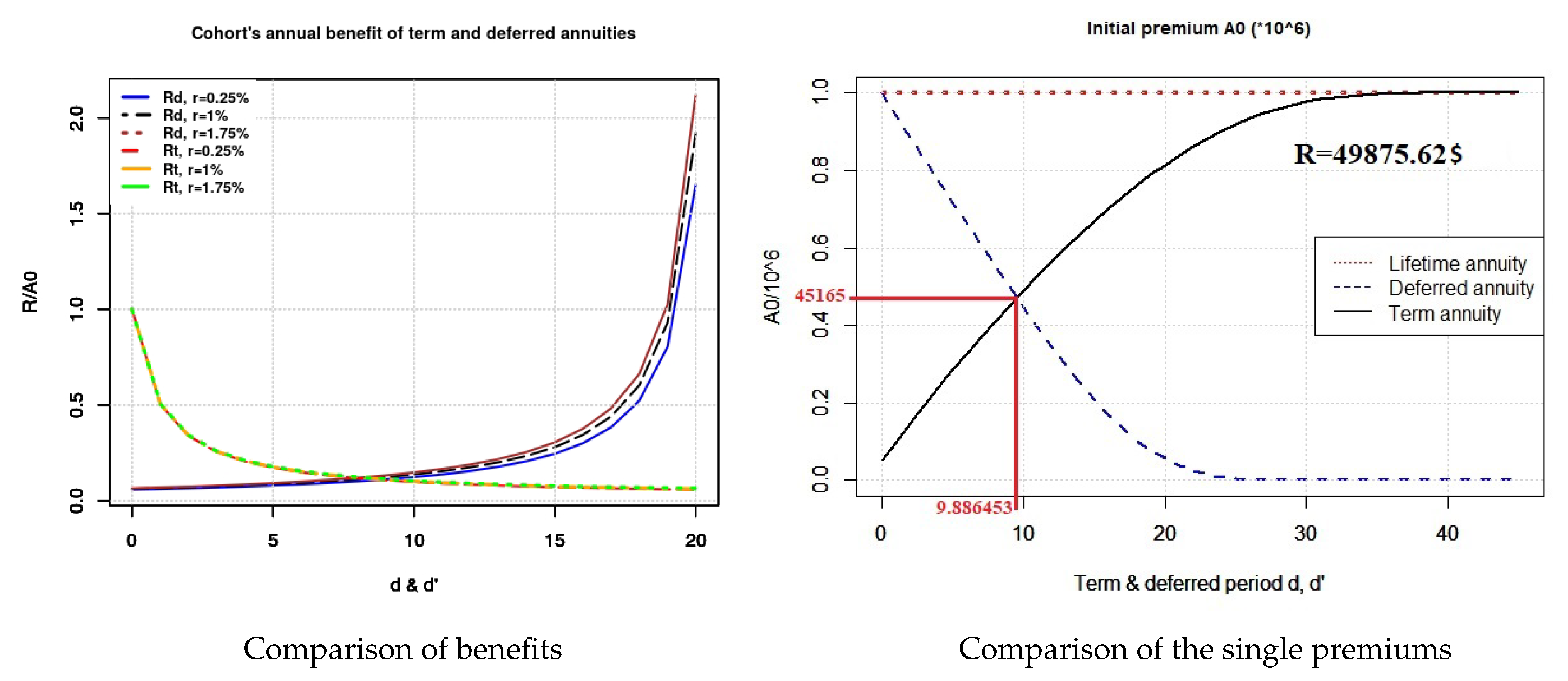
In fact, this can be seen in Figure 1 and can be justified as follows.
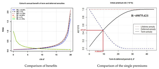
Figure 1.
Annual benefits for equal premiums and premiums for equal annual benefits.
- : This comes from the fact that , where is shared for the benefits for the lifetime annuity, whereas is shared for the benefits for term annuity. This can be explained by the fact that the survival probabilities are high for the first years following the retirement.
- : Similarly, the unique premium is distributed into benefits for a lifetime annuity, whereas it is distributed into benefits for the deferred annuity.
Moreover, one can show that if and only if
This is shown in Figure 1 where we observe that there exit some values of d and such that the benefits of deferred and term annuities are equal. Note that the comparison of and depends on the values of d and respectively. In fact increases with d, whereas decreases when increases.
On the other hand, we consider constant annual benefits for each of the annuities assumed to be
where and . The comparison will follow from Figure 1 which represents both the annual benefit per unit of initial premium with respect to d and , and the variation of the single premium of a term annuity () and the deferred annuity () for fixed benefit with respect to d and .
We observe on the right graph of Figure 1 that and have opposite behaviors; in fact converges to , whereas converges to 0, and they coincide at . In particular, for and we have and ; it follows that for equal level of annual benefits, a 16-year deferred annuity is cheaper than a 15-year immediate-term annuity, which in turn is cheaper that an immediate lifetime annuity.
Concerning the insurer’s viewpoint, the behavior of the SC is presented in the following graphs
- •
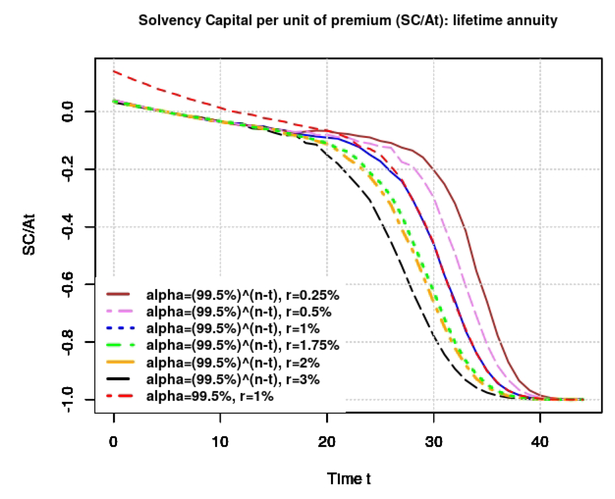
- Lifetime annuity:Figure 2 shows how the SC changes with respect to the computational time for different values of the confidence level and the short rate. We observe that the SC decreases when the short rate increases. We can also see that the SC decreases as t increases. Moreover the values of SC obtained with a variable confidence level are smaller than those obtained with a constant confidence level.
 Figure 2. Lifetime annuity; for different values of the short rate r and .Note that a negative value of SC means no additional capital is required from the insurer; that is, . In other words, means that the insurer is solvent with a confidence level without any additional capital.
 - •
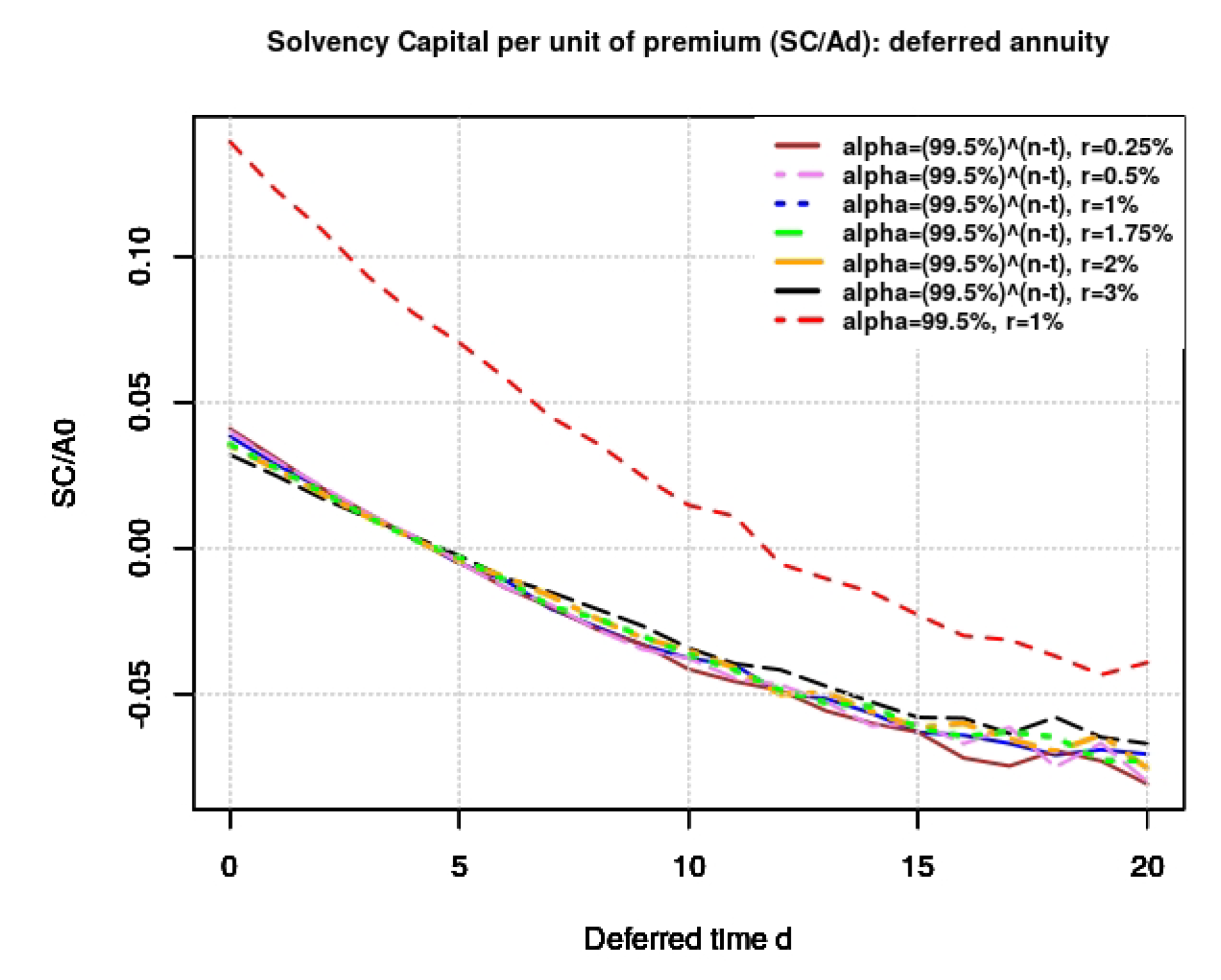
- Deferred annuity: Below are presented the graphs of the SC with respect to t; to d on the deferred period in Figure 3, and with respect to d on the payment period in Figure 4 respectively.
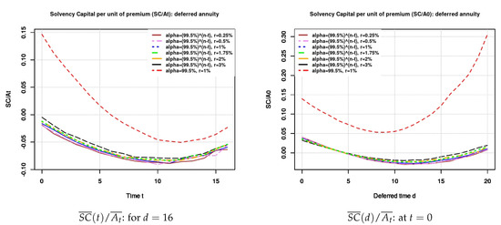 Figure 3. Deferred annuity; and respectively for different values of the short rate r and on the deferred period.
 Figure 4. Deferred annuity; at for different values of the short rate r and on the payment period.From Figure 3 it comes out that the SC decreases for both values of and slightly decreases with respect to r. Furthermore, for a constant confidence level we obtain a higher value of SC; it decreases for small values of d and increases for larger values of t. Moreover, the SC have a convex form with respect to d and with respect to t. This implies that there exist optimal values of d and t that minimize the SC of the insurer.Regarding Figure 4, it can be seen how the SC decreases with d in the payment period. Moreover, we find that the SC is strictly negative with respect to and for any value of r and .
 - •
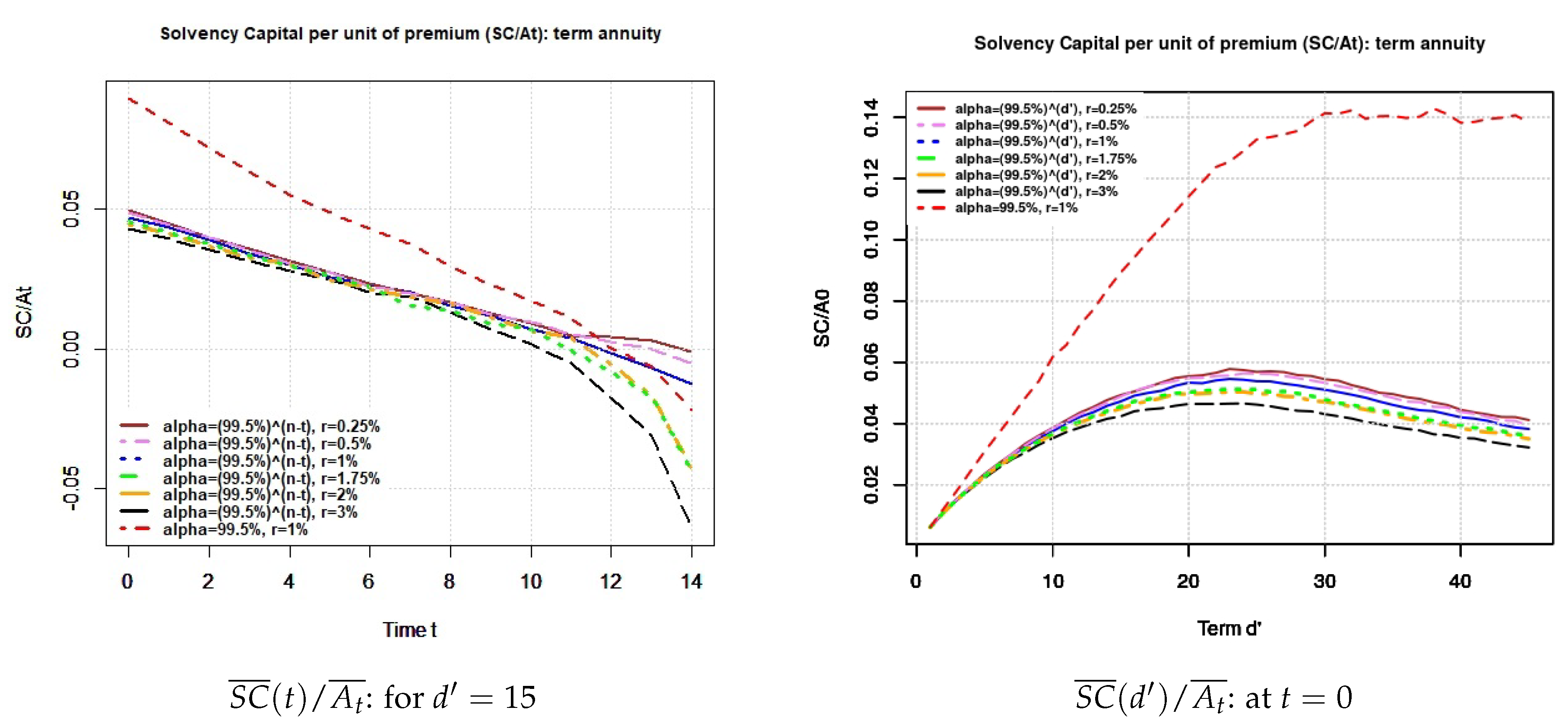
- Term annuity:Figure 5 below shows the SC with respect to t and to both .
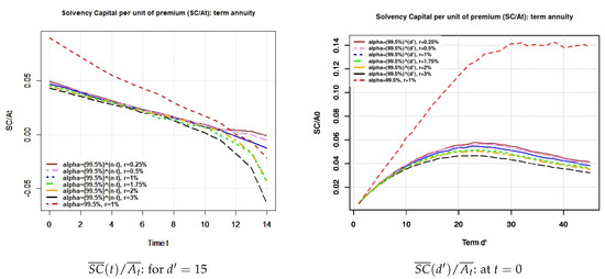 Figure 5. Term annuity; and respectively for different values of the short rate r and .It comes out that the SC decreases with and r. Moreover, the SC is strictly positive and increases with for constant and takes a concave form when increases for variable values of .
From these figures, one could infer that the product requiring the lower amount of SC does depend on the time at which the said SC is computed. For example, for variable and , worth zero for the lifetime annuity, it is worth for the term annuity and it is zero for the deferred annuity. Hence, one might say that the term annuity requires the most SC at that computational time. Thus it will be harsh to point a particular product to be the best for an insurer, as the comparison has to be made at same points in time. Table 2 below shows the values of the SC at inception (i.e., at ) for and .

Table 2.
Comparison of the annuities at .
It follows that the constant confidence level gives higher SC compared to the variable confidence level. This can be explained by the fact that the required probability of default with a constant is larger than that of the variable . Moreover Table 2 also shows that for variable , the deferred annuity requires the lesser SC followed by the lifetime annuity. For constant , the deferred annuity requires the most SC followed by the lifetime annuity. Note that the negative SC obtained for the deferred annuity means that the insurer has no additional capital to put aside in order to guarantee his solvency; i.e., . Values of for immediate annuity are present in Table A1 in Appendix A.
Note that an alternative way to compare these products could be from the shareholder point of view: one could assess the ability of a given annuity to generate benefit from the SC invested on it. This ability can be assessed by the internal rate of return (IRR) on the SC Gronch (1986). Hence, having this rate be greater than the short rate indicates an advantageous investment for shareholders, whereas a IRR less than the short rate implies an investment with loss compared to the risk-free investment. Moreover, for IRR , the shareholder will just take back the initial capital invested at , and the worst case (i.e., loosing the whole initial capital) would be when IRR . By definition, the SC satisfies
The possible benefit at the end of the contract called the final surplus is a random variable given by
It follows that the IRR, denoted by is a random variable satisfying the following
thus, the IRR on the SC is given by
where
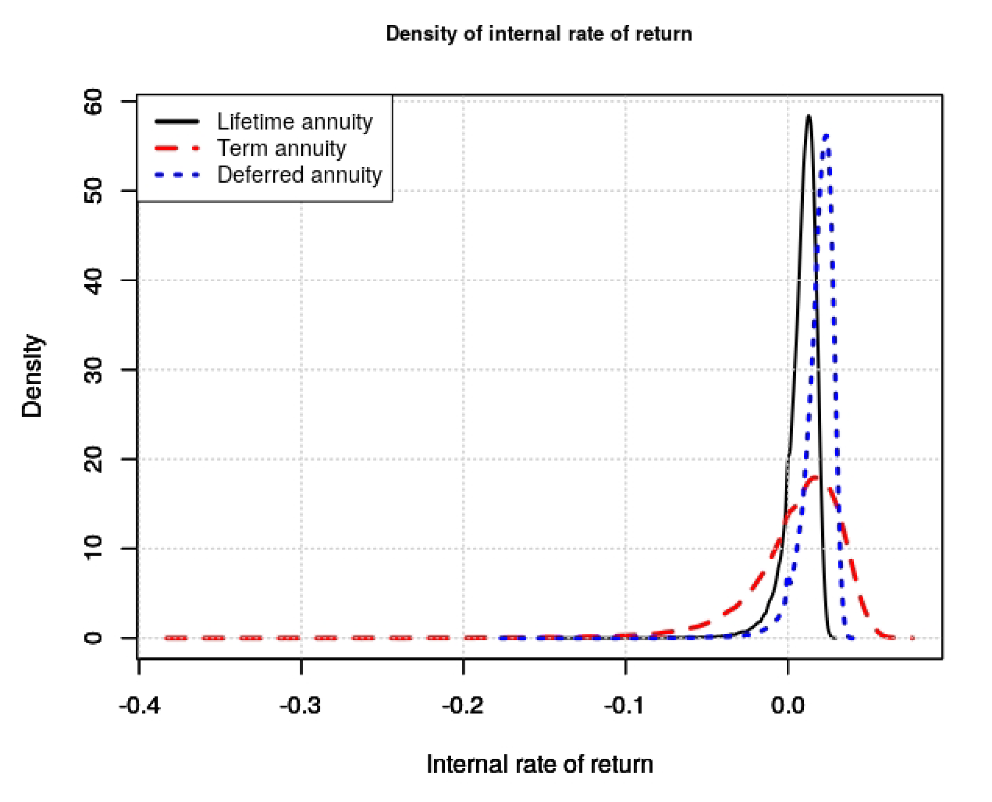
It is important to stress that the IRR is computed if and only if the SC is strictly positive. For comparison purpose, Figure 6 and Table 3 respectively show the density and the numerical values of mean and variance of the IRR for the three annuities computed at , for and .
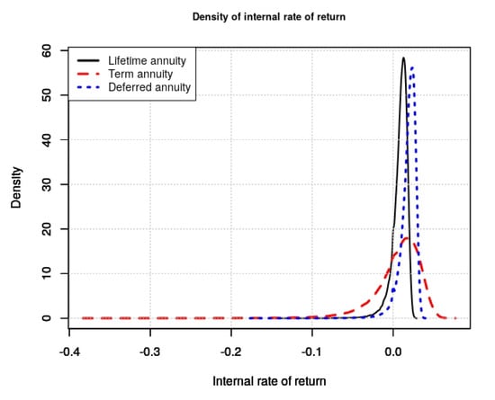
Figure 6.
Density of the internal rate of return for and .

Table 3.
Mean and Variance of the internal rates of return (IRRs) for the three annuities.
Based on the mean-variance criterion, it follows from Table 3 that at inception the deferred annuity using constant could yield higher IRR. But considering the variable , the comparison will depend on the level of the shareholder’s risk aversion, since he could decide not to invest an SC (referring to a deferred annuity) or to invest his SC on a lifetime annuity. As regards the term annuity, it seems to be less profitable, since it has the lower mean and the highest variance for a constant . Note that the values of the IRR for a deferred annuity using a variable confidence level cannot be computed, since the SC in this case is strictly negative.
From the observations on both the level of the annual benefits and the level of the SC, we can draw the following concluding remarks.
- (i)
- On the policyholder side, buying a term annuity will provide the annuitant with a good level of annual benefits but he will not be fully hedged against the longevity risk, whereas buying a deferred annuity will give a better level of annual benefits until death. In these cases, the longevity risk will partly be borne by the policyholders. The lifetime annuity gives the smallest level of annual benefits and fully hedges the annuitants against the longevity risk. Furthermore, for a fixed unique premium (respectively annual benefit), we can always find a pair of deferred time and term time such that the deferred and the term annuities provide the same annual benefits (respectively, the same unique premium). Note that combining successive term annuities could be a way to fully protect the annuitant against longevity risk, but in this case, the policyholder will face a pricing risk. The latter refers to the risk of rising annuity prices as a consequence of a high survival probability.
- (ii)
- On the insurer side, we can see that a positive SC is not always bad for an insurer, since it could yield a return even greater than a simple risk-free investment. Thus, the choice of the product to invest in depends on the risk aversion of the shareholders. Furthermore, identifying the product with the higher SC is subject to the computational time.
Even though we cannot draw up a strict comparison of these products by pointing out the best from both insurer and annuitant viewpoints, the results obtained here can be seen as a backing on which the two parties can base their choices.
5. Conclusions
The main goal of this paper was first to evaluate the level of the SC of an insurer with respect to some significant parameters for three different annuities (lifetime, deferred and term annuities), and secondly to draw up some comparative remarks from the obtained numerical results. This has been achieved within a single risk framework: the longevity risk framework where any other risk different from the longevity risk is assumed to be fully hedged. The built model is hence called the longevity model for which we used the HW process in order to model the force of mortality of the policyholders. Another main framework we based on is the SII framework where we consider the VaR as the (static) risk measure firstly with a constant confidence level of and secondly with a variable confidence level by .
From numerical analysis, we found that when the short rate increases, the SC decreases and the convex form obtained for the deferred annuity implies that there exists a computational time and a deferred period that minimizes the SC of the insurer. These results are some extensions of those obtained by Devolder and Lebègue (2017) wherein they considered a lump sum at retirement instead of series of payments. From the obtained results, we found that the choice of a product on the annuitant’s side strongly depends on annuitant’s expectations about their life time as well as on the level of benefit they could need. On the insurer side, the choice could depend on the level of the SC, but we also showed that providing a SC could yield quite good returns. The latter has been explained based on the mean-variance criterion of the internal rate of return of the three products. We also found that the SC computed with a constant confidence level of is much larger than the result obtained with a time-dependent confidence level. Moreover we observed that the term annuity does not fully hedge the annuitant against longevity risk, as the annuitant could still be alive after the end of the contract. In order to protect the policyholders against the longevity risk using term annuities, we could consider successive term annuities in future research.
In this model we only focused on the longevity risk measurement; additional risks (such as equity, interest rate and longevity risks) could be measured as well. Furthermore, we can think about using different risk measures, such as dynamic risk measures, and different mortality models and stochastic annual benefits. A more realistic and complete model will consist of considering market risks. All these generalized problems with unknown solutions constitute some open topics that could be subject to further research.
Author Contributions
P.M.N.D. and P.D. have equally contributed. All authors have read and agreed to the published version of the manuscript.
Funding
This research was funded by the UCLouvain-AG Insurance Chair.
Conflicts of Interest
The authors declare no conflict of interest.
Appendix A
Table A1 gives the values of the SC per unit of single premium for both immediate term and deferred annuities when both the deferred and the term times vary from 1 to 40. This is made using both constant and time-dependent confidence levels and at . We then observe that for the term annuity the value of the SC increases for small value of the term time and decreases for largest values of ; this is observed for both values of the confidence level. Regarding the deferred annuity, for variable confidence level, the SC strictly decreases for small values of the deferred time d and increases for larger value of d. Using the constant confidence level, we observe that the SC increases when d increases. Moreover, when the term time approaches 45, the value of the SC converges to the SC of a lifetime annuity (given by for constant and for variable ). When the deferred time d goes to 0, the value of the SC converges to the SC of a lifetime annuity.

Table A1.
Comparison of annuities for and .
Table A1.
Comparison of annuities for and .
| Term Annuity | Deferred Annuity | |||
|---|---|---|---|---|
| Values of and | Constant | Variable | Constant | Variable |
| 1 | 0.006156096 | 0.006153251 | 0.12403064 | 0.028944735 |
| 2 | 0.012352836 | 0.011125707 | 0.10912764 | 0.020232837 |
| 3 | 0.018453675 | 0.015353574 | 0.09544175 | 0.011929853 |
| 4 | 0.024303704 | 0.019543642 | 0.08413130 | 0.003968597 |
| 5 | 0.030369315 | 0.023229284 | 0.07259427 | −0.002910031 |
| 6 | 0.036514168 | 0.026574362 | 0.06354518 | −0.009368481 |
| 7 | 0.042701852 | 0.029546813 | 0.05693445 | −0.015076207 |
| 8 | 0.049113252 | 0.032413929 | 0.05428510 | −0.019060104 |
| 9 | 0.054907241 | 0.035345726 | 0.05368941 | −0.022470205 |
| 10 | 0.061024635 | 0.037834998 | 0.05721433 | −0.024729544 |
| 11 | 0.066085821 | 0.040194102 | 0.06270525 | −0.027540167 |
| 12 | 0.071862367 | 0.042155518 | 0.07390130 | −0.026949580 |
| 13 | 0.078535718 | 0.044084758 | 0.08444255 | −0.025193941 |
| 14 | 0.081923754 | 0.045936822 | 0.10052367 | −0.022804985 |
| 15 | 0.088126534 | 0.047274945 | 0.12330174 | −0.020479482 |
| 16 | 0.094834232 | 0.048906110 | 0.14671319 | −0.017047308 |
| 17 | 0.099364414 | 0.049970686 | 0.17094055 | −0.008042942 |
| 18 | 0.104767967 | 0.051177807 | 0.20153683 | −0.005249659 |
| 19 | 0.108327306 | 0.052016609 | 0.24425237 | 0.003488531 |
| 20 | 0.114894825 | 0.052853503 | 0.28521635 | 0.008879507 |
| 21 | 0.117501784 | 0.053364122 | 0.32288946 | 0.022371629 |
| 22 | 0.124528607 | 0.053879230 | 0.38329314 | 0.030489628 |
| 23 | 0.125890879 | 0.054244362 | 0.46111143 | 0.043680410 |
| 24 | 0.129962889 | 0.053597210 | 0.56054421 | 0.059427455 |
| 25 | 0.132918217 | 0.054048539 | 0.63835185 | 0.074547151 |
| 26 | 0.135450581 | 0.053696949 | 0.77494507 | 0.089206222 |
| 27 | 0.134558526 | 0.053324689 | 0.89920010 | 0.106217807 |
| 28 | 0.138901767 | 0.052551723 | 1.04882551 | 0.122351220 |
| 29 | 0.137323859 | 0.051922851 | 1.18591028 | 0.145081812 |
| 30 | 0.139340024 | 0.050700867 | 1.59980240 | 0.153899525 |
| 31 | 0.138424839 | 0.050212237 | 1.56913581 | 0.178013360 |
| 32 | 0.140725493 | 0.049092220 | 1.87843064 | 0.192808945 |
| 33 | 0.140501927 | 0.048290239 | 2.22641035 | 0.220370419 |
| 34 | 0.139830293 | 0.047356370 | 2.51850546 | 0.250856412 |
| 35 | 0.140390117 | 0.046204732 | 2.93846784 | 0.244808218 |
| 36 | 0.139532337 | 0.045694537 | 3.52777988 | 0.248769619 |
| 37 | 0.142093689 | 0.044263673 | 4.06141286 | 0.267697773 |
| 38 | 0.140524473 | 0.043942408 | 4.23378876 | 0.281096107 |
| 39 | 0.141067107 | 0.043023385 | 5.32838507 | 0.283869613 |
| 40 | 0.139819819 | 0.041877271 | 5.84001265 | 0.293670850 |
References
- Antolin, Pablo. 2007. Longevity Risk and Private Pensions. Available online: http://www.oecd.org/daf/fin/private-pensions/37977228.pdf (accessed on 25 May 2019).
- Antonio, Katrien, Lize Devolder, and Sander Devriendt. 2015. The IA| BE 2015 Mortality Projection for the Belgian Population. Available online: https://papers.ssrn.com/sol3/papers.cfm?abstract_id=2576167 (accessed on 15 March 2020).
- Barrieu, Pauline, Harry Bensusan, Nicole El Karoui, Caroline Hillairet, Stéphane Loisel, Claudia Ravanelli, and Yahia Salhi. 2012. Understanding, modelling and managing longevity risk: Key issues and main challenges. Scandinavian Actuarial Journal 3: 203–31. [Google Scholar] [CrossRef]
- Bauer, Daniel, Andreas Reuss, and Daniela Singer. 2012. On the calculation of the solvency capital requirement based on nested simulations. ASTIN Bulletin: The Journal of the IAA 42: 453–99. [Google Scholar]
- Bauer, Daniel, Daniela Bergmann, and Andreas Reuss. 2010. Solvency II and nested simulations: A least-squares Monte Carlo approach. Paper presented at 2010 ICA Congress, Sydney, Australia, 23–27 August 2010. [Google Scholar]
- Blake, David, and William Burrows. 2001. Survivor bonds: Helping to hedge mortality risk. Journal of Risk and Insurance 68: 339–48. [Google Scholar] [CrossRef]
- Brown, Jeffrey R., Olivia S. Mitchell, and James M. Poterba. 2000. National Bureau of Economic Research, Working Paper. Available online: https://www.nber.org/papers/w7812.pdf (accessed on 10 April 2019).
- Christiansen, Marcus C., and Andreas Niemeyer. 2014. Fundamental definition of the solvency capital requirement in solvency II. ASTIN Bulletin: The Journal of the IAA 44: 501–33. [Google Scholar] [CrossRef]
- Devineau, Laurent, and Stéphane Loisel. 2009. Risk aggregation in Solvency II: How to converge the approaches of the internal models and those of the standard formula? Bulletin Français d’Actuariat 9: 107–45. [Google Scholar]
- Devolder, Pierre, and Adrien Lebègue. 2017. Iterated VaR or CTE measures: A false good idea? Scandinavian Actuarial Journal 4: 287–318. [Google Scholar] [CrossRef]
- European Insurance and Occupational Pensions Authority. 2014a. Technical Specification for the Preparatory Phase (Part I). Available online: https://eiopa.europa.eu/Publications/ (accessed on 20 January 2018).
- European Insurance and Occupational Pensions Authority. 2014b. The Underlying Assumptions in the Standard Formula for the Solvency Capital Requirement Calculation. Available online: https://eiopa.europa.eu/Publications/ (accessed on 20 January 2018).
- Fung, Simon Man Chung, Katja Ignatieva, and Michael Sherris. 2019. Managing Systematic Mortality Risk in Life Annuities: An Application of Longevity Derivatives. Risks 7: 2. [Google Scholar] [CrossRef]
- Glasserman, Paul. 2013. Monte Carlo Method in Financial Engineering. New York: Springer Science and Business Media, vol. 53, p. 7. [Google Scholar]
- Gompertz, Benjamin. 1825. On the nature of the function expressive of the law of human mortality, and on a new mode of determining the value of life contingencies. Philosophical transactions of the Royal Society of London 115: 513–83. [Google Scholar]
- Gronchi, Sandro. 1986. On investment criteria based on the internal rate of return. Oxford Economic Papers 38: 174–80. [Google Scholar] [CrossRef]
- Hainaut, Donatien, Pierre Devolder, and Antoon Pelsser. 2007. Robust evaluation of SCR for participating life insurances under Solvency II. Insurance: Mathematics and Economics 79: 107–23. [Google Scholar] [CrossRef]
- Hari, Norbert, Anja De Waegenaere, Bertrand Melenberg, and Theo E. Nijman. 2008. Longevity risk in portfolios of pension annuities. Insurance: Mathematics and Economics 42: 505–19. [Google Scholar] [CrossRef]
- Kochanski, Michael, and Bertel Karnarski. 2011. Solvency capital requirement for hybrid products. European Actuarial Journal 1: 173–98. [Google Scholar] [CrossRef]
- Lichters, Roland, Roland Stamm, and Donal Gallagher. 2015. Hull-White Model. In Modern Derivatives Pricing and Credit Exposure Analysis. New York: Springer, pp. 403–22. [Google Scholar]
- Liebwein, Peter. 2006. Risk models for capital adequacy: Applications in the context of solvency II and beyond. The Geneva Papers on Risk and Insurance-Issues and Practice 31: 528–50. [Google Scholar] [CrossRef]
- Ng, Andrew Cheuk-Yin, and Johnny Siu-Hang Li. 2011. Valuing variable annuity guarantees with the multivariate Esscher transform. Insurance: Mathematics and Economics 49: 393–400. [Google Scholar] [CrossRef]
- Ohlsson, Esbjörn, and Jan Lauzeningks. 2009. The one-year non-life insurance risk. Insurance: Mathematics and Economics 45: 203–208. [Google Scholar] [CrossRef]
- Olivieri, Annamaria, and Ermanno Pitacco. 2008. Solvency Requirements for Life Annuities: Some Comparisons. Working Paper. Available online: http://ssrn.com/abstract=1266094 (accessed on 15 June 2019).
- Pfeifer, Dietmar, and Doreen Strassburger. 2008. Solvency II: stability problems with the SCR aggregation formula. Scandinavian Actuarial Journal 2: 61–77. [Google Scholar] [CrossRef]
- Vasicek, Oldrich A., and H. Gifford Fong. 2015. Term structure modeling using exponential splines. In Finance, Economics, and Mathematics. New York: John Wiley & Sons. [Google Scholar]
- Zeddouk, Fadoua, and Pierre Devolder. 2019. Mean Reversion in Stochastic Mortality: Why and How? ISBA Discussion Paper, UClouvain. Available online: http://hdl.handle.net/2078.1/219343 (accessed on 20 January 2020).
© 2020 by the authors. Licensee MDPI, Basel, Switzerland. This article is an open access article distributed under the terms and conditions of the Creative Commons Attribution (CC BY) license (http://creativecommons.org/licenses/by/4.0/).

