Implementing the Rearrangement Algorithm: An Example from Computational Risk Management


Department of Statistics and Actuarial Science, University of Waterloo, 200 University Avenue West, Waterloo, ON N2L 3G1, Canada
Risks 2020, 8(2), 47; https://doi.org/10.3390/risks8020047
Submission received: 20 April 2020
/
Revised: 8 May 2020
/
Accepted: 8 May 2020
/
Published: 14 May 2020
(This article belongs to the Special Issue Computational Risk Management)
Abstract
:After a brief overview of aspects of computational risk management, the implementation of the rearrangement algorithm in R is considered as an example from computational risk management practice. This algorithm is used to compute the largest quantile (worst value-at-risk) of the sum of the components of a random vector with specified marginal distributions. It is demonstrated how a basic implementation of the rearrangement algorithm can gradually be improved to provide a fast and reliable computational solution to the problem of computing worst value-at-risk. Besides a running example, an example based on real-life data is considered. Bootstrap confidence intervals for the worst value-at-risk as well as a basic worst value-at-risk allocation principle are introduced. The paper concludes with selected lessons learned from this experience.
1. Introduction
Computational risk management is a comparably new and exciting field of research at the intersection of statistics, computer science and data science. It is concerned with computational problems of quantitative risk management, such as algorithms, their implementation, computability, numerical robustness, parallel computing, pitfalls in simulations, run-time optimization, software development and maintenance. At the end of the (business) day, solutions in quantitative risk management are to be run on a computer of some sort and thus concern computational risk management.
There are various factors that can play a role when developing and implementing a solution to a problem from computational risk management in practice, for example:
- (1)
- Theoretical hurdles. Some solutions cannot be treated analytically anymore. Suppose is a d-dimensional random vector of risk factor changes, for example negative log-returns, with marginal distribution functions and we are interested in computing the probability of the jth risk factor change to take on values between its - and its -quantile for all j. Even if we knew the joint distribution function H of , computing such a probability analytically involves evaluating H at different values. For , this can already be time-consuming (not to speak of numerical inaccuracies appearing, which render the formula as good as useless) and for the number of points at which to evaluate H is roughly equal to the estimated number of atoms in the universe.
- (2)
- Model risk. The risk of using the wrong model or a model in which assumptions are not fulfilled; every solution we implement is affected by model risk to some degree. In the aforementioned example, not knowing the exact H leads to model risk when computing the given probability by Monte Carlo integration.
- (3)
- The choice of software. The risk of using the wrong software; in the above example, a software not suitable for simulating from joint distribution functions H. Another example is to use a programming language too low-level for the problem at hand, requiring to implement standard tasks (sampling, optimization, etc.) manually and thus bearing the risk of obtaining unreliable results because of many possible pitfalls one might encounter when developing the tools needed to implement the full-blown solution. These aspects become more crucial nowadays since efficient solutions to different problems are often only available in one software each but companies need to combine these solutions and thus the corresponding software in order to solve these different problems at hand.
- (4)
- Syntax errors. These are compilation errors or execution errors by an interpreter because of a violation of the syntax of the programming language under consideration. Syntax errors are typically easy to detect as the program simply stops to run. Also, many programming languages provide tools for debugging to find the culprits.
- (5)
- Run-time errors. These are errors that appear while a program runs. Quite often, run-time errors are numerical errors, errors that appear, for example, because of the floating-point representation of numbers in double precision. Run-time errors can sometimes be challenging to find, for example, when they only happen occasionally in a large-scale simulation study and introduce a non-suspicious bias in the results. Run-time errors can sometimes also be hard to reproduce.
- (6)
- Semantic errors. These are errors where the code is syntactically correct and the program runs, but it does not compute what is intended (for example, due to a flipped logical statement). If results do not look suspicious or pass all tests conducted, sometimes measuring run time can be the only way to find such problems (for example, if a program finishes much earlier than expected).
- (7)
- Scaling errors. These are errors of an otherwise perfectly fine running code that fails when run at large scale. This could be due to a lack of numerical robustness, the sheer run time of the code, an exploding number of parameters involved, etc.
- (8)
- User errors. These are errors caused by users of the software solution; for example, when calling functions with wrong arguments because of a misinterpretation of their meaning. The associated risk of wrongly using software can, by definition, often be viewed as part of operational risk.
- (9)
- Warnings. Warnings are important signs of what to watch out for; for example, a warning could indicate that a numerical optimization routine has not converged after a predetermined number of steps and only the current best value is returned, which might be far off a local or the global optimum. Unfortunately, especially in large-scale simulation studies, users often suppress warnings instead of collecting and considering them.
- (10)
- Run time. The risk of using or propagating method A over B because the run time of A beats the one of B by a split second or second, not realizing that run time depends on factors such as the hardware used, the current workload, the algorithm implemented, the programming language used, the implementation style, compiler flags, whether garbage collection was used, etc. There is not even a unique concept of time (system vs. user vs. elapsed time).
- (11)
- Development and maintenance. It is significantly more challenging to provide a robust, well developed, maintained and documented class of solutions as part of a bigger, coherent software package rather than a single script with hard-coded values to solve a special case of the same problem. Although stand-alone scripts get specific tasks done by 4 p.m., having a software package available is typically beneficial mid- to long-term. It can significantly reduce the risk of the aforementioned errors by reusing code well tested and applied by the users of the package or it can avoid the temptation of introducing errors long after the code was developed just because it suddenly looks suspicious although it is actually correct.
At the core of all solutions to problems from computational risk management lies an algorithm, a well-defined (unambiguous) finite set of instructions (steps) for solving a problem. An implementation of an algorithm in a programming language allows one to see how a problem is actually solved, unlike a formulation in pseudo-code, which is often vague and thus opens the door for misinterpretation. A classical example is if pseudo-code says “Minimize the function…” without mentioning how initial values or intervals can be obtained. Another example is “Choose a tolerance …” but one is left in the dark concerning what suitable tolerances are for the problem at hand; they often depend on the unknown output one is interested to compute in the first place, see Step (1) of Algorithm 1 later. Oftentimes, these are the hardest parts to solve of the whole problem and it is important for research and scientific journals to accept corresponding contributions as important instead of brushing them off as “not innovative” or representing “no new contribution”.
A fundamental principle when developing an implementation is that of a minimal working example. A minimal working example is source code that is a working example in the sense that it allows someone else to reproduce a problem (sufficiency) and it is minimal in the sense that it is as small and as simple as possible, without non-relevant code, data or dependencies (necessity). Minimal working examples are often constructed from existing larger chunks of code by divide and conquer, that is by breaking down the problem into sub-problems and commenting out non-relevant parts until the code becomes simple enough to show the problem (which is then easier to grasp and solve or can be sent to an expert in the field to ask for help).
In this paper, we consider the problem of implementing the rearrangement algorithm (RA) of Embrechts et al. (2013) as an example from computational risk management. The RA allows one to compute, for example, the worst value-at-risk of the sum of d risks of which the marginal distributions are known but the dependence is unknown; it can also be used to compute the best value-at-risk or expected shortfall, but we focus on the worst value-at-risk. Section 2 contains the necessary details about the RA. Section 3 addresses how the major workhorse underlying this algorithm can be implemented in a straightforward way in R. This turns out to be inefficient and Section 4 presents ways to improve the implementation. Section 5 utilizes the implementations in our R package for tracing and to motivate the chosen default tolerances, and Section 6 considers a real data example, presents a bootstrap confidence interval for worst value-at-risk and introduces a basic capital allocation principle based on worst value-at-risk. The lessons learned throughout the paper are summarized in Section 7.
2. The Rearrangement Algorithm in a Nutshell
Let be continuously distributed loss random variables over a predetermined period and let be the total loss over that time period. From a risk management perspective we are interested in computing value-at-risk (, or VaR) at confidence level , that is the -quantile of the distribution function of ; in typical applications, . If we had enough joint observations, so realizations of the random vector , we could estimate empirically. A major problem is that one often only has realizations of each of individually, non-synchronized. This typically allows to pin down but not the joint distribution function H of . By Sklar’s Theorem, such H can be written as
for a unique copula C. In other words, although we often know or can estimate , we typically neither know the copula C nor have enough joint realizations to be able to estimate it. However, the copula C determines the dependence between and thus the distribution of as the following example shows.
Example 1 ![Risks 08 00047 i001]()
![Risks 08 00047 i002]()
![Risks 08 00047 i003]()
(Motivation for rearrangements).
Consider and , , , that is both losses are Pareto Type I distributed with parameter . The left-hand side of Figure 1 shows realizations of , once under independence, so for , and once under comonotonicity, so for . We see that the different dependence structures directly influence the shape of the realizations of .

As the middle of Figure 1 shows, the dependence also affects . This example is chosen to be rather extreme, (perhaps) in (stark) contrast to intuition, under independence is even larger than under comonotonicity, for all α; this can also be shown analytically in this case in a rather tedious calculation; see (Hofert et al. 2020, Exercise 2.28).

The right-hand side of Figure 1 shows the same plot with the marginal distributions now being gamma. In this case, comonotonicity leads to larger values of than independence, but only for sufficiently large α; the corresponding turning point seems to get larger the smaller the shape parameter of the second margin, for example.

Note that we did not utilize the stochastic representation , , for sampling . Instead, we sorted the realizations of so that their ranks are aligned with those of , in other words, so that the ith-smallest realization of lies next to the ith-smallest realizations of . The rows of this sample thus consist of , where denotes the ith order statistic of the n realizations of . Such a rearrangement mimics comonotonicity between the realizations of and . Note that this did not change the realizations of or individually, so it did not change the marginal realizations, only the joint ones.
As we learned from Example 1, by rearranging the marginal loss realizations, we can mimic different dependence structures between the losses and thus influence . In practice, the worst , denoted by , is of interest, that is the largest for given margins . The following remark motivates an objective when rearranging marginal loss realizations in order to increase and thus approximate .
Remark 1
(Objective of rearrangements).
- (1)
- By Example 1, the question which copula C maximizes is thus, at least approximately, the question of which reordering of realizations of each of leads to . For any C, the probability of exceeding is (at most, but for simplicity let us assume exactly) . How that probability mass is distributed beyond depends on C. If we find a C such that has a rather small variance , more probability mass will be concentrated around a single point which can help to pull further into the right tail and thus increase ; Figure 2 provides a sketch in terms of a skewed density. If that single point exists and if , then it must be expected shortfall, which provides an upper bound to .
- (2)
- It becomes apparent from Figure 2 that the distribution of below its α-quantile is irrelevant for the location of . It thus suffices to consider losses beyond their marginal α-quantiles , so the conditional losses , , and their copula , called worst VaR copula. Note that since α is typically rather close to 1, the distribution of (the tail of ) is typically modeled by a continuous distribution; this can be justified theoretically by the Pickands–Balkema–de-Haan Theorem, see (McNeil et al. 2015, Section 5.2.1).
- (3)
- In general, if cannot be attained, the smallest point of the support of given that , , is taken as an approximation to .
The RA aims to compute by rearranging realizations of , , such that their sum becomes more and more constant, in order to approximately obtain the smallest possible variance and thus the largest . There are still fundamental open mathematical questions concerning the convergence of this algorithm, but this intuition is sufficient for us to understand the RA and to study its implementation. To this end, we now address the remaining underlying concepts we need.
For each margin , the RA uses two discretizations of beyond the probability as realizations of to be rearranged. In practice, one would typically utilize the available data from to estimate its distribution function and then use the implied quantile function of the fitted to obtain such discretizations; see Section 6. Alternatively, could be specified by expert opinion. The RA uses two discretizations to obtain upper and lower bounds to , which, when sufficiently close, can be used to obtain an estimate of , for example, by taking the midpoint. The two discretizations are stored in the matrices
These matrices are the central objects the RA works with. For simplicity of the argument, we write if the argument applies to or . The RA iterates over the columns of and successively rearranges each column in a way such that the row sums of the rearranged matrix have a smaller variance; compare with Remark 1.
In each rearrangement step, the RA rearranges the jth column of oppositely to the vector of row sums of all other columns, where . Two vectors and are called oppositely ordered if for all . After oppositely ordering, the (second-, third-, etc.) smallest component of lies next to the (second-, third-, etc.) largest of , which helps decrease the variance of their componentwise sum. To illustrate this, consider the following example.
Example 2 ![Risks 08 00047 i004]()
![Risks 08 00047 i005]()
![Risks 08 00047 i006]()
![Risks 08 00047 i007]()
![Risks 08 00047 i008]()
(Motivation for oppositely ordering columns).
We start by writing an auxiliary function to compute a matrix with the modification that for , 1-quantiles appearing in the last row are replaced by to avoid possible infinities; we come back to this point later. It is useful to start writing functions at this point, as we can reuse them later and rely on them for computing partial results, inputs needed, etc. In R, the function can be used to check inputs of functions. If any of the provided conditions fails, this would produce an error. For more elaborate error messages, one can work with . Input checks are extremely important when functions are exported in a package (so visible to a user of the package) or even made available to users by simply sharing R scripts. Code is often run by users who are not experts in the underlying theory or mechanisms and good input checks can prevent them from wrongly using the shared software; see Section 1 Point (8). Also, documenting the function (here: Roxygen-style documentation) is important, providing easy to understand information about what the function computes, meaning of input parameters, return value and who wrote the function.

Consider and , , , that is each of the two losses is Pareto distributed; we choose and here. We start by building the list of marginal quantile functions and then compute the corresponding (here: upper) quantile matrix for and .

The columns in are sorted in increasing order, so mimic comonotonicity in the joint tail, which leads to the following variance estimate of the row sums.

If we randomly shuffle the first column, so mimicking independence in the joint tail, we obtain the following variance estimate.

Now if we oppositely order the first column with respect to the sum of all others, here the second column, we can see that the variance of the resulting row sums will decrease; note that we mimic countermonotonicity in the joint tail in this case.

The two marginal distributions largely differ in their heavy-tailedness, which is why the variance of their sum, even when oppositely reordered is still rather large. For , one obtains , for two standard normal margins and for two standard uniform distributions 0.
As a last underlying concept, the RA utilizes the minimal row sum operator
which is motivated in Remark 1 Part (3). We are now ready to provide the RA.
The RA as introduced in Embrechts et al. (2013) states that and in practice . Furthermore, the initial randomizations in Steps (2.2) and (3.2) are introduced to avoid convergence problems of .
3. A First Implementation of the Basic Rearrangement Step
When implementing an algorithm such as the RA, it is typically a good idea to divide and conquer, which means breaking down the problem into sub-problems and addressing those first. Having implemented solutions to the sub-problems (write functions!), one can then use them as black boxes to implement the whole algorithm. In our case, we can already rely on the function for Steps (2.1) and (3.1) of the RA and we have already seen how to oppositely order two columns in Example 2. We also see that apart from which matrix is rearranged, Steps (2) and (3) are equal. We thus focus on this step in what follows.
Example 3 ![Risks 08 00047 i009]()
(Basic rearrangements).
We start with a basic implementation for computing one of the bounds of the RA.

In comparison to Algorithm 1, our basic implementation already uses a relative rather than an absolute convergence tolerance ε (more intuitively named in our implementation), the former is more suitable here as we do not know and therefore cannot judge whether an absolute tolerance of, say, is reasonable. Also, we terminate if the attained relative tolerance is less than or equal to since including equality allows us to choose ; see Steps (2.4) and (3.4) of Algorithm 1. Furthermore, we allow the tolerance to be in which case the columns are rearranged until all of them are oppositely ordered with respect to the sum of all other. The choice is good for testing, but typically results in much larger run times and rarely has an advantage over .
| Algorithm 1: Rearrangement algorithm for computing bounds on |
|
The opposite ordering step in our basic implementation contains the argument of , which specifies how ties are handled, namely those ties with smaller index get assigned the smaller rank. Although this was not a problem in Example 2, when N is large and , ties can quickly arise numerically. It can be important to use a sorting algorithm that has deterministic behavior in this case, as otherwise, the RA might not terminate or not as quickly as it could; see the vignette of the Rpackage for more details.
Finally, we can call on both matrices in Equation (1) to obtain the lower and upper bounds , and thus implement the RA. We would thus reuse the same code for Steps (2) and (3) of the RA, which means less code to check, improve or maintain.
Example 4 ![Risks 08 00047 i010]()
![Risks 08 00047 i011]()
(Using the basic implementation).
To call in a running example, we use the following parameters and build the input matrix .

We can now call and also measure the elapsed time in seconds of this call.

4. Improvements
It is always good to have a first working version of an algorithm, for example, to compare against in case one tries to improve the code and it becomes harder to read or check. However, as we saw in Example 4, our basic implementation of Example 3 is rather slow even if we chose a rather small N in this running example. Our goal is thus to present ideas how to improve as a building block of the RA.
4.1. Profiling
As a first step, we profile the last call to see where most of the run time is spent.

Profiling writes out the call stack every so-many split seconds, so checks where the execution currently is. This allows one to measure the time spent in each function call. Note that some functions do not create stack frame records and thus do not show up. Nevertheless, profiling the code is often helpful. It is typically easiest to consider the measurement in percentage (see second and fourth column in the above output) and often in total, so the run time spent in that particular function or the functions it calls (see the fourth column). As this column reveals, two large contributors to run time are the computation of row sums and the sorting.
4.2. Avoiding Summations
First consider the computation of row sums. In each rearrangement step, computes the row sums of all but the current column. As we explained, this rearrangement step is mathematically intuitive but it is computationally expensive. An important observation is that the row sums of all but the current column is simply the row sums of all columns minus the current column; in short, . Therefore, if we, after randomly permuting each column, compute the total row sum once, we can subtract the jth column to obtain the row sums of all but the jth column. After having rearranged the jth column, we then add the rearranged jth column to the row sums of all other columns in order to obtain the updated total row sums.
Example 5 ![Risks 08 00047 i013]()
![Risks 08 00047 i014]()
![Risks 08 00047 i015]()
(Improved rearrangements).
The following improved version of incorporates said idea; to save space, we omit the function header.

Next, we compare with . We check if we obtain the same result and also measure run time as a comparison.

Run time is substantially improved by about 85%. This should be especially helpful for large d, so let us investigate the percentage improvement; here only done for rather small d to show the effect. Figure 3 shows the relative speed-up in percentage of over as a function of d for the running example introduced in Example 4.

We can infer that the percentage improvement of in comparison to converges to 100% for large d. This is not a surprise since determining the row sums of all but a fixed column requires to compute -many sums whereas requires only N-many. This is an improvement by , which especially starts to matter for large d.
A quick note on run-time measurement is in order here. In a more serious setup, one would take repeated measurements of run time (at least for smaller d), determine the average run time for each d and perhaps empirical confidence intervals for the true run time based on the repeated measurements. Also, we use the same seed for each method, which guarantees the same shuffling of columns and thus allows for a fair comparison. Not doing so can result in quite different run times and would thus indeed require repeated measurements to get more reliable results.
Finally, the trick of subtracting a single column from the total row sums in order to obtain the row sums of all other columns comes at a price. Although the RA as in Algorithm 1 works well if some of the 1-quantiles appearing in the last row of are infinity, this does not apply to anymore since if the last entry in the jth column is infinity, the last entry in the vector of total row sums is infinity and thus the last entry in the vector of row sums of all but the jth column would not be defined ( in R). This is why avoids computing 1-quantiles; see Example 2.
4.3. Avoiding Accessing Matrix Columns and Improved Sorting
There are two further improvements we can consider.
The first concerns the opposite ordering of columns. It so far involved a call to and one to . It turns out that these two calls can be replaced by a nested call, which is slightly faster than alone. We start by demonstrating that we can replicate by a nested call based on standard uniform data.

Providing with a method to deal with ties is important here as the default assigns average ranks on ties and thus can produce non-integer numbers. One would not guess to see ties in such a small set of standard uniform random numbers, but that is not true; see Hofert (2020) for details.
To see how much faster the nested call is than , we consider a small simulation study. For each of the two methods, we measure elapsed time in seconds when applied 20 times to samples of random numbers of different sizes.

Figure 4 provides a summary in terms of a box plot. We see that the nested call is faster than ; percentages by how much the latter is worse are displayed in the labels.

As a second improvement, recall that the RA naturally works on the columns of matrices. Matrices or arrays are internally stored as long vectors with attributes indicating when to “wrap around”. Accessing a matrix column thus requires to determine the beginning and the end of that column in the flattened vector. We can thus speed-up by working with lists of columns instead of matrices.
The following example incorporates these two further improvements and some more.
Example 6 ![Risks 08 00047 i019]()
![Risks 08 00047 i020]()
(Advanced rearrangements).
The following implementation saves column-access time by working with lists rather than matrices. We also use the slightly faster (as we know the dimensions of the input matrix) instead of for computing the initial row sums once in the beginning, and we incorporate the idea of a nested call instead of . Furthermore, before shuffling the columns, we also store their original sorted versions, which allows us to omit the call of in .

We now check for correctness of and measure its run time in our running example. Concerning correctness, for the more involved it is especially useful to have simpler versions available to check against; we use the result of here as we already checked it, but could have equally well used the one of .

Although the gain in run time is not as dramatic as before, we still see an improvement of about 62% in comparison to .
4.4. Comparison with the Actual Implementation
The computational improvements so far have already lead to a percentage improvement of 94% in comparison to in our running example. The following example compares our fastest function so far with our implementation in the R package whose development was motivated by a risk management team at a Swiss bank.
Example 7 ![Risks 08 00047 i021]()
![Risks 08 00047 i022]()
(Comparison withrearrange().)
To save even more run time, the function from the Rpackage splits the input matrix into its columns at C level. It also uses an early stopping criterion in the sense that after all columns have been rearranged once, stopping is checked after every column rearrangement. Because of the latter, the result is not quite comparable to our previous versions.

We did not measure run time here since, similar to Heisenberg’s uncertainty principle, the difference in run time becomes more and more random; this is in line with the point we made about run-time measurement in the introduction. In other words, the two implementations become closer in run time. This can be demonstrated by repeated measurements.

As we see from the box plot in Figure 5, on average, is slightly faster than . Although could even be made faster, it also computes and returns more information about the rearrangements than ; for example, the computed minimal row sums after each column rearrangement and the row of the final rearranged matrix corresponding to the minimal row sum in our case here. Given that this is a function applied by users who are not necessarily familiar with the rearrangement algorithm, it is more important to provide such information. Nevertheless, is still faster than on average.
The function is the workhorse underlying the function that implements the rearrangement algorithm in the R package . The adaptive rearrangement algorithm (ARA) introduced in Hofert et al. (2017) improves the RA in that it introduces the joint tolerance, that is the tolerance between and ; the tolerance used so far is called individual tolerance. The ARA applies column rearrangements until the individual tolerance is met for each of the two bounds and until the joint tolerance is met or a maximal number of column rearrangements has been reached. If the latter is the case, N is increased and the procedure repeated. The ARA implementation in also returns useful information about how the algorithm proceeded. Overall, neither requires to choose a tolerance nor the number of discretization points, which makes this algorithm straightforward to apply in practice where the choice of such tuning parameters is often unclear. Finding good tuning parameters (adaptively or not) is often a significant problem in newly suggested procedures and not rarely a question open for future research by itself.
5. The Functions and
In this section we utilize the implementations and of the rearrangement step and the adaptive rearrangement algorithm.
Example 8 ![Risks 08 00047 i023]()
(Tracingrearrange().)
The implementation has a tracing feature. It can produce a lot of output but we here consider the rather minimal example of rearranging the matrix
The following code enables tracing () to see how the column rearrangements proceed; to this end we rearrange until all columns are oppositely ordered to the sum of all other columns (), disable random permutation of the columns () and provide the information that the columns are already sorted here ().

A “|” or “=” symbol over the just worked on column indicates whether this column was changed (“|”) or not (“=”) in this rearrangement step. The last two printed columns provide the row sums of all other columns as well as the new updated total row sums after the rearrangement. As we can see from this example, the rearranged matrix has minimal row sum 5 and is given by
would have led to the larger minimal row sum 6; this rather constructed example for when the greedy column rearrangements of the RA can fail to provide the maximal minimal row sum was provided by Haus (2015). As more interesting example to trace is to rearrange the matrix
see the vignette of the Rpackage .
Example 9 ![Risks 08 00047 i024]()
![Risks 08 00047 i025]()
![Risks 08 00047 i026]()
(CallingARA())
We now call in the case of our running example in this paper.

As we can see, the implementation returns a list with the computed bounds , the relative rearrangement gap , the two individual and one joint tolerance reached on stopping, a corresponding vector of logicals indicating whether the required tolerances have been met, the number N of discretization points used in the final step, the number of considered column rearrangements for each bound, vectors of computed optimal (for worst VaR this means “minimal”) row sums after each column rearrangement considered, a list with the two input matrices , a list with the corresponding final rearranged matrices and the rows corresponding to their optimal row sums. An estimate of in our running example can then be computed as follows.

Figure 6 shows the minimal row sum as a function of the number of rearranged columns for each of the two bounds and on in our running example. We can see that already after all columns were rearranged once, the actual value of the two bounds does not change much anymore in this case, yet the algorithm still proceeds until the required tolerances are met.

6. Applications
We now consider a real data example and introduce bootstrap confidence intervals for as well as a basic worst VaR allocation principle.
Example 10 ![Risks 08 00047 i027]()
![Risks 08 00047 i028]()
![Risks 08 00047 i029]()
![Risks 08 00047 i030]()
![Risks 08 00047 i031]()
![Risks 08 00047 i032]()
![Risks 08 00047 i033]()
(A real-life example).
We consider negative log-returns of Google, Apple and Microsoft stocks from 2006-01-03 to 2010-12-31.

We treat the negative log-returns as (roughly) stationary here and consider mean excess plots in Figure 7 to determine suitable thresholds for applying the peaks-over-threshold method.

We then fit generalized Pareto distributions (GPDs) to the excess losses over these thresholds.

We consider the corresponding quantile functions as approximate quantile functions to our empirical losses; see (McNeil et al. 2015, Section 5.2.3).

Based on these quantile functions, we can then compute with .

Given the additional information obtained from , we can also visualize a (pseudo-)sample from the worst VaR copula , see Figure 8. Such a sample is obtained by computing the pseudo-observations, that is componentwise ranks scaled to , of the rearranged matrix corresponding to the upper bound ; we could have also considered here.

Also, we can investigate how much the bounds and change with changing individual relative tolerance. Figure 9 motivates the use of 0 as individual relative tolerance; this is often quite a bit faster than and provides similar bounds.

Example 11 ![Risks 08 00047 i034]()
![Risks 08 00047 i035]()
![Risks 08 00047 i036]()
![Risks 08 00047 i037]()
![Risks 08 00047 i038]()
(Bootstrap confidence interval for worst VaR).
As in Example 10 and mentioned in Section 2, the marginal quantile functions used as input for the rearrangement algorithm may need to be estimated from data. The corresponding estimation error translates to a confidence interval for , which we can obtain from a bootstrap. To this end, we start by building B bootstrap samples from the negative log-returns; we choose a rather small here to demonstrate the idea.

Next, we build excess losses over 90% thresholds (a typical broad-brush choice in practice), fit GPDs to the d component samples for each of the B bootstrap samples and construct the corresponding quantile functions.

Now we can call with each of the B sets of marginal quantile functions.

And then extract the computed estimates of .

A bootstrap 95%-confidence interval for is thus given as follows.

Note that our run-time improvements of Section 4 are especially useful here as a bootstrap would otherwise be relatively time-consuming.
Example 12 ![Risks 08 00047 i039]()
![Risks 08 00047 i040]()
![Risks 08 00047 i041]()
(Basic worst VaR allocation).
Capital allocation concerns the allocation of a total capital K to d business lines so that (the full allocation property), where denotes the capital allocated to business line j. As the RA uses the minimal row sum as estimate, the rows in the final rearranged matrices provide an allocation of one can call worst VaR allocation. There could be multiple rows in leading to the minimal row sum in which case the componentwise average of these rows is considered. The resulting two rows are returned by ( and) in version . By componentwise averaging, the latter two rows we obtain an approximate worst VaR allocation. Given that we already have a bootstrap sample, we can average the B computed allocations componentwise to obtain the bootstrap mean of the worst VaR allocation.

We can also compare the corresponding estimate of the total allocation with the average of the B optimal row sums computed by the ARA to check the full allocation property; to this end, we first compute the B averages of the optimal row sums over the lower and upper bounds for each replication.

Bootstrap 95%-confidence intervals for each of can be obtained as follows.

For other applications of the RA, see, for example, Embrechts and Jakobsons (2016), Bernard et al. (2017), Bernard et al. (2018) and, most notably, Ramsey and Goodwin (2019) where the RA is applied in the context of crop insurance.
7. Selected Lessons Learned
After using R to motivate column rearrangements and opposite ordering for finding the worst VaR for given marginal distributions in Section 2, we considered a basic implementation of such rearrangement in Section 3. We profiled the code in Section 4 and improved the implementation step-by-step by avoiding unnecessary summations, avoiding accessing matrix columns and improving the sorting step. In Section 5 we then used the implementations and in our R package to trace the rearrangement steps and to motivate the use of the default tolerances used by . A real data example was considered throughout Section 6 where we computed the worst VaR with , visualized a sample from the corresponding worst VaR copula and assessed the sensitivity of the computed worst VaR with respect to the individual convergence tolerance. To incorporate the uncertainty due to the estimation error of the marginal distributions, we used a bootstrap idea to obtain a confidence interval for the true worst VaR. We also introduced worst VaR allocation as a capital allocation principle and computed bootstrap confidence intervals for the allocated capitals.
Our experiments reveal lessons to learn that frequently appear in problems from the realm of computational risk management:
- ■
- We can and should use software to learn about new problems and communicate their solutions. Implementing an algorithm often helps to fully comprehend a problem, experiment with it and get new ideas for practical solutions. It also allows one to communicate a solution since an implementation is unambiguous even if a theoretical presentation or pseudo-code of an algorithm leaves questions unanswered (such as how to choose tuning parameters); the latter is often the case when algorithms are provided in academic research papers.
- ■
- Both for understanding a problem and for communicating its solution, it is paramount to use visualizations. Creating meaningful graphs is unfortunately still an exception rather than the rule in academic publications where tables are frequently used. Tables mainly allow one to see single numbers at a time, whereas graphs allow one to see the “bigger picture”, so how results are connected and behave as functions of the investigated inputs.
- ■
- Given an algorithm, start with a basic, straightforward implementation and make sure it is valid, ideally by testing against known solutions in special cases; we omitted that part here, but note that there are semi-analytical solutions available for computing worst VaR in the case of homogeneous margins.
- ■
- Learn from the basic implementation, experiment with it and improve it, for example, by improving numerical stability, run time, maintenance, etc. If you run into problems along the way, use minimal working examples to solve them; they are typically constructed by divide and conquer. As implementations get more involved, compare them against the basic implementation or previously checked improved versions.
- ■
- When improving code, be aware of the issues mentioned in the introduction and exploit the fact that mathematically unique solutions often allow for different computational solutions. Also, computational problems (ties, parts of domains close to limits, etc.) can arise when there are none mathematically. These are often the hardest problems to solve, which is why it is important to be aware of computational risk management problems and their solutions. Implementing a computationally tractable solution is often one “dimension” more complicated than finding a mathematical solution—also literally, since a random variable (random vector) is often replaced by a vector (matrix) of realizations in a computational solution.
- ■
- Results in academic research papers are often based on an implementation of a newly presented algorithm that works only under specific conditions with parameters found by experimentation (often hard-coded) under such conditions in the examples considered. A publicly available implementation in a software package needs to go well beyond this point; for example, as users typically do not have expert knowledge of problems the implementation intends to solve and often come from different backgrounds altogether in the hope to find solutions to challenging problems in their field of application. On the one hand, the amount of work spent on development and maintenance of publicly available software solutions is largely underestimated. On the other hand, one can sometimes benefit from getting to know different areas of application or valuable input for further theoretical or computational investigation through user feedback. Also, ones own implementation often helps one to explore potential further improvements or new solutions altogether.
- ■
- Optimizing run time to be able to apply solutions in practical situations can be important but is not all there is. Providing a readable, comprehensible and numerically stable solution is equally important, for example. Code optimized solely for run time typically becomes less transparent and harder to maintain, is thus harder to adapt to future conceptual improvements and more prone to semantic errors. Also, a good solution typically not only provides a final answer but useful by-products and intermediate results computed along the way, just like a good solution in a mathematical exam requires intermediate steps to be presented in order to obtain full marks (which also simplifies to find the culprit if the final answer is erroneous).
Funding
This research was funded by NSERC under Discovery Grant RGPIN-5010-2015.
Acknowledgments
The author would like to thank Kurt Hornik (Wirtschaftsuniversität Wien) and Takaaki Koike (University of Waterloo) for valuable feedback and inspiring discussions.
Conflicts of Interest
The author declares no conflict of interest.
Abbreviations
The following abbreviations are used in this manuscript:
| ARA | adaptive rearrangement algorithm |
| RA | rearrangement algorithm |
| VaR | value-at-risk |
References
- Bernard, Carole, Michel Denuit, and Steven Vanduffel. 2018. Measuring portfolio risk under partial dependence information. The Journal of Risk and Insurance 85: 843–63. [Google Scholar] [CrossRef] [Green Version]
- Bernard, Carole, Ludger Rüschendorf, Steven Vanduffel, and Jing Yao. 2017. How robust is the value-at-risk of credit risk portfolios? The European Journal of Finance 23: 507–34. [Google Scholar] [CrossRef]
- Embrechts, Paul, and Edgars Jakobsons. 2016. Dependence uncertainty for aggregate risk: Examples and simple bounds. In The Fascination of Probability, Statistics and Their Applications. Edited by Mark Podolskij, Robert Stelzer, Steen Thorbjørnsen and Almut E. D. Veraart. Cham: Springer. [Google Scholar]
- Embrechts, Paul, Giovanni Puccetti, and Ludger Rüschendorf. 2013. Model uncertainty and var aggregation. Journal of Banking and Finance 37: 2750–64. [Google Scholar] [CrossRef]
- Haus, Utz-Uwe. 2015. Bounding stochastic dependence, joint mixability of matrices, and multidimensional bottleneck assignment problems. Operations Research Letters 43: 74–79. [Google Scholar] [CrossRef] [Green Version]
- Hofert, Marius. 2020. Random Number Generators Produce Ties: Why and How Many. Available online: https://arxiv.org/abs/2003.08009 (accessed on 15 April 2020).
- Hofert, Marius, Rüdiger Frey, and Alexander J. McNeil. 2020. The Quantitative Risk Management Exercise Book. Princeton: Princeton University Press, ISBN 9780691206707. Available online: https://assets.press.princeton.edu/releases/McNeil_Quantitative_Risk_Management_Exercise_Book.pdf (accessed on 31 March 2020).
- Hofert, Marius, Amir Memartoluie, David Saunders, and Tony Wirjanto. 2017. Improved algorithms for computing worst Value-at-Risk. Statistics & Risk Modeling 34: 13–31. [Google Scholar] [CrossRef] [Green Version]
- McNeil, Alexander J., Rüdiger Frey, and Paul Embrechts. 2015. Quantitative Risk Management: Concepts, Techniques, Tools, 2nd ed. Princeton: Princeton University Press. [Google Scholar]
- Ramsey, A. Ford, and Barry K. Goodwin. 2019. Value-at-risk and models of dependence in the u.s. federal crop insurance program. Journal of Risk and Financial Management 12: 65. [Google Scholar] [CrossRef] [Green Version]
Figure 1.
One thousand realizations of independent from a Pareto Type I distribution with parameter (left), for these (middle) and the same for two Gamma losses with parameters 1 and (right).
Figure 1.
One thousand realizations of independent from a Pareto Type I distribution with parameter (left), for these (middle) and the same for two Gamma losses with parameters 1 and (right).

Figure 2.
Skewed density of with and the probability mass of (at most) exceeding it.

Figure 3.
Relative speed-up in percentage of over as a function of the dimension for the running example introduces in Example 4.
Figure 3.
Relative speed-up in percentage of over as a function of the dimension for the running example introduces in Example 4.

Figure 4.
Box plot showing elapsed times in seconds when calling and on samples of random numbers of size n. The labels indicate percentages of how much worse the former is in comparison to the latter.
Figure 4.
Box plot showing elapsed times in seconds when calling and on samples of random numbers of size n. The labels indicate percentages of how much worse the former is in comparison to the latter.

Figure 5.
Box plot showing elapsed times in seconds when calling and of the R package in our running example.
Figure 5.
Box plot showing elapsed times in seconds when calling and of the R package in our running example.

Figure 6.
Minimal row sums after each column rearrangement for the lower and upper bounds and on in our running example.
Figure 6.
Minimal row sums after each column rearrangement for the lower and upper bounds and on in our running example.

Figure 7.
Mean excess plots for the negative log-returns of GOOGL (left), AAPL (middle) and MSFT (right) with chosen thresholds indicated by vertical lines.
Figure 7.
Mean excess plots for the negative log-returns of GOOGL (left), AAPL (middle) and MSFT (right) with chosen thresholds indicated by vertical lines.

Figure 8.
Pairs plot (left) and 3D scatter plot (right) of the pseudo-observations of the rearranged , so a sample from the worst VaR copula .
Figure 8.
Pairs plot (left) and 3D scatter plot (right) of the pseudo-observations of the rearranged , so a sample from the worst VaR copula .
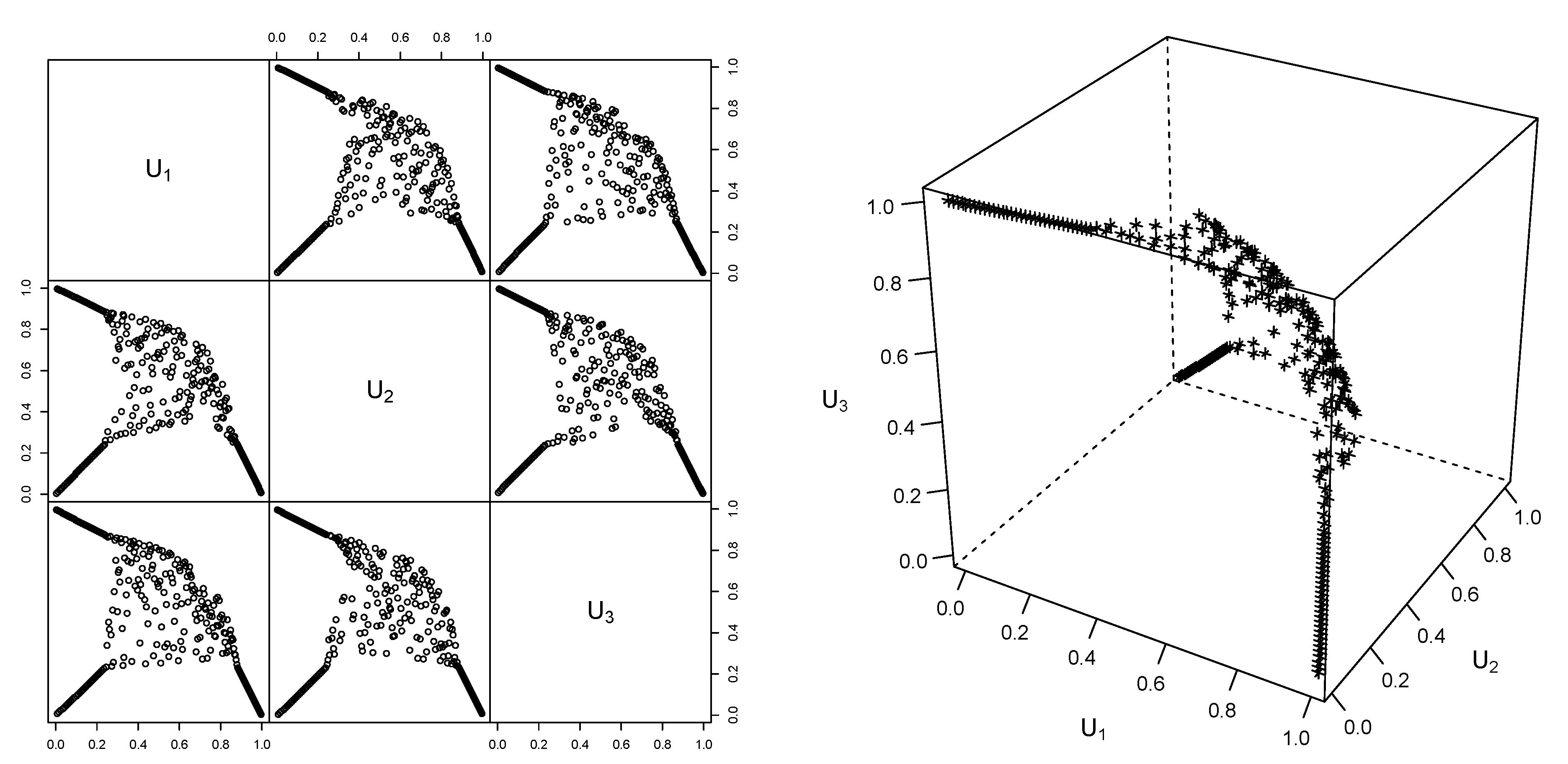
Figure 9.
Bounds and on as functions of the chosen individual relative tolerance.

© 2020 by the author. Licensee MDPI, Basel, Switzerland. This article is an open access article distributed under the terms and conditions of the Creative Commons Attribution (CC BY) license (http://creativecommons.org/licenses/by/4.0/).
Share and Cite
MDPI and ACS Style
Hofert, M. Implementing the Rearrangement Algorithm: An Example from Computational Risk Management. Risks 2020, 8, 47. https://doi.org/10.3390/risks8020047
AMA Style
Hofert M. Implementing the Rearrangement Algorithm: An Example from Computational Risk Management. Risks. 2020; 8(2):47. https://doi.org/10.3390/risks8020047
Chicago/Turabian StyleHofert, Marius. 2020. "Implementing the Rearrangement Algorithm: An Example from Computational Risk Management" Risks 8, no. 2: 47. https://doi.org/10.3390/risks8020047
Note that from the first issue of 2016, this journal uses article numbers instead of page numbers. See further details here.