Article

A Longitudinal Analysis of the Impact of Distance Driven on the Probability of Car Accidents

by
Jean-Philippe Boucher
* and
Roxane Turcotte
Département de Mathématiques, Université du Québec à Montréal (UQAM), Montréal, QC H3C 3P8, Canada
*
Author to whom correspondence should be addressed.
Risks 2020, 8(3), 91; https://doi.org/10.3390/risks8030091
Submission received: 20 July 2020 / Revised: 25 August 2020 / Accepted: 26 August 2020 / Published: 1 September 2020

Abstract

:
Using telematics data, we study the relationship between claim frequency and distance driven through different models by observing smooth functions. We used Generalized Additive Models (GAM) for a Poisson distribution, and Generalized Additive Models for Location, Scale, and Shape (GAMLSS) that we generalize for panel count data. To correctly observe the relationship between distance driven and claim frequency, we show that a Poisson distribution with fixed effects should be used because it removes residual heterogeneity that was incorrectly captured by previous models based on GAM and GAMLSS theory. We show that an approximately linear relationship between distance driven and claim frequency can be derived. We argue that this approach can be used to compute the premium surcharge for additional kilometers the insured wants to drive, or as the basis to construct Pay-as-you-drive (PAYD) insurance for self-service vehicles. All models are illustrated using data from a major Canadian insurance company.

1. Introduction

In the past decade, new technologies such as GPS-collected data have emerged, which offer new ways to approach car insurance pricing. Processing these data provides reliable information about drivers’ behavior. Before GPS and telematics devices, the insurance industry had to rely on proxy variables such as territory, gender and age of the drivers to measure risk. However, such covariates only describe the general behavior of insured in those groups. For example, Ayuso et al. (2016b) shows that the differences observed in claims frequency between men and women are largely attributable to vehicle use; Verbelen et al. (2018) reached a similar conclusion. In a social-political context where the use of gender in ratemaking is restricted or criticize, calculating premiums on more objective information is of interest.
One piece of GPS-collected information that is directly related to the risk insured is distance driven. The relevance of including this variable in ratemaking has been studied by Ayuso et al. (2014), Ayuso et al. (2016a), Boucher et al. (2013) and Lemaire et al. (2016) among others. Boucher et al. (2017) studied the effect of distance driven and policy duration time on claim frequency and challenged the usual ratemaking practice of using contract duration as the risk exposure measure. Mileage-based pricing can generate several benefits, notably on the environment, because it encourages policyholders to reduce their annual mileage. Establishing premiums on the basis of variables that the insured can control has the significant advantage of encouraging a positive change of habit in policyholders (see for example Bolderdijk et al. (2011) and Tselentis et al. (2016)). One can argue that distance driven is correlated with other driving habits resulting from driving experience, (Ferreira and Minikel (2010)). Hence, if the model does not take this correlation into account, the resulting relationship between claim frequency and the distance driven would not give an appropriate representation of how the claim frequency could change when insureds change their driving habits. This is precisely what is tackled in this paper: we indeed focus on the “marginal” effect of distance driven. The objective of our paper is not to compute a premium, but mainly to understand how the distance impacts the claim frequency when all individual characteristics of policyholders have been considered.
We focus our analysis on the distance driven, yet other telematics variables could be of interest. In the study by Verbelen et al. (2018), driving time (daytime vs. nighttime) is studied along with the type of roads, while Ma et al. (2018) find that speed and acceleration affect the expected claim frequency. Ayuso et al. (2014) analyze the effect of various covariates for the time before the first crash, and compare novice and experienced drivers. More recently, Ayuso et al. (2019) propose to improve the traditional ratemaking methods by including information related to risk exposure and driving behavior of insured. Denuit et al. (2019) use predictive rating with past telematics information in a credibility model. Weidner et al. (2016) study driving behavior and vehicle use on different scales of analysis (maneuver, trip or insurance period) by means of form recognition and Fourier analysis methods. Wüthrich (2017) proposes to use speed and acceleration heat-maps to classify drivers into groups using K-means clustering. Each group is associated within a driving style and included as a categorical variable in a regression analysis. Gao and Wüthrich (2018) performed principal component analysis using singular value decomposition and bottleneck neural networks. The authors argue that a representation in two dimensions is sufficient to preserve most of the driving information, meaning that it is possible to obtain continuous representations with small-dimensional data. This representation could then be included in a Generalized Additive Model (GAM), as in the study by Gao et al. (2019). Verbelen et al. (2018) evaluate the predictive power and interpretability of telematics variables on claim frequency by comparing various types of models that include or exclude those telematics variables. The authors find that the best ratemaking structure includes both telematics and traditional covariates, while considering duration and mileage as exposure measures.
In Section 2, we present the dataset used for the numerical applications throughout this work and we compare different exposure measures. In Section 3, we used a GAM Poisson, as did Boucher et al. (2017), to link the distance driven with the number of claims. We observe the same relationship between distance and claims frequency; however we reject the “learning effect” explanation proposed by previous authors to explain the relationship, which we posit can be explained by the residual heterogeneity incorrectly captured by the underlying GAM model. Section 4 presents panel count data models that are better suited to explain individual heterogeneity. In Section 5, using Generalized Additive Models for Location, Scale and Shape (GAMLSS, see Rigby and Stasinopoulos (2005)) theory that generalizes GAM, a multivariate count distribution for all the contracts of the same insured is developed, and a penalized log-likelihood is used to estimate the parameters. In Section 6, we use another approach based on a Poisson distribution with fixed effects to account for all individual characteristics, and show that an approximately linear relationship between the distance driven and claim frequency can be found. Section 7 concludes.

2. Summary of the Database

The dataset that has been used for our numerical analysis comes from an important Canadian P&C insurance company. We focus our analysis on personal car insurance from the province of Ontario.
In analyzing telematics data, we must be careful before jumping to general conclusions about driving behavior of the whole portfolio. Indeed, policyholders who decided to place a telematics device on their car, or to download an application on their phone that tracks all their car trips, do not correspond to the general driver population. In our case, approximately 10% to 15% of the insurance company’s portfolio chose to use the telematics option for their car insurance. Typically, these insureds correspond to one of the two following profiles:
  • Policyholders who are technophiles: they love new telematics technology, and want detailed information about their driving habits. Summary driving data is indeed continuously available to policyholders via a website.
  • Young and/or bad drivers. To motive policyholders to buy the telematics option, insurance companies often offer an initial discount, and the renewal discounts range from 0% to 25% depending on driving experience.1 Because auto insurance in Ontario is very expensive and often unaffordable for some drivers, all discounts are welcome for policyholders with high insurance premiums. As a result, an unusually high proportion of risky insureds uses telematics devices or telematics app.
In the dataset used, we observed the insureds for up to six insurance periods, with an average of 1.77 contracts per policyholder (see Table 1 for details). Only policyholders that have been observed at least 100 days were retained for the analysis. Since this is real data, it may contain some minor irregularities. The same table shows statistics for the number of claims, where we only kept claims related to road accidents. Indeed, we wanted to study accidents related to car usage and not, for example, those caused by floods, hail, theft or vandalism. The table shows statistics for a single insured period. We note that most policyholders do not claim, that the average claim frequency for the portfolio is 6.0%, and that the maximum number of claims observed is 3.

Risk Exposure Measures

Table 2 summarizes the statistics of various risk exposure definitions:
  • Exposure time (the time between the start and the end of the insurance contract)
  • Distance driven
  • Number of trips
  • Hours driven.
Another candidate for risk exposure might be the self-reported approximation of the distance driven by the insured. However, as shown by many authors, such as Lemaire et al. (2016), the self-reported distance driven is not reliable and is often very different from the exact distance driven.
Exposure time, traditionally used by insurers, would be an appropriate measure of risk exposure if every driver had about the same car usage, which is not the case. Indeed, Table 2 shows that for an insured period, insureds drove between 7.1 and 76,272 km, with an average of 10,398 km. More specifically, the database also informed us about various types of car use by the insureds:
  • The maximum number of trips observed is 3317 while another one only used his car 15 times for a single insured period.
  • A policyholder drove the car for only for one hour for the whole insured period, while another driver used the car for more than 3000 h.
Consequently, there are important differences between driving uses and driving habits, which justifies consideration of other measures than exposure time in the modeling.
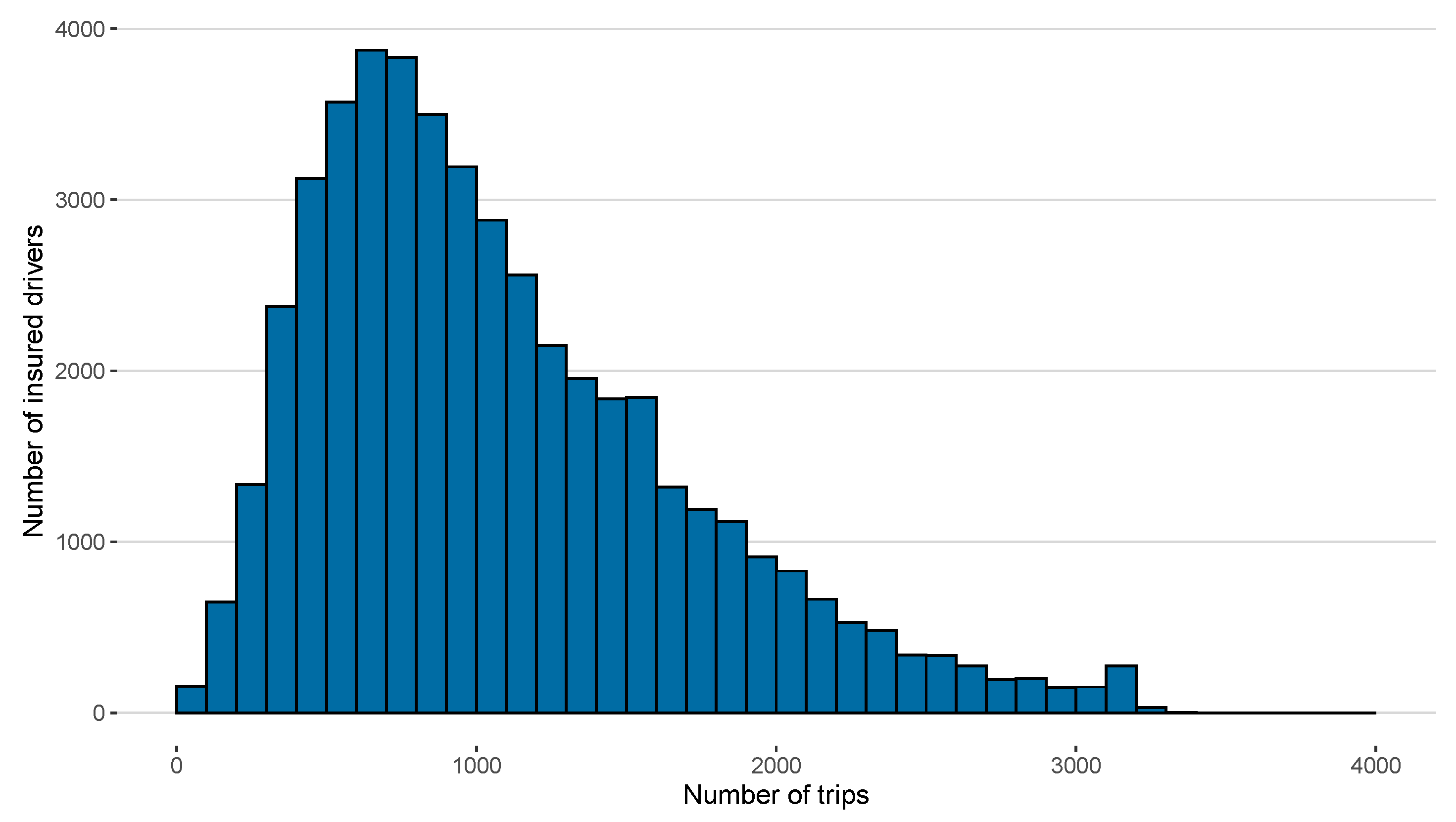
Figure 1, Figure 2, Figure 3 and Figure 4 shows histograms of different risk exposure measures under study. Except for exposure time, every other risk exposure distribution is right-skewed. Table 2 foreshadowed this result as the average was greater than the median for those risk exposures. This is another indication that some insureds make full use of their insurance time by making greater use of their car.
Figure 5, Figure 6, Figure 7 and Figure 8 illustrate the links between claim frequency and risk exposure. A fairly clear linear trend seems to be emerging for the three non-traditional exposure measures for the first part of their respective curve, which contains most of the observations. However, we observe a strange relationship between the claims frequency and the risk exposures for higher quantiles of the distributions. We specify that each point on these graphs does not represents the same number of policyholders. Darker dots represent a larger number of policyholders.
Between the three usage-based exposure measures, our choice for a more detailed analysis is distance driven. First, it seems to be the objective measure of risk of the three. Indeed, the definition of a “trip” is not clear. For example, if the driver makes a quick stop to buy gas, does it count for one or two trips because the engine stopped? For hours driven, does the time spent stopped at red lights and stuck in traffic count similarly to when the vehicle is moving? Second, it would be hard to measure exposure only according to the number of trips from a marketing point of view because those who use their vehicle only to drive short distances would probably find it unfair.

3. Preliminary Risk Exposure Analysis

Traditionally, the starting point for the modeling of the number of claims N i from a policyholder i exposed to the risk of a term t is modeled by a Poisson distribution of average t λ i , where λ i includes classic covariates used in pricing. For a Poisson regression, t is often referred to as an offset variable. Similarly, for an insured driving a car over a distance of d km, we are seeking a model with this form of proportionality between distance driven and the expected claim frequency. Also, it could be interesting to combine t and d in the same model. To do this, one avenue is to use generalized additive models (GAM).
GAMs, introduced by Hastie and Tibshirani (1986), are an extension of the generalized linear models (GLM) theory. Consequently, as for the GLM, only distributions belonging to the linear exponential family could be used as the distribution of the response variable of a GAM. In a GLM, the linear predictor for an individual i is given by g ( μ i ) = X i β , where X i = [ x 1 , i , x 2 , i , x 3 , i , ] is a vector of covariates and β is a coefficient vector. For a GLM, the mean is given by a linear expression through a link function: GAMs relax the hypothesis of linearity, and smoothing functions s of the covariates could be included in the predictor. For example, the mean for an individual i could be given by g ( μ i ) = s 0 + s 1 ( x 1 , i ) + s 2 ( x 2 , i ) + s 3 ( x 3 , i ) , where s 0 is an intercept, s k are smoothing functions and x k , i are covariates for k { 1 , 2 , 3 } .
Boucher et al. (2017), by using a GAM Poisson model, analyzed the influence of duration and distance driven on the number of claims with independent cubic splines and splines with a tensor product to introduce a dependence between those two risk exposure measures (see Green and Silverman (1993) for additional details on these smoothing functions). The model with independent cubic splines is the starting point of our analysis, and we evaluate the performance of this model on our data. The model log ( μ i ) = β 0 + s 1 ( k m i ) + s 2 ( d i ) yields similar results to those obtained by Boucher et al. (2017), as it can be seen in Figure 9. Indeed, we observe a strongly increasing function for the first kilometers, then it stabilizes around 40,000 km. For the higher quantile of the distribution, there are very few observations, and the confidence interval is too wide to draw conclusions. As for s 2 ( d i ) , we observe a positive effect for the duration time, but no linear relationship because the function tends to stabilize. For the sake of completeness, the model with a tensor product has been fitted on our data. The tensor product includes dependency between the two exposure measures, and the fitted surface had a shape similar to that of Boucher et al. (2017). Considering the important differences between the European dataset used in Boucher et al. (2017) and our North American data, the similarity of the results is fairly interesting. First, climatic conditions are not the same given the significant accumulations of snow on the ground during Canadian winters. Second, the profile of policyholders between the two databases is not the same. The Spanish data focused exclusively on young drivers while Canadian data’s profiles are more diverse as explained in Section 2. It can also be noted that the data are collected over different years for the two databases and the regulations differ from one country to another.
We investigate the smoothing functions on the scale of the response level ( exp ( s 1 ( k m ) ) and exp ( s 2 ( d ) ) ) to expose the multiplicative effect on λ i , t , as illustrated in Figure 9. Specifically, with a log link function, we have
μ i , t = exp ( X i , t β + s 1 ( k m ) + s 2 ( d ) ) = exp ( s 1 ( k m ) ) exp ( s 2 ( d ) ) exp ( X i , t β ) = exp ( s 1 ( k m ) ) exp ( s 2 ( d ) ) λ i , t ,
In the study by Boucher et al. (2017), a “learning effect” is advanced to justify the look of s ^ 1 ( k m ) (and exp ( s ^ 1 ( k m ) ) ), where the expected number of claims seems to decrease as kilometers driven increases. We think that this effect cannot be used as an explanation. Indeed, most drivers in the insurance portfolio already have many years of driving experience. We do not think that the extra 10,000–20,000 km adds enough experience to observe a learning effect.
Instead, we think that the shape of the smoothing function comes from the driver profiles: the lower quantiles of the distribution of the distance driven does not come from the same (type of) drivers as the higher quantiles. This means that models based on Figure 9 cannot be used to understand the relationship between the distance driven and the number of claims, and might not be used to set the premium for insured that suddenly change their driving habits, because it does not nearly tell us how their risk is changing.
As an example to illustrate the situation, we can suppose an insured who suddenly decides to drive 50,000 km instead of 40,000 km. Based on Figure 9, we would expect a decrease in the expected claims frequency. This is however impossible: the number of claims in the first 40,000 km cannot change, and the extra 10,000 km can only add other claims. In other words, if insureds choose to drive their cars rather than leaving it at home, the risk should always be greater. The slope could change as distance increases, but it should always be strictly positive since the risk is greater, meaning that the smoothing function (as the one observed in Figure 9) should always be increasing.
Our results, and those of Boucher et al. (2017), do not show a strictly positive relationship between claim number and distance driven. We think that this can be explained by the residual individual heterogeneity of the model, which the basic Poisson GAM does not seem to capture correctly. One explanation comes from the fact that GAM supposes independence between all contracts of the same insured. We think that a more general model that relaxes this assumption should be used to correctly measure the impact of the distance driven on the risk of accidents.

4. Panel Data Modeling

When all observations are considered independent, we usually refer to it as cross-sectional data. Basic GLM and GAM are constructed under such an assumption. In non-life insurance, however, we can observe the same insured over many contracts. Consequently, we can generalize the approach by supposing a dependence between all those contracts. This dependence is usually justified by the fact that many important factors cannot be used as covariates in ratemaking.
Formally, suppose that we observe an insured i for over T contracts. Instead of modeling the marginal distribution of each N i , t for t = 1 , , T , we are now looking for the joint distribution (subscript i is removed for convenience):
Pr ( N 1 = n 1 , N 2 = n 2 , , N T = n T ) = Pr ( N 1 = n 1 ) × Pr ( N 2 = n 2 | N 1 = n 1 ) × × Pr ( N T = n T | N 1 = n 1 , , N T 1 = n T 1 ) ,
where N t , t = 1 , , T , is the number of reported accidents for insured period t. There are many ways to construct multivariate count models (see Inouye et al. (2017) or Molenberghs and Verbeke (2006) for example). One popular way, which draws a parallel with the explanation of the unused covariates in the modeling, is to include an individual parameter α in the mean parameter of the count distribution of each contract t, which means that we have:
N i , t Poisson ( μ i , t = α i λ i , t ) ,
where λ i , t = exp ( x i , t β ) for i { 1 , , n } and t { 1 , , T i } . For an insured i, the key to the dependence then lies in the parameter α i which affects all the random variables N i , t for t = 1 , , T . We can consider two different situations regarding this parameter:
  • All α i , i = 1 , , n are i.i.d. random variables that come from a selected prior distribution (we call this the random effects model, studied in detail in Section 5);
  • All α i , i = 1 , , n are unknown parameters that need to be estimated (we call this the fixed effects model, studied in detail in Section 6).
In both cases, random and fixed effects models give us the flexibility to create a joint distribution that allows for time dependence. However, even if they share some similarities, random and fixed effects models are different, and the differences between them are highlighted when we consider telematics data and the distance driven.

5. Random Effects

5.1. Model Specification

In random effects models, we suppose that α i , i = 1 , , n , are random variables, with prior density f ( · ) . Conditionally on the random effects α i R E , all numbers of claims N i , 1 , N i , 2 , , N i , T from insured i are independent. As shown in Denuit et al. (2007), the joint distribution of N i , 1 , , N i , T can be expressed as:
Pr [ N i , 1 = n i , 1 , , N i , T = n i , T ] = 0 t = 1 T exp ( α i R E λ i , t R E ) ( α i R E λ i , t R E ) n i , t n i , t ! f ( α i R E ) d α i R E .
Many distributions can be used for α i R E , such as the gamma or the inverse Gaussian. If we suppose that α i R E follows a gamma distribution of mean 1 and variance 1 ν , the joint distribution can be expressed as:
Pr [ N i , 1 = n i , 1 , , N i , T = n i , T ] = t = 1 T ( λ i , t R E ) n i , t n i , t ! Γ ( n i , + ν ) Γ ( ν ) ν λ i , R E + ν ν λ i , R E + ν n i , ,
where n i , = t = 1 T n i , t and λ i , R E = t = 1 T λ i , t R E . This well-known distribution is the multivariate negative binomial distribution, or simply MVNB. This distribution is a generalization of the negative binomial distribution. It is a basic distribution for panel count data modeling with overdispersion ( E [ N i , t ] = λ i , t R E < V [ N i , t ] = λ i , t R E + ( λ i , t R E ) 2 / ν ).
It can be shown that the first-order condition to obtain β ^ M L E is:
i = 1 n t = 1 T x i , t n i , t λ i , t R E n i , + ν λ i , R E + ν = 0 .
This model is based on a distribution which is not a member of the linear exponential family. That means that GAM theory cannot be used to include smoothing functions. Instead, we use Generalized Additive Models for Location, Scale and Shape (GAMLSS) (see Rigby and Stasinopoulos (2005)) theory, that can be used for other distributions than the members of the linear exponential family of distribution. Moreover, a GAMLSS is more flexible because it can model a location parameter μ i , a variance parameter σ i (scale), a skewness parameter ν i and a kurtosis parameter τ i as additive functions of the covariates. The general form is given by
g k ( θ k ) = X k β k + j = 1 J k Z j , k γ j , k
where θ = { μ , σ , ν , τ } . μ , σ , ν and τ are vectors with n elements. For each g k ( θ k ) , it is possible to add the desired number J k of additive terms. These terms could be, for example, smoothing functions or random effects.
A model does not need to specify each of the components of θ . For example, it is possible to use a GAMLSS that specify only the location parameter. In this case, θ would simply become θ = { μ } . For our telematics data, we choose to model the parameter λ i , t with smoothing function by Equation (5), and ν is kept constant for all individuals.
Please note that in Equation (5), X k β k represents the parametric part that is present in GLMs and j = 1 J k z j , k γ j , k is the non-parametric part. X k is a known design matrix of dimensions n × J k and β k is a vector of parameters of length J k , which corresponds to the number of covariates in the parametric part of the model. As for z k and γ k , they are respectively a known design matrix of dimensions n × q j , k and a vector of random variables of length q j , k . The shapes of z k and γ k depend on the additive functions used. If a smooth function can be expressed in linear form, Equation (5) can be rewritten as
g k ( θ k ) = X k β k + j = 1 J k h j , k ( x j , k ) ,
where h j , k is a smooth non-parametric function.

5.2. Numerical Illustration

To use GAMLSS, many distributions are available in the R package gamlss. Unfortunately, the MVNB distribution is not one of them (the distribution is however implemented by itself in the package multinbmod). Consequently, we have to write our own code for convenience. As shown in Equation (6), to fit the model, we maximize a penalized log-likelihood function l p , integrating a quadratic penalty γ T G γ , where G is a penalty matrix for the vector of random effects parameters γ . The penalty matrix G is very often define as Λ D r T D r , where different formulations are possible for D r . In our work, D r is a ( q j , k r ) × q j , k difference matrix of order r as defined in Rigby and Stasinopoulos (2005), taking r = 2 (default). r corresponds to the argument “order” in R function pb.control for P-splines. A hyper-parameter, noted here Λ R + , controls the weight given to the penalty and, thus, the smoothness of the smoothing function. The greater its value, the smoother the resulting estimated function. K = 2 penalties are added in the log-likelihood, one for each smoothing function included in the model. l stands for the log-likelihood of the joint distribution associated with Equation (3).
l p = l 0.5 k = 1 2 j = 1 J k γ j , k T G ( Λ ) j , k γ j , k
The model is constructed as follows. As in Section 3, the mean parameter is represented by (1). On the other hand, unlike Section 3, we now work with cubic P-splines as our smoothing functions. Choosing the optimal number of nodes in a regression spline is not an obvious task. In Section 3, the number of nodes was determined by trial and error with different combinations for the two smooth functions. The number of nodes was chosen graphically using the representation of the smoothing function (Figure 9) to compromise between the accuracy of the data and smoothness. We now try a different approach that does not require us to select several nodes.
In a P-spline, we choose a relatively large number of knots, and wiggliness is controlled by a penalty parameter for each smoothing function. For instance, we used 20 knots for each spline, but “a relatively large number of knots” depends on your context and data. P-splines are smoothers based on B-splines with a difference penalty on coefficients of adjacent B-splines, which are strictly local polynomial functions (of a degree three, for our use). For further information on B-splines and P-splines, refer to Eilers and Marx (1996) and Wood (2017). P-splines have the advantage of offering flexibility without being cumbersome to implement.
To select the penalty parameters in G ( Λ ) associated with both p-splines of the contract duration and the distance traveled, we test out multiple combinations of values of Λ = { Λ 1 , Λ 2 } . We proceed in two steps: we first adjust the model for all the couples of a grid of parameters. Large steps are used to cover an interval ranging from small values to very large values for Λ 1 and Λ 2 . Then, we examine the regions in which the parameter value models with the best AIC are obtained, and we restart a more specific search in these regions with smaller steps. Following multiple estimations of models, the best model was selected based on the AIC criteria that consider the number of effective degrees of freedom and the interpretability of the results.
Please note that this model was also fitted with a few covariates: gender (female or other), marital status (married or other) and vehicle usage (commute, pleasure or other). As shown in Equation (1), covariates can be added in the λ i , t parameter. Adding covariates does not change the shape of the splines, but it does tend to increase the value of ν as more heterogeneity is explained.
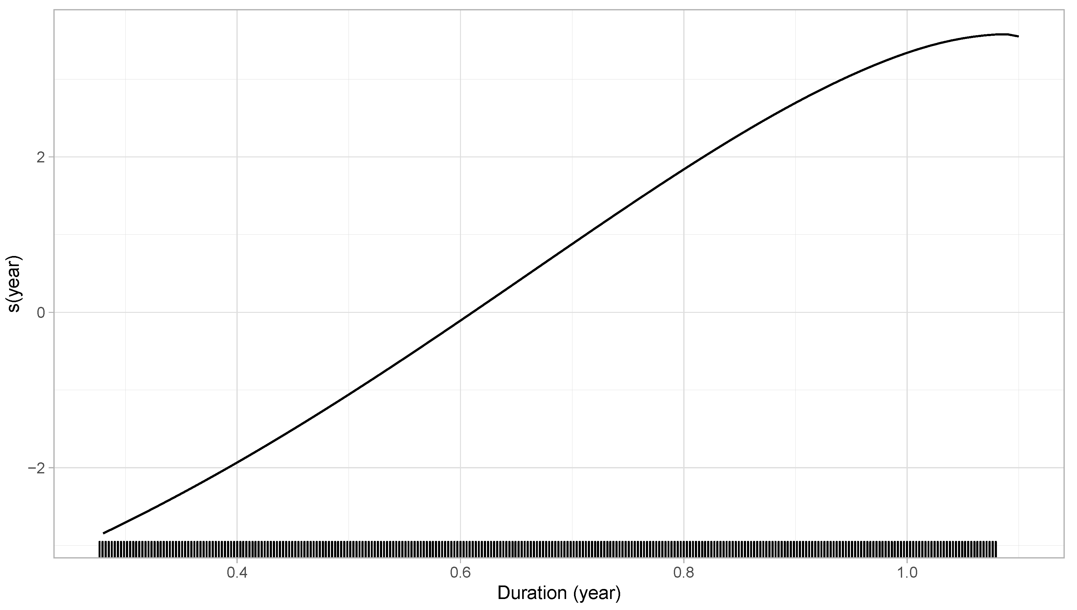
The fitted smooth functions are illustrated at Figure 10. We can see that the functions are very different from Figure 9. Indeed, even if we observed a similar decrease for the upper quantile of the distribution for the distance traveled, the highest point before the decrease is at a later point where the data are very scarce. This can be seen as an improvement over the previous model: we obtain a strictly positive relationship between claim number and distance driven until 60,000 km driven. For the contract duration, Figure 11 shows a nearly proportional relationship between the time exposure and the claims frequency, hence similarities with Figure 9.
As mentioned, the MVNB distribution is not available in the gamlss package and the confidence bands displayed in Figure 10 were generated by bootstrap. We turn to this alternative, because the penalty in P-splines does not allow calculating confidence intervals as easily as in the case of B-splines. Bootstrap is a common approach to deal with this problem. We resampled with replacement a sample of size n. Given the estimated parameters from the maximum penalized log-likelihood procedure, except for the parameters of the spline for which we wish to construct the confidence bands, we estimate the parameters of the spline with this re-sample. We repeat these steps many times to construct an empirical distribution for each parameter of the spline. We construct the lower (upper) band of the spline by taking the 5th (95th) percentile of each parameter distribution. Each repetition of this procedure could take some computational time, but it converges with a relatively small number of iterations. As is usually recommended, we used 1000 repetitions to find those values. We found that the values of the 5th and 95th percentile of a 100-repetition-bootstrap are very similar to the percentiles of a 1000-repetitions-bootstrap. Considering the calculation time required for this procedure, this is an advantage that the bootstrap stabilizes quickly.
To conclude the MVNB, note that this distribution and other panel distribution for claim counts can be used for predictive rating, where it can be shown that the predictive distribution of N i , T depends on past values of λ i , t and n i , t , for t = 1 , , T 1 . To illustrate the situation, we obtained a value of ν ^ = 6.57 for an MVNB with contract duration as an offset, but without driven distance, while the final GAMLSS model with 2 splines based on the MVNB generates ν ^ = 8.25 . Without going into details, given that our objective for this paper is to measure the impact of distance driven, it means that a rating structure based on MVNB with telematics information reduces the unexplained variance of the model, while offering smaller penalties/discounts for drivers who claim/do not claim. We refer to Denuit et al. (2019) for predictive rating models with telematics information.

6. Fixed Effects

6.1. Model Specification

In the fixed effects model, we consider each α i , i { 1 , , n } as an unknown parameter. One approach would then be to estimate all those parameters, as well as the p parameters associated with the covariates, by maximum likelihood. That means that at least n + p + 1 parameters should be estimated, which is quite a high number of parameters given that T i is usually small for insurance datasets. The problem with this ML estimation is that it does not necessarily generate convergent estimates in the classical case of a T fixed and n . Moreover, the large number of parameters in the model causes what is called incidental problem, which means that an incorrect estimation of the fixed effects α generates incorrect estimates of β associated with covariates in the mean. In the case of a logistic regression, for example, it has been shown that the β ^ M L E were indeed biased. However, hopefully, it has been shown that a fixed effects model based on a Poisson distribution does not have this problem (see Cameron and Trivedi (2013) for a detailed explanation).
Consequently, for a fixed-effect Poisson regression model of mean α i F E λ i , t F E , it can be shown that the first-order condition to obtain each α i is simply
α ^ i = n i , λ i , ,
where α i for each insured i was directly estimated using MLE. For the β parameters, the first condition by MLE can be shown to be equal to:
i = 1 n t = 1 T i x i , t n i , t λ i , t F E n i , λ i , F E = 0 .
When looking closely at this equation, some details about β estimation for fixed effects can be deduced.
(1)
When we compare Equations (4) (first-order condition equation of the random effects model) and (8), we see that when T is large, or when ν 0 , random and fixed effects models are equivalent. However, in our data, the number of contracts T i observed for each insured i is small, while ν ^ is significantly greater than zero. This results in different estimation equations between the two models.
(2)
Individuals observed for a single insured period, i.e., with T i = 1 , are not considered in the estimation of the β parameters;
(3)
Individuals who have not filed claims with the insurer do not contribute to the estimation either. Indeed, for an individual i that does not have a claim, we have t = 1 T x i , t 0 λ i , t F E t × 0 λ i , F E = 0 which is constant, whatever the value of β .
(4)
It is necessary to restrict the covariates x i , t included in λ i , t F E to those that change over time. Consequently, this also rules out the inclusion of an intercept in the model.
(5)
If λ i , t F E does not change over t = 1 , , T i for an individual i, this policyholder does not contribute to the estimation (even if they claimed). The ratio λ i , t F E λ i , F E is the key element in the estimation of β , where it is used to find the best “weight” to apply at each n i , t to approximate n i , . In other words, to measure the specific effect of a covariate x , the driving experience of an insured must be measured with and without the effect of x . For the distance driven, this seems to be exactly what we are looking for. Indeed, as mentioned in Section 3, we are looking for the marginal impact of each extra kilometer driven when insureds decide to use their car rather than leaving it at home.

6.2. Poisson Fixed Effects and Smoothing Functions

We show that fixed effects modeling with smoothing functions is possible using the GAM theory. Indeed, as mentioned Cameron and Trivedi (2013), each α i can be seen as a simple covariate identifying the insured i. Consequently, by
  • removing insureds without claim,
  • removing insured observed for only one insured period T i ,
  • adding a factor covariate x for insured identification,
the Poisson fixed effects model can be seen as a basic Poisson regression model without an intercept. Being part of the linear exponential family of distribution, GAM theory can then be used when smoothing functions are added to the mean parameter of the distribution.

6.3. Numerical Illustration

In practice, as mentioned, it is relatively easy to implement the fixed effects model with R; we simply used the gam function from the package mgcv. To include fixed effects in the model the intercept of the model is dropped. We include a unique identifier variable for each policyholder as a factor variable and we include the distance driven in the model using a cubic spline s. As for the GAM of Section 3, we used a cubic spline for the modeling. The cubic spline yields to very similar results to those for a penalized spline, but for a fraction of the computation time. Unlike the two previous approaches, we decided to illustrate the usage of the Poisson fixed effects by not including a smoothing function for the duration because our objective in this research is to measure the marginal effect of the distance on the claim frequency. If we want to measure the risk of each additional kilometer the insured decides to drive, the duration of the contract is not important. Put another way, we want to construct a rating structure based solely on the distance driven as a risk measure. Figure 12 shows the results for the relationship between exp ( s ( k m ) ) and claim frequency.
For the fixed effects model, we see that the relationship between the distance traveled on the claim frequency is always increasing, and is even almost linear. To highlight this linear effect, a line had been added to the graph to show how close the relationship is to a linear relationship. Toward the end, there is a noticeable deviation from the linear relationship, but only 0.3% of the observations are beyond this point, which is not very significant. What has been called the “learning effect”, observed in Section 3, has disappeared and we observe a much more logical and coherent relationship between distance traveled and frequency than before. The relationship between claim frequency and the distance driven should be understood as the marginal impact of each additional kilometer driven or not-driven. Explicitly, as we approximated exp ( s ( k m ) ) by 0.25 + 1 15,000 k m i , t (the red line in Figure 12), we then have
N i t P o i s s o n exp ( α i ) exp ( s ( k m ) ) P o i s s o n exp ( α i ) ( a + b k m i , t ) P o i s s o n 0.25 exp ( α i ) + 1 15,000 exp ( α i ) k m i , t .
We see that the slope, i.e., the marginal impact of each additional kilometer driven or not-driven, is not the same for each insured because it depends on α i . To illustrate this difference, we use the estimated values of α i for several insureds. Figure 13 shows the relationship between claim frequency and distance driven for different individuals (the policyholder with the minimum, maximum, median, 25th and 75th percentile individual parameter value). With this model, we then reconcile the intuition that each kilometer should increase the risk for an individual, but that this increase could be different for each driver.
In summary, instead of referring to the “learning effect” to understand the left-hand graph of Figure 9, we should understand instead that typical insureds who drive more than 60,000 km per year are better risks per kilometer than insureds who drive approximately 40,000 km per year. That obviously does not mean that insureds that drive 40,000 km per year should drive 60,000 km to reduce their risk. The difference between insureds related to their risk per kilometer can be explained by many factors: more frequent use of the highway, higher proportion of driving outside rush hours, etc. However, for each driver, independently of their driving risk per kilometer, the risk of an accident will always increase for each additional kilometer driven (by approximately 1 15,000 ).
To conclude about the fixed effects model, note that the risk is still present even when the driving distance is zero. This is counter-intuitive because we can presume that someone who does not drive at all should have an expected claim frequency of zero. We agree. However, the real risk exposure is never completely null and the intercept could represent situations where an accident is possible even without driving a lot (e.g., it may occur very close to the insured’s home). Moreover, even if the car would never actually be used, hit and run situations are also possible.

6.4. Which Effect Should Be Used in Practice?

Random and fixed effects seem to generate contradictory results, and we may wonder which model we should then use in practice, particularly for ratemaking. This has already been discussed in the actuarial literature by Boucher and Denuit (2006), but it is worth reexamining it in the context of telematics data, for distance driven in our case.
First, the fixed effects model is more general than the random effects model, which means that in case of contradictory results, fixed effects should always be preferred. Equation (3) can be derived as:
Pr [ N i , 1 = n i , 1 , , N i , T = n i , T ] = 0 Pr [ N i , 1 = n i , 1 , , N i , T = n i , T | x i , 1 , , x i , T , α i R E ] f ( α i R E | x i , 1 , , x i , T ) d α i R E = 0 t = 1 T Pr [ N i , t = n i , t | x i , 1 , , x i , T , α i R E ] f ( α i R E ) d α i R E = 0 t = 1 T exp ( α i R E λ i , t R E ) ( α i R E λ i , t R E ) n i , t n i , t ! f ( α i R E ) d α i R E
We can see that we have to suppose an additional assumption: from the first to the second line of development, f ( α i R E | x i , 1 , , x i , T ) becomes f ( α i R E ) . That means that we must suppose that random effects are independent of observed covariates. Empirical analyses have shown that this is not the case. Indeed, as shown by Boucher and Denuit (2006), random effects do not have the same distribution for young drivers as for older ones, and depends on gender, for example. However, this is a typical assumption made in actuarial science, and Boucher and Denuit (2006) discusses the consequences of not satisfying this assumption. The authors concluded that the interpretation of random effects results are tricky.
On the other hand, fixed effects modeling, even if theoretically better, is not amenable to ratemaking:
  • The model requires evaluating an individual parameter α i for each insured i in the portfolio. This raises a problem for new policyholders.
  • For a small value of T i , α ^ i may be incorrectly estimated.
  • As the model estimates each individual α i as n i , λ i , , policyholders without claims will have an expected number of claims of 0, meaning that the premium of these insureds should be zero.
As Boucher and Denuit (2006) conclude for basic ratemaking purposes, even if theoretically problematic, the random effects model should be preferred over a fixed effects model: random effects are flexible enough to compute premiums for new insureds, and do not generate a premium of 0 for insureds without claims. However, actuaries must understand that the parameters obtained by random effects models only indicate the apparent effect of the covariates, and not a causal effect (or what might be call the real impact).
To compare the fixed effects results with those of the random effects model, the approximate relationship for the median value of the individual parameter α ^ i has been plotted over the smoothed function of distance traveled of the random effect approach (see Figure 14). Interestingly, the two curves are similar.
Regarding the use of the results of a fixed effects model, fixed effects should be used to understand the “true” relationship between covariates and claims experience. For ratemaking, fixed effects should be used to compute the premium surcharge for each additional kilometer the insureds drive. In our case, it represents an increase of α ^ i 1 15,000 per km, for claim frequency. Using this approach, insurers will avoid the situation where an insured could see a premium reduction if, for example, he decides to drive 50,000 km instead of 40,000 km, as we saw with a basic GAM approach. Fixed effects can be used to construct PAYD insurance solely based on kilometers driven for self-service vehicles, where drivers’ profile cannot be directly used for ratemaking. Research is required in this area.

7. Conclusions

We have studied the relationship between claim frequency and the distance driven through different models by observing smooth functions. We first reproduced with our data the model proposed by Boucher et al. (2017) and observed what the authors called the “learning effect,” where the expected number of claims seems to decrease as kilometers driven increase. Given that most drivers in the insurance portfolio already has many years of driving experience, we rejected the conclusion that an additional 10,000–20,000 km adds enough experience to observe a learning effect. Instead, we supposed that the residual heterogeneity was incorrectly captured by the underlying GAM model.
We then evaluated panel data models with fixed and random effects. Using GAMLSS theory, which generalizes GAM, a multivariate count distribution for all the contracts of the same insured was developed. Smoothing functions were added in the mean parameter of the multivariate distribution, and a penalized log-likelihood was used to estimate the parameters. A grid of penalties, generating more than 1000 MVNB, was used to find the best distribution. However, again, the fitted smoothed function for the distance driven by the Poisson distribution with random effects did not seem to correctly describe the relationship between distance and claim frequency. Indeed, the expected number of claims still decreases disproportionately with kilometers driven.
We then used the Poisson with fixed effects to account for all individual characteristics. Because Poisson with fixed effects can be estimated by using covariates that identify each insured, we show that a simple GAM model without intercept can be used to include a smoothed function in the mean parameter. We then observed an approximately linear relationship between the distance driven and claim frequency when all individual characteristics have been accounted for in an individual parameter. This unravels the potential for the distance traveled as an exposure variable, even though this variable could not serve as a rating model. However, we think that the model proposed can be used to compute the premium surcharge for additional kilometers the insured wants to drive, or as the basis to construct PAYD insurance for self-service vehicle.
The new telematics data available in automobile insurance offers several new challenges. These data increase the possibility of identifying factors that make accidents more probable. Models like the fixed effects models proposed in the paper, make it possible to better capture the real effect of a covariate on risk. By using various models that do more than predict or calculate the insurance premium, research by insurers could shed light on risk in auto insurance. We therefore believe that many statistics compiled by telematics devices could be studied from such an angle in the future.

Author Contributions

The authors worked together on all aspects of the work. All authors have read and agreed to the published version of the manuscript.

Funding

Jean-Philippe Boucher and Roxane Turcotte gratefully acknowledge the financial support of Cooperators General Insurance Company through the Co-operators Chair in Actuarial Risk Analysis. The authors would also like to thank the financial support from the Natural Sciences and Engineering Research Council of Canada.

Acknowledgments

Jean-Philippe Boucher and Roxane Turcotte thank Gabriel Alepin for his help in the code of the GAMLSS model.

Conflicts of Interest

The authors declare no conflict of interest. The funders had no role in the design of the study; in the collection, analyses, or interpretation of data; in the writing of the manuscript, or in the decision to publish the results.

References

  1. Ayuso, Mercedes, Montserrat Guillén, and Ana María Pérez-Marín. 2014. Time and distance to first accident and driving patterns of young drivers with pay-as-you-drive insurance. Accident Analysis & Prevention 73: 125–31. [Google Scholar]
  2. Ayuso, Mercedes, Montserrat Guillen, and Ana María Pérez Marín. 2016a. Using gps data to analyse the distance travelled to the first accident at fault in pay-as-you-drive insurance. Transportation Research Part C: Emerging Technologies 68: 160–67. [Google Scholar] [CrossRef]
  3. Ayuso, Mercedes, Montserrat Guillen, and Ana María Pérez-Marín. 2016b. Telematics and gender discrimination: Some usage-based evidence on whether men’s risk of accidents differs from women’s. Risks 4: 10. [Google Scholar] [CrossRef] [Green Version]
  4. Ayuso, Mercedes, Montserrat Guillen, and Jens Perch Nielsen. 2019. Improving automobile insurance ratemaking using telematics: Incorporating mileage and driver behaviour data. Transportation 46: 735–52. [Google Scholar] [CrossRef] [Green Version]
  5. Bolderdijk, Jan Willem, Jasper Knockaert, E. M. Steg, and Erik T. Verhoef. 2011. Effects of pay-as-you-drive vehicle insurance on young drivers’ speed choice: Results of a dutch field experiment. Accident Analysis & Prevention 43: 1181–86. [Google Scholar]
  6. Boucher, Jean-Philippe, and Michel Denuit. 2006. Fixed versus random effects in poisson regression models for claim counts: A case study with motor insurance. ASTIN Bulletin: The Journal of the IAA 36: 285–301. [Google Scholar] [CrossRef] [Green Version]
  7. Boucher, Jean-Philippe, Ana Maria Pérez-Marín, and Miguel Santolino. 2013. Pay-as-you-drive insurance: The effect of the kilometers on the risk of accident. In Anales del Instituto de Actuarios Españoles. 19 vols. Madrid: Instituto de Actuarios Españoles, pp. 135–54. [Google Scholar]
  8. Boucher, Jean-Philippe, Steven Côté, and Montserrat Guillen. 2017. Exposure as duration and distance in telematics motor insurance using generalized additive models. Risks 5: 54. [Google Scholar] [CrossRef] [Green Version]
  9. Cameron, A. Colin, and Pravin K. Trivedi. 2013. Regression Analysis of Count Data. 53 vols. Cambridge: Cambridge University Press. [Google Scholar]
  10. Denuit, Michel, Montserrat Guillen, and Julien Trufin. 2019. Multivariate credibility modelling for usage-based motor insurance pricing with behavioural data. Annals of Actuarial Science 13: 378–99. [Google Scholar] [CrossRef] [Green Version]
  11. Denuit, Michel, Xavier Maréchal, Sandra Pitrebois, and Jean-François Walhin. 2007. Actuarial Modelling of Claim Counts: Risk Classification, Credibility and Bonus-Malus Systems. Hoboken: John Wiley & Sons. [Google Scholar]
  12. Eilers, Paul H. C., and Brian D. Marx. 1996. Flexible smoothing with b-splines and penalties. Statistical Science 11: 89–102. [Google Scholar] [CrossRef]
  13. Ferreira, Joseph, and Eric Minikel. 2010. Pay-as-You-Drive Auto Insurance in Massachusetts: A Risk Assessment and Report on Consumer, Industry and Environmental Benefits. Boston: Conservation Law Foundation. [Google Scholar]
  14. Gao, Guangyuan, and Mario V. Wüthrich. 2018. Feature extraction from telematics car driving heatmaps. European Actuarial Journal 8: 383–406. [Google Scholar] [CrossRef]
  15. Gao, Guangyuan, Shengwang Meng, and Mario V. Wüthrich. 2019. Claims frequency modeling using telematics car driving data. Scandinavian Actuarial Journal 2019: 143–62. [Google Scholar] [CrossRef]
  16. Green, Peter J., and Bernard W. Silverman. 1993. Nonparametric Regression and Generalized Linear Models: A Roughness Penalty Approach. Boca Raton: Chapman and Hall/CRC. [Google Scholar]
  17. Hastie, Trevor, and Robert Tibshirani. 1986. Generalized additive models. Statistical Science 1: 297–310. [Google Scholar] [CrossRef]
  18. Inouye, David I., Eunho Yang, Genevera I. Allen, and Pradeep Ravikumar. 2017. A review of multivariate distributions for count data derived from the poisson distribution. Wiley Interdisciplinary Reviews: Computational Statistics 9: e1398. [Google Scholar] [CrossRef] [PubMed] [Green Version]
  19. Lemaire, Jean, Sojung Carol Park, and Kili C. Wang. 2016. The use of annual mileage as a rating variable. ASTIN Bulletin 46: 39–69. [Google Scholar] [CrossRef] [Green Version]
  20. Ma, Yu-Luen, Xiaoyu Zhu, Xianbiao Hu, and Yi-Chang Chiu. 2018. The use of context-sensitive insurance telematics data in auto insurance rate making. Transportation Research Part A: Policy and Practice 113: 243–58. [Google Scholar] [CrossRef]
  21. Molenberghs, Geert, and Geert Verbeke. 2006. Models for Discrete Longitudinal Data. Berlin: Springer Science & Business Media. [Google Scholar]
  22. Rigby, Robert A., and D. Mikis Stasinopoulos. 2005. Generalized additive models for location, scale and shape. Journal of the Royal Statistical Society: Series C (Applied Statistics) 54: 507–54. [Google Scholar] [CrossRef] [Green Version]
  23. Tselentis, Dimitrios I., George Yannis, and Eleni I. Vlahogianni. 2016. Innovative insurance schemes: Pay as/how you drive. Transportation Research Procedia 14: 362–71. [Google Scholar] [CrossRef] [Green Version]
  24. Verbelen, Roel, Katrien Antonio, and Gerda Claeskens. 2018. Unravelling the predictive power of telematics data in car insurance pricing. Journal of the Royal Statistical Society: Series C (Applied Statistics) 67: 1275–304. [Google Scholar] [CrossRef] [Green Version]
  25. Weidner, Wiltrud, Fabian W. G. Transchel, and Robert Weidner. 2016. Classification of scale-sensitive telematic observables for riskindividual pricing. European Actuarial Journal 6: 3–24. [Google Scholar] [CrossRef]
  26. Wood, Simon N. 2017. Generalized Additive Models: An Introduction with R. Boca Raton: Chapman and Hall/CRC. [Google Scholar]
  27. Wüthrich, Mario V. 2017. Covariate selection from telematics car driving data. European Actuarial Journal 7: 89–108. [Google Scholar] [CrossRef]
1
Please note that it is not legally possible for an Ontario insurance company to increase the insurance premium based on the telematics information collected.
Figure 1. Histogram of risk exposure (in years) Each band has a length of 0.02 year.
Risks 08 00091 g001
Figure 2. Histogram of distance driven (in km) Each band has a length of 500 km.
Risks 08 00091 g002
Figure 3. Histogram of the number of trips Each band has a length of 100 trips.
Risks 08 00091 g003
Figure 4. Histogram of hours driven Each band has a length of 2000 h.
Risks 08 00091 g004
Figure 5. Claims Frequency vs. Exposure Time.
Risks 08 00091 g005
Figure 6. Claims Frequency vs. Distance Driven.
Risks 08 00091 g006
Figure 7. Claims Frequency vs. Number of trips.
Risks 08 00091 g007
Figure 8. Claims Frequency vs. Hours Driven.
Risks 08 00091 g008
Figure 9. exp ( s ^ 1 ( k m ) ) and exp ( s ^ 2 ( y e a r ) ) from the Poisson GAM estimated with Canadian data.
Risks 08 00091 g009
Figure 10. exp ( s ^ 1 ( k m ) ) and exp ( s ^ 2 ( y e a r ) ) from the GAMLSS with random effects model estimated with Canadian data.
Risks 08 00091 g010
Figure 11. s ^ 2 ( y e a r ) from the GAMLSS with random effects model estimated with Canadian data.
Risks 08 00091 g011
Figure 12. GAM with fixed effects estimated with Canadian data.
Risks 08 00091 g012
Figure 13. Exposure measure for different individual parameters.
Risks 08 00091 g013
Figure 14. Comparison between the random effect approach and the fixed-effect approach for the median value of the individual parameter.
Risks 08 00091 g014
Table 1. Distribution of the number of insurance periods for the database.
Number of Insurance Periods123456
Number of policyholders12,5629746342084441511
Proportion (%)46.536.112.73.11.50.0
Table 2. Descriptive statistics for a single insured period.
AverageVarianceMin.Max.25th pct50th pct75th pct
Exp. Time (in years)0.6450.0600.2771.0790.4630.5400.912
Dist. Driven (in km)10,39855,138,3767.176,2725026856113,836
Nb. of Trips1083383,1651533176219461434
Time Driven (in hours)38034,74012159248356483
Nb. of claims0.0600.0610.0003000