
Using the Unity Game Engine to Develop a 3D Simulated Ecological System Based on a Predator–Prey Model Extended by Gene Evolution


1
Department of Information Systems, ELTE Eötvös Loránd University, 1117 Budapest, Hungary
2
Department of Informatics, J. Selye University, 945 01 Komárno, Slovakia
*
Author to whom correspondence should be addressed.
Informatics 2022, 9(1), 9; https://doi.org/10.3390/informatics9010009
Submission received: 16 December 2021
/
Revised: 10 January 2022
/
Accepted: 16 January 2022
/
Published: 26 January 2022
Abstract
:In this paper, we present a novel implementation of an ecosystem simulation. In our previous work, we implemented a 3D environment based on a predator–prey model, but we found that in most cases, regardless of the choice of starting parameters, the simulation quickly led to extinctions. We wanted to achieve system stabilization, long-term operation, and better simulation of reality by incorporating genetic evolution. Therefore we applied the predator–prey model with an evolutional approach. Using the Unity game engine we created and managed a closed 3D ecosystem environment defined by an artificial or real uploaded map. We present some demonstrative runs while gathering data, observing interesting events (such as extinction, sustainability, and behavior of swarms), and analyzing possible effects on the initial parameters of the system. We found that incorporating genetic evolution into the simulation slightly stabilized the system, thus reducing the likelihood of extinction of different types of objects. The simulation of ecosystems and the analysis of the data generated during the simulations can also be a starting point for further research, especially in relation to sustainability. Our system is publicly available, so anyone can customize and upload their own parameters, maps, objects, and biological species, as well as inheritance and behavioral habits, so they can test their own hypotheses from the data generated during its operation. The goal of this article was not to create and validate a model but to create an IT tool for evolutionary researchers who want to test their own models and to present them, for example, as animated conference presentations. The use of 3D simulation is primarily useful for educational purposes, such as to engage students and to increase their interest in biology. Students can learn in a playful way while observing in the graphical scenery how the ecosystem behaves, how natural selection helps the adaptability and survival of species, and what effects overpopulation and competition can have.
1. Introduction
Computer-generated ecosystems are becoming more and more popular in informatics. Through graphical observation, a real-time 3D environment simulation can help in the monitoring of numerous events and creatures to see and understand their reactions. It can show how animals live, such as when they eat or drink, as well as how they behave toward other species, such as when they hunt or flee from predators, when they group up as a pack and explore the terrain together, or when they find a mate and reproduce. Seeing models of the simulated creatures rather than just reading the simple resulting statistical values of the populations is a more visually appealing experience that may demonstrate the animals’ habits and may aid in understanding the relationship between the animals’ attribute values and their behaviors.
In an ever-changing ecosystem, reaching a balanced equilibrium state is the most difficult goal. The population of a species fluctuates, and without stabilization, any population can become extinct in a blink of an eye. To survive in a complex ecosystem environment, animals must adapt to a variety of effects. With a simplified predator–prey model, animals in the same species are always identical; they act (behave) similarly, have the same attributes (traits), and are often indistinguishable from each other. These kinds of models are irreconcilable with real-life ecosystems, where species are under the constant development of enhancing their abilities. For example, predators evolve while sharpening their senses for hunting and prey adapts and boosts its survival skills.
All living organisms have inherited anatomy, physiological features, such as eye color, muscle and bone structure, and behavior patterns, which contain inherited traits and learned characteristics. Inherited traits are inborn, unlearned inclinations, which are genetically determined, such as survival instincts and reproduction motivations. These traits are supplemented with learned elements, which are acquired by choice or through experiences—for example, dislikes of certain foods. The combinations of these complex patterns result in even more complicated responses from each individual for every situation.
Parents genetically pass on their traits to their offspring; their genotypic combination results in the formation of unique, distinct offspring. Each individual is different from others because their genetic codes are somewhat mixed in the reproduction process. In the case of dioecious reproduction, the offspring inherit half of their genes from each parent. This is why children often look similar to their parents, but they do not look exactly like them—some of the genes that are passed on to children stay hidden. Additionally, during the process, an unexpected change (error) can occur in the DNA sequence, when the DNA is copied, due to many factors. This alteration in the genome of an organism is called a mutation. Mutational effects can be beneficial, harmful, or neutral, depending on their context or location.
In this paper, we created and implemented an evolution model and incorporated it into the simulation framework that we developed in our previous work [1], which was based on a simple predator–prey model. Our objective was to give the animals higher chances of adapting to different effects with evolutional changes. In the simulation environment model, these effects can be terrain conditions (mountains and water obstacles), other types of animal species (multiple prey and predator species), and population sizes. In Section 2, we summarize the related biological work and implementations of simulations. In Section 3, we will briefly present our previous system and detail why it was necessary to develop a new model (based on genetic selection) for stabilization. In Section 4, we present how we enhanced the predator–prey model with evolutional approaches and in Section 5, we show the steps of the implementation. In Section 6, we show and analyze some demonstration runs from the simulation program. In Section 7, we discuss potential areas of use, and in Section 8, we propose improvements to future evolutional models.
2. Related Work
The predator–prey model of Alfred J. Lotka (1925) [2] and Vito Volterra (1926) [3], which is known as “The Lotka–Volterra equations”, is one of the earliest and most well-known ecological models. This simple model has been renewed with additional and alternative ideas, such as multi-species systems and ratio-dependent functions. The early model (logistic theory and ratio-dependent functional responses) can be examined in the “The origins and evolution of predator–prey theory”, an article by Berryman [4]. In addition to predator–prey models, a similar host–parasitoid system was created by Nicholson and Bailey. Both models use differential equations to describe population growth, but neither model assumes that the growth of the victim population is affected by density dependence. A very good summary can be read in [5] by Abrams, which is about the two systems in prey evolution, coevolution and stability.
Instead of examining real-life evolution, scientists tried to create different mathematical models to calculate and determine populations with genetic tools. One of the most commonly used indicators is the “effective population size” developed by Wright [6,7], which means the number of individuals in an ideal population that take part in the reproducing process. The simplest model which uses this indicator is where all the individuals are of the same sex and selfing is permitted [8], but many other indicators exist with more complex models and formulas. However, as it is difficult to account for all important aspects in a reproducing process [9], these projected effective population numbers tend to underestimate the realized effective population size. To solve the complexity of these assets, breeding cycle formulas have been created [10] where subpopulations have the same size and generations are not overlapping. Many software products have been developed to simulate the inbreeding process [11,12,13] and have been extended with many additions.
Historically, the first simplified evolutionary segregation theory was the “Mendelian inheritance” [14], which was formulated after Mendel’s elementary hybridization experiments with pea [15]. This pattern describes organisms’ inheritance of traits in a reproduction process. Inheritance is the transmission of discrete units of inheritance (genes) from parents to children. Mendel found that paired pea traits were either dominant or recessive. When pure-bred parent plants were cross-bred, prevailing characteristics were continuously seen within the offspring, though recessive traits had been hidden until the first-generation (F1) hybrid plants were allowed to self-pollinate. Mendel determined a 3:1 ratio of dominant to recessive traits by counting the number of second-generation (F2) progeny with dominant or recessive traits. Contrary to the popular belief of his time, he concluded that traits did not blend but remained distinct in subsequent generations. He did not know about or discover genes, but he hypothesized that there were two factors for each basic trait, one of which was inherited from each parent. Mendel’s inheritance factors are now known to be the genes, or more specifically alleles—different variants of the same gene. He discovered that when organisms with multiple traits were crossed, the offspring did not always match the parents. This is due to the principle of independent assortment, which states that different traits are inherited independently.
Natural selection [16,17] is a basic process of evolution when in an ecosystem the living participant organisms continually change over time. Each individual is naturally different from one another. These differences are observable characteristics or traits of an organism, which are called phenotypes. The survival and reproduction of individuals depend on their adaptive capability. In contrast with artificial selection, where the animals’ population and its breeding habits are controlled by external influences (for example, by humans), in natural selection, the most adaptive individuals can survive and inherit the gene structure. This theory is often expressed as “survival of the fittest” [18], which describes the best and the easiest of the mechanism.
“The Genetical Theory of Natural Selection” [19] was the most important book that combined the Mendelian genetics with Charles Darwin’s theory of natural selection, refusing the orthogenesis evolutionary hypothesis, which stated the species directional evolution and was championed by Jean-Baptiste Lamarck, Pierre Teilhard de Chardin, and Henri Bergson [20,21,22]. This book helped to form the modern synthesis [23], in which the ideas of the 19th century were integrated with multiple new subfield studies.
In research on evolutionary models, there are two main terms that come to the fore, the first is the “paradox of enrichment”, which is used when increasing the food for the prey destabilizes the predator population. It is due to the following: first, the population of the prey grows, thereby the population of the predators grows as well. This mutual growth goes on until an edge point, where the land’s food supply for the prey starts to decline, or the predators’ combined food requirement overcomes the repopulation rate of the preys, and both populations decay into a low state [24,25,26]. Another problem with creating balance is the “biological control paradox” [27,28], where it was shown that both low and stable pest (prey) balance cannot be sustained. In real-life, the model can be observed well between parasites and their hosts, where their populations shift in cycles [29].
Overall, it is a real challenge to create stable systems in which the species has adaptive traits. Traditionally, evolution was thought to affect the stability of predator–prey systems by shifting the values of population dynamic parameters into or out of regions where population dynamics cause cycles [30,31,32]. In [33], two models were analyzed: the first one is in which only a single reproducing prey population had the ability to change, while the other model is in which there were two prey populations with different vulnerability traits. There are models where the predators have the ability to evolve [34]. And many new systems have been created recently in related topics with more advanced animals, for example, cows of Kenya [35,36] or salamander movements [37].
3. Our Previous Work
To make it easier to understand what kind of new model this article is about, we briefly outline our previous work [1], in which we created a multi-agent complex predator–prey simulation model where animals can live their life on an isolated terrain in a 3D environment.
3.1. The Framework
To create this environment we used the Unity engine [38] created by Unity Technologies, which is a cross-platform game engine. The editor is available for Windows, Linux, and macOS, but the engine can create apps for more than 25 platforms. Unity combines various unique rendering choices with an outstanding physics engine, as well as Mono, the open-source implementation of the Microsoft .NET Framework, which allows us to build and manage the simulation using scripts written in the object-oriented programming language C#. Unity is well-documented, constantly updated, and supported by a large number of official and unofficial tutorials on the Internet.
Due to Unity’s AI engine, which creates a walkable mesh by scanning the ground and producing a navigation mesh, the simulations can be run on different user-given terrains. In our simulation, the animals may independently move over the landscape to their predetermined destination, which is defined by their animal logic based on the animal behavior model. The logic only assigns an end-point arrival point and the AI algorithm calculates the shortest route to the destination using obstacle (such as lakes, trees, hills) avoidance.
The framework (Figure 1) is divided into four main components: the main program controllers, simulation controllers, entity controllers, and environment controllers. The program component is the core of the software, which controls the different scenes (in Unity the scenes are 3D plains including the asset objects) that implement the various functions of the program. The simulation component is responsible for controlling the simulation and applying the user’s given inputs. The entities component contains the living objects (vegetation and animals) in the running simulation. These entities require scripts that are constantly running to provide realistic animal functionality, such as constantly changing states and being reactive to allow interaction features with each other. Finally, the environment component provides a 3D landscape for the entities to live on. The landscape can be a preset or a custom-made landscape with control over the land–water ratio, steepness of the mountain, and so forth (Figure 2).
3.2. Our Model
This model is an abstraction of more complex real-world ecosystem models. Unlike mathematical models, which try to describe the system with only mathematical concepts and language, simulation models are typically simplified systems to mimic real-life models. In multi-agent systems, the most important part is to create a large-scale population base to run simulations and collect the desired data from the environment to be analyzed. Our model, unlike simple predator–prey models (such as the classical Lotka–Volterra [2,3]) supports a food chain approach (Figure 3), where a predator animal hunts, kills, and eats other animals for food. A predator may also be a prey at the same time since it can be hunted by a larger predator.
To imitate animals’ daily routines and needs, we created multiple logical phases (Figure 4) with six basic states and three advanced mechanics, and many adjustable parameter attributes, which can be set to every species. Every animal uses this algorithm structure to determine its own next move according to its own surroundings. At every logic refresh, the animal senses its surroundings, then analyses it (for example, there are enemies in the view distance, who is the closest, and so forth). After analyzing the animal goes through every phase requirements in an order of priority. At first, the animal becomes aware of the enemies in the area of the race. If an enemy is nearby, the animal will flee away in the opposite direction to save its own life, neglecting every other requirement. Secondly, if the animal is in a peaceful environment, and has reached maturity, it starts to look for a suitable mate from the same race. At last, the third phase is the need to fulfill the metabolism process requirements to obtain energy, food, and water.
The default state is the exploration phase (Figure 5), which is active when no other phase requirement is fulfilled. In this state, the animals are constantly moving on the terrain looking for water, food, and a suitable mate. The animals do not plan ahead and do not note and remember the places discovered during their exploration, symbolizing short-term memory [39,40].
During their lifetime all animals require energy to grow, develop and reproduce, maintain their structures, and respond to their environments. Metabolism is the set of processes that generates energy for cellular processes. In order to carry out cellular operations, living beings must obtain energy from food, nutrients, or sunshine.
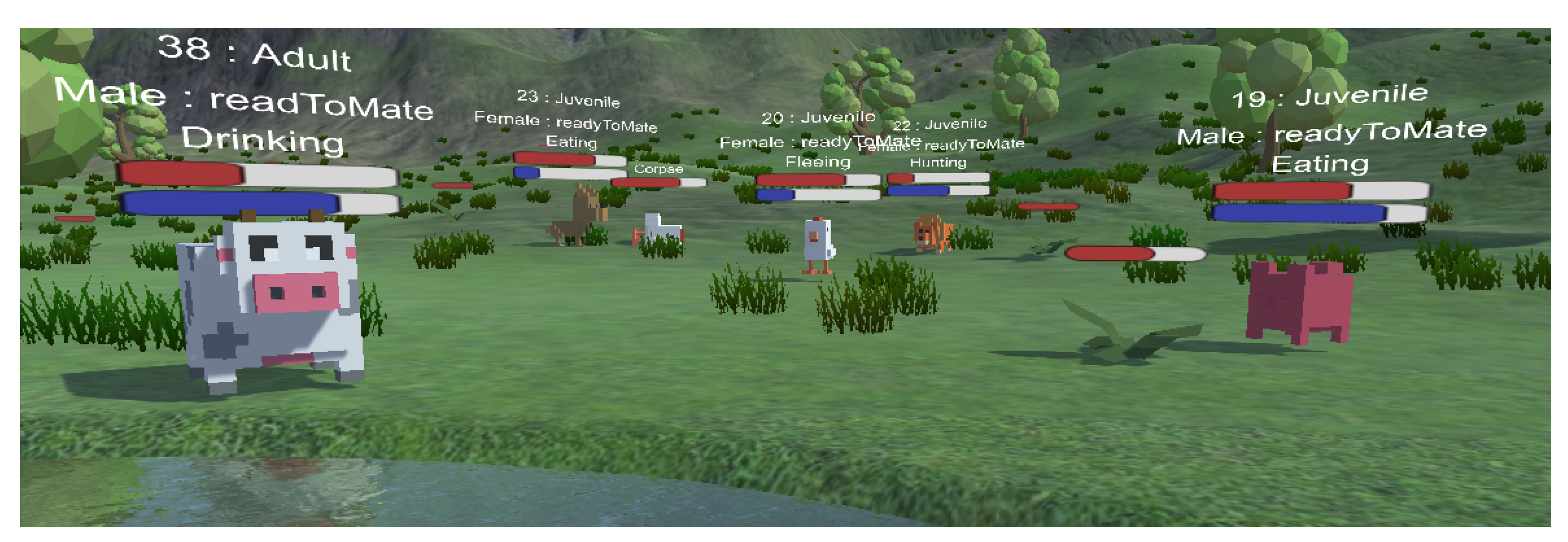
In the simulation to imitate the metabolism effect, the animals have a thirst and hunger meter which must be maintained, otherwise, the animal will become deceased. When an animal is thirsty and a water source is found, the animal can drink from the water, replenishing its thirst meter. If the animal is hungry and a food source is found, in case the animal is herbivorous, a simple eating mechanics starts. If the animal is carnivorous and a living prey is found, then a hunting mechanics is triggered and the animal starts to pursue and try to catch its target. The prey can detect its predator and will begin a fleeing mechanic to try to outrun its pursuer. If the prey is faster, it can outrun the predator, but if the predator catches it, then the same eating mechanics starts, where the recently deceased prey will be the food source for the predators. These phases have a strong effect on other animals’ phases (Figure 6) because the different species are in the same closed simulation environment.
We further enhanced our simple predator–prey model with a simplified aging mechanic (Figure 7), which changes the attributes of the animals while time progresses and the animals age. In the program, we determined some different age stages for the animals, where we can set the specific attributes for every stage. In our sample, animals started in a “Puppy” age stage, where their attributes were lower, next was “Juvenile”, followed by “Young”, where their skills gradually improved, followed by the “Adult” stage, where the animals had the best attributes. From this point, the animal started getting older with “Aged” and “Elder”, where the attributes were lowered. The stage borders were determined by a percentage-based distribution relative to the species’ average lifespan. With the animal’s age approaching the end of the lifespan, the animal is more likely to die unexpectedly, representing natural sudden death due to its old age.
One of the most intriguing model enhancements is the mating system (Figure 8), which is responsible for the reproduction process of the animals. Except for the starting animals in the simulation which are set by the user, all animals are born by their parents. When animals reach maturity they become sexually active and if a male and a female from the same species meet, then they can mate and create offspring. After the mating process, the female becomes pregnant (Figure 9). While the females are carrying their babies, their metabolism processes accelerate and they require more water and food. If the female gets through the hard pregnancy period, whose length is controlled by a pregnancy duration attribute, she gives birth to her children. The children start in a special “Newborn” age stage right after birth, which only lasts for a very short duration. After that, they become “Puppys” and start living their childhood.
There is an optional mechanic, which is the pack forming mechanic (Figure 10). If the animals have the ability to form packs, they can stick together forming groups and moving together on the terrain. In our previous work [1] we looked thoroughly into the advantages and disadvantages of this behavior type. The pack mechanic has a strong benefit in the mating process, because the animals stick together, therefore the distance between animals is short, and the search time for a suitable mate is lowered drastically. In addition, it could improve the lifetime and the survival chances, but as a disadvantage, the local food consumption speeds up and the pack can be cornered faster and easier. Every group has a leader who is the oldest member in the pack. The leader can set a specific direction, and every member will move slightly in that direction following the leader resulting in a coordinated pack movement during exploration. This movement pattern is broken only if an enemy is nearby. In that case, the members will run separately until the danger disappears. Afterward, they will try to rejoin their pack. The packs are formed by individuals joining or even leaving packs (animals always try to form bigger packs until a limit). When a new child is born, then it is added to its parents’ pack automatically.
3.3. Flaws of the Model
There are limitations and disadvantages of the previous model. In the simulation, a large number of attributes have to be set manually for every species in every age stage. This makes it difficult to operate the software and difficult to achieve a balanced simulation. Another problem is the simplified reproduction process, since the animals and their offspring have exactly the same attribute values, and thus the offspring will be the perfect clones of their parents. In the multi-species food-chain predator–prey model, balancing is more difficult. During the simulation, many events can occur, such as the extinction of prey species, which is difficult to predict, and if the animals always have the same attributes in the simulation, they may not be able to survive the extreme effects. Although in this simplified simulation model, predators would not be able to survive the global, sudden extinction of populations of prey species, they could still be saved if they did the same thing as humans try to protect endangered species. When predators suffer from food shortages, slower metabolism can help them get through difficult times until prey populations stabilize, and if prey species can improve their reproduction rates in a crisis, then they can accelerate the population recovery process.
4. Our New Extended Simulation System Using Gene Evolution
We created an evolutional approach to the model, where the species still have their predetermined attributes as starting points, which change as they age, but some of the attributes can evolve. Every animal has a simplified gene model, which alternates its default attributes. When two individuals (parents) with different gene structures create offspring, then their genes are combined together according to a simplified Mendel-inheritance model. This new gene creation is determined and set when the child is born. Every sibling has a different mixed gene structure originating from their parents making every child unique from the other siblings and their parents. Genes are determined with value-pair dominant and recessive values in every gene type. The dominant is the better value inherited from parents matching gene type, while the recessive is set by the second best. However, while the animals’ gene structures are changing, their skills do not surpass their parents’ set attribute values. Additionally, in order to evolve the values from the gene mixing process, genes can mutate, making the genes’ value randomly better or worse. This makes every generation of animals different from the other, and every generation contains a large variety of animals with different attributes.
With the natural selection in an ecosystem, the fittest animals can survive. The fittest is always determined by the current state and situations of the ecosystem. While the ecosystem is constantly changing, animals need to adapt. Without the animals knowing exactly what is the best attributes for the current state, they can only “guess”, meaning they have to create several children and hope at least one of them is evolved in such a way that may enable that they can survive to create offspring on its own, making an ever adaptive generational link. For example, if the predator population is low, the prey’s population will grow and consume nearly all the food on the map, resulting in a food shortage for them. The natural response would be to improve the metabolism ability to survive, but while they do this, the predators may start to improve their speed capabilities. If the predators become much faster than the prey, then they can catch them more frequently and if they have a bad metabolism (because they improved their speed and not the metabolism rate), then they can and will hunt down the majority of the prey to satisfy their needs. If they overhunt the prey, then the opposite occurs, and predators will have a food-shortage problem. If they respond correctly and increase their metabolism to adapt to the low scattered food resources, then they can survive, and thus—due to the lack of predation pressure—allows the prey population to rebound, but in the meantime, a lot of predators will become deceased. With the low predator population, we arrived back to the starting point of the example. This means that both parties periodically try to balance their population over time, resulting in an adequate (extinction-resistant) predator–prey fluctuation.
The previous example described a well-balanced system, but most of the time, this is not so simple, because if the predators behave really aggressively and dominantly, and if the prey population is low, then they might not increase their metabolism, rather their speed to compete with each other for food. This will result in a catastrophe because they will continue hunting down the already few remaining prey to extinction. This is the same with the prey if they compete with each other for the vegetation by developing their speed capabilities, then they sentence themselves to extinction. On the other hand, if they increase their metabolism rate only until the vegetation can sustain the current prey population, then they can start to increase their speed, but they do not start to compete, instead, they start to increase their survival rate. With bigger speed values they have a better survival chance against the predators’ attacks, while an excellent metabolism value does not help in this kind of situation. Consequently, the animals always have to adapt to their current situation, where the less compatible animals die, the fitter animals can more likely survive and can pass on their gene structure to future generations.
5. Our New Model and Its Implementation in the Simulation System
We have kept everything from the original [1] framework, and in the new model we have added the new gene system, have reworked the animal properties system, and have adjusted the afflicted aging and mating systems. The old system directly used the attribute values from the aging and mating system, but now their values are calculated from the default and the evolution values. We chose three attributes as a demonstration to upgrade them to generative traits called Gene Types. With the new gene system, these attributes are altered constantly during the simulation. Any other animal attributes in the simulation can be extended with the evolutional process for further experiments. Speed (Figure 11) affects the ability to travel faster. Metabolism (Figure 12) controls how fast the animal burns energy over time. Pregnancy (Figure 13) determines how long it takes for the females of the species to produce offspring.
The Speed and Metabolism values kept their changing nature with the predetermined different age group setting. To these values, we recalculate the final attribute values by adding together the original age setting value and the corresponding gene value. The pregnancy time is an exception because it is an unchanging attribute, which means that it is determined by adding the constant mating system’s value for the species and the Pregnancy gene value together.
5.1. Inheritance
At the start of the simulation, the spawned animals start with neutral Gene Structure (), which means the Dominant () and Recessive () values are 0 in each gene types because they do not have previous ancestors to inherit values from. This way we assume that their ancestors have had some unknown values, which would result in a special generation with neutral gene structures, representing a base to the future comparisons. If we still wanted to start the simulation with different animals, whilst the starting animals cannot inherit, then they can mutate without a problem. This way all the spawned animals are already different slightly from each other. These stating animals are called the first generation. After the first generation, the newborns’ gene values come from a random combination of the parents’ gene pool (Figure 14), which will also mutate after the inheritance.
In the inheritance process, the father’s gene structure () and the mother’s gene structure () are combined together, where every offspring randomly gets one of the values from the father’s dominant and recessive () and the mother’s () gene pair, as () and () values. This inheritance process is calculated for each gene type. A child could get two great values from both parents, resulting in the fittest offspring, but it could equally result in any combination.
In every gene type, it can be set how the two values are assigned to the dominant and recessive alleles. When they inherited these two values, one of them will be the dominant and the other is the recessive gene value. In the simulation, we need only one value and we used the dominant one to represent the ability of the individual, while the recessive gene will be a hidden allele. The choice is determined by an Inheritance Priority () attribute, where we can set which value will be the dominant one, and therefore we used as the animal’s value property in the simulation. Let x be the bigger and y the smaller values of and .
5.2. Mutation
After the inheritance process, the calculated gene pairs in each gene type can mutate in different ways. The mutation process can be controlled by two main parameters. The first is the Mutation Type () category option, which determines what values can mutate. Its value will be a random number within a given Mutation Min () and Mutation Max () range. If the is negative and the is positive, the mutation process can randomly enhance or diminish the inherited value. If both are negative or positive, then the mutations will have a straightforward effect on the values. The second parameter is the Mutation Probability () value. It helps to manipulate the possibility of whether the offspring mutates the inherited value or it does not. Lower will slow down the evolutional process and the animals will be much more identical, while bigger have a much more drastic impact on the generations.
5.3. Generations
Every animal has a generation counter, which is similar to a family tree, where the number represents the depth of the offspring’s family tree. The starting animals are always the first generation, but after that, any child’s generational number is calculated by the average of the parents’ generations + 1. This way the tree’s depth represents the generational link from the first generation without following any male- or female-line generation types.
6. Experiments
We would like to emphasize that we have made the system publicly available for further research. Anyone can use it to simulate their own ecosystem, to simulate the fauna and flora of any smaller or larger closed environment (from islands to continents) over time. Anyone can define any number of their own animals and plants, specify the size of the initial populations, define relationships between living things (such as food chains, hereditary relationships), and even customize many other characteristics. After starting the simulation, the migration, hunting, and reproduction of the animals and species can be observed visually and events can be identified, which can be further analyzed as the simulation data are saved in a database. This can help in research on sustainability, overpopulation, migration, and species extinction. It is possible to support hypotheses by simulation, as well as forecasts and risk analyses of the ecosystem. To demonstrate how our system can be used, we provide a simulation and examination of simulated data from a few aspects, but the number of case studies like this is innumerable.
For demonstration purposes, we show two simulations that we ran in the framework. As a comparison to show the influence of the gene evolution system, we ran two simulations with identical parameters (environment, species, attributes, and so on), and with the gene evolution system turned on and off. The datasets and the results of these two simulations are published alongside the program code on Github [41]. In the simulation, we used illustrative entities with sample attribute values that do not have any relations with real-life entity attributes. As the low end of the food chain, we used one plant species named “Grain” as map-wide vegetation. The vegetation type is a special entity in the predator–prey model, serving as a food source for the herbivore prey animals. These vegetation entities differ from animals in a way that they cannot move or evolve. We created a herbivore prey animal named “Chicken”. These prey animals can move on the ground and flee from predators, reproduce, evolve and as nourishment, they eat the vegetation available on the map. We created the “Dog” and “Lion” animals as predators that hunt the prey. The “Dog” animals are smaller and more prolific than “Lion” animals. The latter ones are on the top of the food chain hunting both “Chicken” and “Dog” species and have no natural enemy.
6.1. Attributes
The three animal types all have the three sample gene types (Speed, Metabolism, Pregnancy) and they inherit their genes based on the described model in Section 5. The starting attribute values can be seen in Table 1 which are not affected by the aging mechanics and in Table 2 which are affected and shown by age stages.
During the examination, the gene pools of the newborn and the gene pools of the parents were saved at the moment of birth of the offspring. As the offspring may be born with better or worse values, we have decide that the parents are the ones who should be monitored for natural selection rather than the newborns, because they are the ones who have already proven that their gene pool is suitable for the given situation as they have survived maturity and created offspring.
6.2. Basic Population Analysis
The simulations begin by spawning a specified number of entities (180 pieces of grain, 150 chickens, 50 dogs, and 15 lions) on the map. The animals begin as newborns in random places, with their attributes automatically set to their species’ attributes at their present age stage.
In Figure 15, we can see the overall population fluctuation of the species with the gene evolution system turned on. The graphs show how quickly the populations can fluctuate due to many factors. Because the Chickens were the only prey population, they had a rapid reproduction rate and sustained a much higher population than the other species. During their rapid population growth, the chickens consumed nearly all the available grain on the map in the 801–1700 period and started to have a food shortage (also check Figure 16 for chicken deaths from hunger). This means that starvation had an extraordinary dominant effect on controlling the population.
Figure 15 and Figure 17 show the difference between the new gene evolution system turned on and off. The vertical axis shows the population and the horizontal axis shows the simulation time in seconds, displayed in 100-s interval categories. On the left we can see Dog/Lion/Grain as a lower population species and on the right, Chicken, with a much higher population than the other species.
Next, in addition to the population numbers, the mortality distribution of the animals (cause of deaths) is shown for each species separately, which presents how many animals died due to the observed factors (Death by Thirst, Hunger, Age, or Predators) at the given simulation interval.
Figure 16 and Figure 18 show the difference between the new gene evolution system turned on and off. The vertical axis shows the population and the horizontal axis shows the simulation time in seconds, displayed in 100-s interval categories. On the left, we can see Thirst/Predator/Age as a lower determining cause factor, and on the right, Hunger, which is a 10 times higher cause for deaths in the evolution system than other causes.
Due to the high prey population, the predator population started to grow as well. First, the dog population started to grow because they had a much faster reproduction rate (401–2500 period). At the same time, the lions’ population started to grow as well due to the adequate food supply. The dogs began to lose territory, and their and the lions’ population sizes shifted (about at 3401–3500). This demonstrates how competing predator species, when one may hunt the other, can have an impact on the population of the weaker side. However, this was not due to overhunting; according to Figure 19, the problem (in addition to aging) was thirst, not predation. In the simulation, the lions did not always hunt the dogs since they had enough food, but the dogs were naturally running from the lions when the lions were scattered or occupied key locations. These key areas could be like water sources, and prey hunting grounds. The lions could easily shut out the dogs by frightening them away from these important areas, therefore causing them to die due to thirst and hunger.
Figure 19 and Figure 20 show the difference between the new gene evolution system turned on and off. The vertical axis shows the population and the horizontal axis shows the simulation time in seconds, displayed in 100-s interval categories. On the left, we can see Thirst/Hunger/Predator as a lower determining cause factor, and on the right, Age, which is a 4 times higher determining cause in the evolution system than other causes.
In the simulation with the gene evolution system turned on, the dogs became extinct (at about 5201–5300 ), which let the chickens’ population grow rapidly. In case we check the cause of deaths of the lions (Figure 21), we can observe that the rate of the causes does not vary with or without the presence of competing dogs in the food chain since the dogs were less influential in the food chain. As the lion population increases and the dog population declines, the territory hostility for chickens is hardly changed. The lions could continue the hunting, but only on chickens, which had an acceleration effect on their starvation condition, and the chicken population started to grow rapidly.
Figure 21 and Figure 22 show the difference between the new gene evolution system turned on and off. The vertical axis shows the population and the horizontal axis shows the simulation time in seconds, displayed in 100-s interval categories. On the left, we can see Thirst/Hunger/Predator as a lower determining cause factor, and on the right, Age, which is a 10 times higher determining cause in the evolution system than other causes.
6.3. Gene Evolution
We set all genes’ mutation probability to 100% and the Mutation (minimum, maximum) as Speed (−0.15, 0.15), Metabolism (−0.1, 0.1) and Reproduction (−0.4, 0.4). The crucial aspect of the simulation was that we set the mutation range symmetrical to 0 so that when a new child is born, its mutation value can be either negative or positive, implying that the newborns’ characteristics might be better or worse than their parents. We show the average of these mutation values in Figure 23 in every generation. When the number of average mutations is close to zero, the animals should keep their original values, but with natural selection the animals who are not fit enough die while the fitter animals survive and inherit their genes, therefore the capabilities of the whole generation are enhanced, as shown in Figure 24. We have drawn a comparison between the new generations’ and their parents’ attributes in Figure 25. We can see that most of the time the new generation had better gene values than their parents.
The demonstration simulation which uses our new gene evolutional model shows that the animals have the tendency to improve their skills due to the natural selection process, which can ensure that the animals are ever-evolving towards a more adaptive, fitter state in the long term.
7. Further Use Cases
One of the strongest features of graphical frameworks is the eye-catching experience. This kind of 3D simulation has a wide area of uses beyond the regular ones. Regular simulations are excellent for creating scientific predictions and analytic statistics, but they do not support the user to obtain the meaning and experiences of the system. On the other hand, 3D animated simulations are helpful for creating ecological showcases for audiences, such as students in schools, or they are proper for presentations. At schools, students can monitor a wide variety of events and behaviors of the animals in real-time by graphical observation. They can learn how the prey animals react to danger or cooperate in packs while living their life in the simulation. To make the class more interactive, students can be involved in the simulations when teachers define a simulation “world” with instructional scenarios, and the students can create a different imaginary animal species with diverse attribute parameters and run simulations. The students can hold a competition and vote on what species will survive the longest, or which predator is the most efficient, and so on.
8. Conclusion and Future Works
Ecosystem simulation research and development are significant assets for ecology improvement since these frameworks provide a number of benefits, such as tracking the evolution of individual species, changes in population quantity, quality, and different ratios through time. Further opportunities for the system usage include prediction of endangered species extinction, as well as possible prevention or improvement due to artificial colonization and predicting natural disasters’ environmental impacts like climate change, earthquakes, and sea-level rise.
In this article, we have shown how to extend our system of 3D ecosystem simulation based on the predator–prey model with inheritance. Having the gene evolution algorithms built into the system, it more effectively models the ecological environment, than the old, non-evolutional version of the framework. Simulations can generate simulation data for further ecosystem research (sustainability, overpopulation, species extinction, migration) that are easier to interpret due to the appearance of 3D.
The model in some aspects is rather simple, therefore we present some ideas for further improvements in the model, for example, animal behaviors and optimization areas for conducting simulations with bigger populations, user interfaces for easier program usage.
As a model improvement, more gene types could be created to polish more of the animals’ adaptation ability. We plan to implement more mechanics in animal behaviors, framework features, and monitoring, exporting, and analyzing more data for various studies. We intend to improve and optimize some of the existing mechanics, such as more complex escape strategies for the prey, in which the animal considers all enemies and their distances and terrain formations and calculates the appropriate vector. Furthermore, redesigning the animal’s view mechanism would be more efficient.
We are planning to implement a role mechanism, which would imply that different tasks (such as hunter, explorer, and so on) may be assigned to animals within packs depending on their exceptional talents (using the new gene system). Smaller animals will have the capability to hide from predators in certain areas (such as bushes or nests). New sleeping mechanics and day–night cycles can also be considered. The model can be extended by a new family mechanics which has a greater and stronger impact on the decision-making capability than the current pack system has. For example, if a family member is in a hard situation (such as an attack), the pack (the family) will aid the individual immediately, even risking their lives, or the older members may give or share food with the younger ones in case they are hungry to a critical extent. Another way to extend the model is introducing a basic type of communication (information transmission) among family, pack and race members in order to exchange location information, such as food and water locations, dangerous regions, even basic planned hunting processes, for example, approaching and encircling the prey collectively.
Moreover, more sophisticated fighting mechanics could be defined that replaces the predators’ existing immediate killing hunting mechanics. This would create a new vitality meter (in addition to hunger and thirst meters), which would display whether the animal is full of energy (i.e., not thirsty, hungry, or injured) or depleted, and this could influence other states, such as the amount of damage they receive and inflict on others. When an animal takes an injury or has a low energy level, they begin to lose attribute value, such as speed, until the energy level reaches an ideal level, at which point the attribute will slowly be restored to its previous value. A new combat system may be built using this new fighting mechanism, such as intra-species battles over food or females, or during a hunt, a duel can be performed where the prey can attack back instead of fleeing (making a damage system that drains both competitors’ life force), or where one of the animals can choose to flee if his life level is low. If there are other animals in the area, then they can decide to aid. If a lot of prey form a band to fight back, then they could chase away or even kill a single predator, thus the predators may not always win the fight, and species without a natural enemy could also be in danger not just from hunger and thirst, but from other rallying species.
Multiple user features could improve the usage of the program, such as an animal customization interface that would allow users to create new species and alter their attributes within the software. Currently, these can be specified in a configuration file, not interactively. These new species may be used in the custom simulations and may be saved for future simulations. Instead of utilizing simply heightmaps, users could use new randomly or procedurally created maps like Perlin noise [42] and other noise types merged.
We believe that the current system is also capable of simulating simplified ecosystems, providing a simulation framework for a wide variety of research, and with the above possible improvements, even finer modeling and even more accurate predictions could be made.
Author Contributions
Conceptualization, G.P. and A.K.; methodology, G.P. and A.K.; software, G.P.; validation, G.P. and A.K.; investigation, G.P. and A.K.; writing—original draft preparation, G.P. and A.K.; writing—review and editing, G.P. and A.K.; supervision, A.K.; project administration, A.K.; All authors have read and agreed to the published version of the manuscript.
Funding
The project has been supported by the European Union, co-financed by the European Social Fund (EFOP-3.6.3-VEKOP-16-2017-00002). This research was also supported by grants from the “Application Domain Specific Highly Reliable IT Solutions” project that has been implemented with the support provided by the National Research, Development and Innovation Fund of Hungary, financed under the Thematic Excellence Programme TKP2020-NKA-06 (National Challenges Subprogramme) funding scheme.
Institutional Review Board Statement
Not applicable.
Data Availability Statement
The demonstration experiment’s sample data which were used in this article [41] and framework [43] can be found on a Github repository. The project can be freely downloaded, expanded, and changed for personal use. Visit the browser version [44] to try out and experience a live version of the software without any installation.
Acknowledgments
We would like to thank Judit Juhász for her contribution to correcting the text.
Conflicts of Interest
The authors declare no conflict of interest.
References
- Kiss, A.; Pusztai, G. Animal Farm—A complex artificial life 3D framework. Acta Univ. Sapientiae Inform. 2021, 13, 60–85. [Google Scholar] [CrossRef]
- Lotka, A.J. Elements of Physical Biology; Williams & Wilkins: Philadelphia, PA, USA, 1925. [Google Scholar]
- Volterra, V. Lecons sur la Theorie Mathematique de la Vie; Gauthier-Villars: Paris, France, 1931. [Google Scholar]
- Berryman, A.A. The orgins and evolution of predator–prey theory. Ecology 1992, 73, 1530–1535. [Google Scholar] [CrossRef] [Green Version]
- Abrams, P.A. The evolution of predator–prey interactions: Theory and evidence. Ann. Rev. Ecol. Syst. 2000, 31, 79–105. [Google Scholar] [CrossRef]
- Wright, S. Evolution in Mendelian populations. Genetics 1931, 16, 97. [Google Scholar] [CrossRef]
- Wright, S. Isolation by distance under diverse systems of mating. Genetics 1946, 31, 39. [Google Scholar] [CrossRef]
- Falconer, D.; Mackay, T. Introduction to Quantitative Genetics; Longmans Green: Harlow, UK, 1996; Volume 3. [Google Scholar]
- Leroy, G.; Mary-Huard, T.; Verrier, E.; Danvy, S.; Charvolin, E.; Danchin-Burge, C. Methods to estimate effective population size using pedigree data: Examples in dog, sheep, cattle and horse. Genet. Select. Evol. 2013, 45, 1–10. [Google Scholar] [CrossRef] [Green Version]
- Nomura, T.; Yonezawa, K. A comparison of four systems of group mating for avoiding inbreeding. Genet. Select. Evol. 1996, 28, 141–159. [Google Scholar] [CrossRef]
- Silva, L.d.C.; Cruz, C.D.; Moreira, M.A.; Barros, E.G.d. Simulation of population size and genome saturation level for genetic mapping of recombinant inbred lines (RILs). Genet. Mol. Biol. 2007, 30, 1101–1108. [Google Scholar] [CrossRef] [Green Version]
- Beckett, T.J.; Rocheford, T.R.; Mohammadi, M. Reimagining maize inbred potential: Identifying breeding crosses using genetic variance of simulated progeny. Crop Sci. 2019, 59, 1457–1468. [Google Scholar] [CrossRef]
- Windig, J.J.; Hulsegge, I. Retriever and pointer: Software to evaluate inbreeding and genetic management in captive populations. Animals 2021, 11, 1332. [Google Scholar] [CrossRef]
- Mendel, G. Versuche über Pflanzenhybriden; BoD–Books on Demand: Norderstedt, Germany, 2020. [Google Scholar]
- Henig, R.M. The Monk in the Garden: The Lost and Found Genius of Gregor Mendel, the Father of Genetics; Houghton Mifflin Harcourt: Boston, MA, USA, 2000. [Google Scholar]
- Darwin, C.; Wallace, A.R.; Lyell, S.C.; Hooker, J.D. On the Tendency of Species to Form Varieties: And on the Perpetuation of Varieties and Species by Natural Means of Selection; Linnean Society of London: London, UK, 1858. [Google Scholar]
- Darwin’s, C. On the Origin of Species; Hachette UK: London, UK, 1859; Volume 24. [Google Scholar]
- Spencer, H. The Principles of Biology: Volume 1; Outlook Verlag: Freiburg im Breisgau, Germany, 2020. [Google Scholar]
- Fisher, R. The Genetical Theory of Natural Selection; The Clarendon Press: Oxford, UK, 1930. [Google Scholar]
- Bowler, P.J. The Eclipse of Darwinism: Anti-Darwinian Evolution Theories in the Decades around 1900; JHU Press: Baltimore, MD, USA, 1992. [Google Scholar]
- Bowler, P.J. Evolution: The History of an Idea; University of California Press: Berkeley, CA, USA, 1989. [Google Scholar]
- Ulett, M.A. Making the case for orthogenesis: The popularization of definitely directed evolution (1890–1926). Stud. Hist. Philos. Sci. Part C Stud. Hist. Philos. Biol. Biomed. Sci. 2014, 45, 124–132. [Google Scholar] [CrossRef] [PubMed]
- Huxley, J.; Pigliucci, M.; Muller, G.B. Evolution. The Modern Synthesis; The MIT Press: Cambridge, MA, USA, 1942. [Google Scholar]
- May, R.M. Limit cycles in predator–prey communities. Science 1972, 177, 900–902. [Google Scholar] [CrossRef] [PubMed] [Green Version]
- May, R.M. Will a large complex system be stable? Nature 1972, 238, 413–414. [Google Scholar] [CrossRef] [PubMed]
- Gilpin, M.E.; Rosenzweig, M.L. Enriched predator–prey systems: Theoretical stability. Science 1972, 177, 902–904. [Google Scholar] [CrossRef] [Green Version]
- Luck, R.F. Evaluation of natural enemies for biological control: A behavioral approach. Trends Ecol. Evol. 1990, 5, 196–199. [Google Scholar] [CrossRef]
- Arditi, R. The biological control paradox. Trends Ecol. Evol. 1990, 6, 32. [Google Scholar] [CrossRef]
- Begon, M.; Sait, S.M.; Thompson, D.J. Predator–prey cycles with period shifts between two-and three-species systems. Nature 1996, 381, 311–315. [Google Scholar] [CrossRef]
- Rosenzweig, M.L. Evolution of the predator isocline. Evolution 1973, 27, 84–94. [Google Scholar] [CrossRef]
- Rosenzweig, M.L.; Schaffer, W.M. Homage to the Red Queen. II. Coevolutionary response to enrichment of exploitation ecosystems. Theoretic. Popul. Biol. 1978, 14, 158–163. [Google Scholar] [CrossRef]
- Rosenzweig, M.L.; Brown, J.S.; Vincent, T.L. Red Queens and ESS: The coevolution of evolutionary rates. Evol. Ecol. 1987, 1, 59–94. [Google Scholar] [CrossRef]
- Abrams, P.A.; Matsuda, H. Prey adaptation as a cause of predator–prey cycles. Evolution 1997, 51, 1742–1750. [Google Scholar] [PubMed]
- Cortez, M.H.; Patel, S. The effects of predator evolution and genetic variation on predator–prey population-level dynamics. Bull. Math. Biol. 2017, 79, 1510–1538. [Google Scholar] [CrossRef] [PubMed]
- Rufino, M.C.; Herrero, M.; Van Wijk, M.; Hemerik, L.; De Ridder, N.; Giller, K.E. Lifetime productivity of dairy cows in smallholder farming systems of the Central highlands of Kenya. Animal 2009, 3, 1044–1056. [Google Scholar] [CrossRef] [PubMed] [Green Version]
- Bateki, C.A.; Dickhoefer, U. Evaluation of the modified livestock simulator for stall-fed dairy cattle in the tropics. Animals 2020, 10, 816. [Google Scholar] [CrossRef]
- Wang, Q.; Zhang, L.; Zhao, H.; Zhao, Q.; Deng, J.; Kong, F.; Jiang, W.; Zhang, H.; Liu, H.; Kouba, A. Abiotic and Biotic Influences on the Movement of Reintroduced Chinese Giant Salamanders (Andrias davidianus) in Two Montane Rivers. Animals 2021, 11, 1480. [Google Scholar] [CrossRef]
- Unity (Game Engine). Available online: http://www.unity3d.com/ (accessed on 11 November 2021).
- Lind, J.; Enquist, M.; Ghirlanda, S. Animal memory: A review of delayed matching-to-sample data. Behav. Process. 2015, 117, 52–58. [Google Scholar] [CrossRef]
- Many Animals—Including Your Dog—May Have Horrible Short-Term Memories. Available online: https://www.nationalgeographic.com/animals/article/150225-dogs-memories-animals-chimpanzees-science-mind-psychology (accessed on 11 November 2021).
- Github Demonstration Experiment Data Samples, Which Was Used to Create the ‘Demonstration Experiment’ Section. Available online: https://github.com/Wornox/AnimalFarmFramework/tree/main/Research (accessed on 11 November 2021).
- Li, H.; Tuo, X.; Liu, Y.; Jiang, X. A parallel algorithm using Perlin noise superposition method for terrain generation based on CUDA architecture. In Proceedings of the International Conference on Materials Engineering and Information Technology Applications, Guilin, China, 26–28 June 2015. [Google Scholar]
- Github Project Repository. Available online: https://github.com/Wornox/AnimalFarmFramework (accessed on 11 November 2021).
- Github Runnable Browser Version of the Program. Available online: https://wornox.github.io/AnimalFarmWebGL (accessed on 11 November 2021).
Figure 1.
The framework is divided into four main components with multiple controllers which control the different parts of the program.
Figure 1.
The framework is divided into four main components with multiple controllers which control the different parts of the program.

Figure 2.
One of the sample environments to run the simulations on a medium-sized isolated island with a high land ratio, but plenty of water sources.
Figure 2.
One of the sample environments to run the simulations on a medium-sized isolated island with a high land ratio, but plenty of water sources.

Figure 3.
A sample food-chain relation with different types of species which was used in our previous article. The living entities are organized into chain-levels.
Figure 3.
A sample food-chain relation with different types of species which was used in our previous article. The living entities are organized into chain-levels.

Figure 4.
A simplified representation of the animal’s logic. The top (Start) and bottom (End) ellipses represent the boundaries of the algorithm logic. Rectangles represent the different processes, and diamond shapes represent the requirements of the different phase processes.
Figure 4.
A simplified representation of the animal’s logic. The top (Start) and bottom (End) ellipses represent the boundaries of the algorithm logic. Rectangles represent the different processes, and diamond shapes represent the requirements of the different phase processes.

Figure 5.
Constant exploration is necessary to fulfill the daily requirements, such as thirst and hunger.
Figure 5.
Constant exploration is necessary to fulfill the daily requirements, such as thirst and hunger.

Figure 6.
The circle of life in a predator–prey habitat with usual and everyday metabolism process (eating and drinking) alongside with extreme hunting and fleeing scenarios.
Figure 6.
The circle of life in a predator–prey habitat with usual and everyday metabolism process (eating and drinking) alongside with extreme hunting and fleeing scenarios.

Figure 7.
According to the aging mechanics, animals change over time. The animal’s attributes can be changed in each age stage. We provided a sample setup, where “Newborn” and “Elder” animals have the worst attributes, and “Juvenile” and “Aged” stages also change the sexually active status.
Figure 7.
According to the aging mechanics, animals change over time. The animal’s attributes can be changed in each age stage. We provided a sample setup, where “Newborn” and “Elder” animals have the worst attributes, and “Juvenile” and “Aged” stages also change the sexually active status.

Figure 8.
A simplified representation of the animal’s mating system. The Start and End ellipses represent the boundaries of the algorithm logic. Rectangles represent the different processes, and diamond shapes represent the requirements and decision-making.
Figure 8.
A simplified representation of the animal’s mating system. The Start and End ellipses represent the boundaries of the algorithm logic. Rectangles represent the different processes, and diamond shapes represent the requirements and decision-making.

Figure 9.
The most important event in any organism’s life is the reproduction biological (mating) process for population preservation, in which an organism gives life to young ones (offspring) similar to itself. (a) All species rely on the selection and attraction of a compatible partner to survive. (b) Reproduction ensures the species’ survival from generation to generation.

Figure 10.
The animals can establish packs with other members of their own species. For each race, multiple packs can be formed during the simulation.
Figure 10.
The animals can establish packs with other members of their own species. For each race, multiple packs can be formed during the simulation.

Figure 11.
Animals with a higher speed can outrun any dangerous situations.
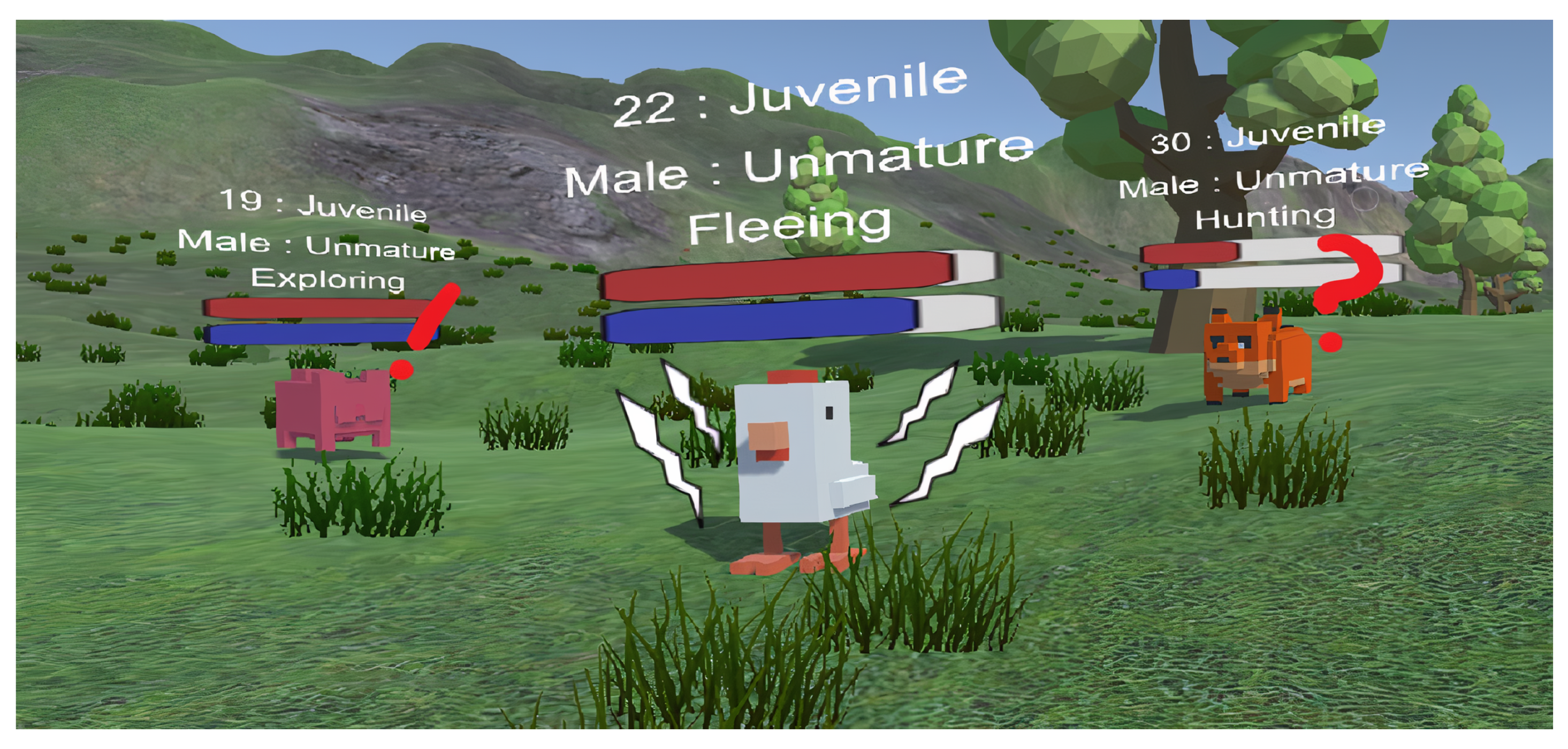
Figure 12.
With a better metabolism animals burn energy slower and consume less food from the environment.
Figure 12.
With a better metabolism animals burn energy slower and consume less food from the environment.

Figure 13.
Animals with a faster reproduction rate create much more offspring than a usually bigger animal with longer pregnancy duration.
Figure 13.
Animals with a faster reproduction rate create much more offspring than a usually bigger animal with longer pregnancy duration.

Figure 14.
The picture illustrates a simple dominant–recessive inheritance pattern with one of the default animal models in the simulation.
Figure 14.
The picture illustrates a simple dominant–recessive inheritance pattern with one of the default animal models in the simulation.

Figure 15.
Population fluctuation during the simulation with the new system.

Figure 16.
The diagram shows the cause of deaths for the Chicken population with the new system.

Figure 17.
Population fluctuation during the simulation without evolution.

Figure 18.
The diagram shows the cause of deaths for the Chicken population without evolution.

Figure 19.
The diagram shows the cause of deaths for the Dog population with the new system.

Figure 20.
The diagram shows the cause of deaths for the Dog population without evolution.

Figure 21.
The diagram shows the cause of deaths for the Lion population with the new system.

Figure 22.
The diagram shows the cause of deaths for the Lion population without evolution.

Figure 23.
The diagram shows the average mutation values during 23 Chicken generations. Because the mutation values are randomly generated within the specified range, they are evenly dispersed as positive and negative mutation effects for every individual, but every generation has a different ratio of mutations.

Figure 24.
The diagram shows the gene types used in the generations. Because of the natural selection effect, all gene types are constantly upgrading in the rate of their mutation range (reproduction had the biggest range).
Figure 24.
The diagram shows the gene types used in the generations. Because of the natural selection effect, all gene types are constantly upgrading in the rate of their mutation range (reproduction had the biggest range).

Figure 25.
The diagram shows a comparison between the new and the old generations. On the vertical axis the parent’s best values were subtracted from the children values. Except for two cases, the new generations had better attributes than their parents.
Figure 25.
The diagram shows a comparison between the new and the old generations. On the vertical axis the parent’s best values were subtracted from the children values. Except for two cases, the new generations had better attributes than their parents.


Table 1.
Default attributes which are not affected by the aging mechanics. Here, only the Pregnancy duration attribute is affected by the evolution system.
Table 1.
Default attributes which are not affected by the aging mechanics. Here, only the Pregnancy duration attribute is affected by the evolution system.
| Attributes | Spawn/ Childbirth | Regen/ Pregnancy Dur. | Limit | Avarage Lifetime | Source for | Food | Enemy |
|---|---|---|---|---|---|---|---|
| Grain | 1/10 s | 1.5%/s | 2000 | Unlimited | Chicken | None | None |
| Chicken | 1–3/labor | 160 s | Unlimited | 750 | Dog, Lion | Grain | Dog, Lion |
| Dog | 1–2/labor | 255 s | Unlimited | 1300 | Lion | Chicken | Lion |
| Lion | 1–3/labor | 390 s | Unlimited | 1300 | None | Chicken, Dog | None |
Table 2.
Default attributes by age stages. Here, Speed and the Metabolism (Thirst/Hunger) are affected by the evolution system. We created the lions with the same attributes as dogs as a rival predator species, with the only exception that the lions can hunt down the dogs, have longer pregnancy, but no natural enemy.
| Attributes | Viewrange | Speed | Metabolism | ||||||
|---|---|---|---|---|---|---|---|---|---|
| Age Stages | Chicken | Dog | Lion | Chicken | Dog | Lion | Chicken | Dog | Lion |
| Newborn | 19 | 20 | 20 | 3.3 | 3 | 3 | 1 | 1 | 1 |
| Puppy | 20 | 23 | 23 | 3.35 | 3.55 | 3.55 | 1.7 | 1.2 | 1.2 |
| Juvenile | 22 | 25 | 25 | 3.65 | 3.85 | 3.85 | 1.9 | 1.3 | 1.3 |
| Young | 23 | 27 | 27 | 4.15 | 4.05 | 4.05 | 2 | 1.4 | 1.4 |
| Adult | 25 | 29 | 29 | 4.35 | 4.2 | 4.2 | 1.9 | 1.3 | 1.3 |
| Aged | 22 | 25 | 25 | 3.75 | 3.7 | 3.7 | 1.65 | 1.1 | 1.1 |
| Elder | 18 | 21 | 21 | 3.25 | 3.2 | 3.2 | 1.15 | 0.7 | 0.7 |
Publisher’s Note: MDPI stays neutral with regard to jurisdictional claims in published maps and institutional affiliations. |
© 2022 by the authors. Licensee MDPI, Basel, Switzerland. This article is an open access article distributed under the terms and conditions of the Creative Commons Attribution (CC BY) license (https://creativecommons.org/licenses/by/4.0/).
Share and Cite
MDPI and ACS Style
Kiss, A.; Pusztai, G. Using the Unity Game Engine to Develop a 3D Simulated Ecological System Based on a Predator–Prey Model Extended by Gene Evolution. Informatics 2022, 9, 9. https://doi.org/10.3390/informatics9010009
AMA Style
Kiss A, Pusztai G. Using the Unity Game Engine to Develop a 3D Simulated Ecological System Based on a Predator–Prey Model Extended by Gene Evolution. Informatics. 2022; 9(1):9. https://doi.org/10.3390/informatics9010009
Chicago/Turabian StyleKiss, Attila, and Gábor Pusztai. 2022. "Using the Unity Game Engine to Develop a 3D Simulated Ecological System Based on a Predator–Prey Model Extended by Gene Evolution" Informatics 9, no. 1: 9. https://doi.org/10.3390/informatics9010009
Note that from the first issue of 2016, this journal uses article numbers instead of page numbers. See further details here.