Design of Position Control Method for Pump-Controlled Hydraulic Presses via Adaptive Integral Robust Control

Abstract

This paper takes the position control performance of pump-controlled hydraulic presses as the research object. The control methods are designed respectively for the two motion stages of rapid descent and slow descent of hydraulic presses in order to improve the control performance of the system. First of all, the accuracy model of the pump-controlled hydraulic presses position servo system (the pump-controlled hydraulic presses position servo system, which is called PCHPS) and its MATLAB/Simulink simulation platform are established. Based on the theoretical analysis and experimental data, the interference factors affecting the tracking accuracy and positioning accuracy of the PCHPS are analyzed. Then, an adaptive integral robust control (the adaptive integral robust control, which is called AIRC) for PCHPS is designed to reduce the influence of nonlinear factors on the system, and the effectiveness of the controller is verified by simulation. Finally, the position control experiment of PCHPS is designed, and the experimental results show that the AIRC can effectively reduce nonlinear factors such as unknown interference in the slow-down stage of the system. The positioning accuracy is raised to within 0.008 mm, which improves the process level of the hydraulic presses.

1. Introduction

In the hydraulic transmission equipment used in the production of forgings, hydraulic presses [1,2,3,4] have been widely used in automobile manufacturing, aerospace, warships, and other industries. However, the lack of advanced control methods not only leads to the decline of hydraulic presses process level and energy utilization but also brings great energy consumption loss [5,6,7]. It can be seen that improving the process level of hydraulic presses and optimizing the control performance of the pump-controlled hydraulic presses position servo system (the pump-controlled hydraulic presses position servo system, which is called PCHPS) are of great practical significance to promote the growth of production capacity in their application fields and improve economic efficiency.

In the past, many researchers have paid attention to the control problem of the electro-hydraulic system. Due to its simplicity and ease of implementation, the proportional–integral–derivative (PID) control is still widely applied in industry today. However, in order to deal with the nonlinear phenomenon in the system, fuzzy control is an intelligent control method that imitates the human logic thinking and is independent of the accurate mathematical model of the controlled plant [8]. Macchelli A. illustrate the design and the simulative validation of an adaptive controller developed for an hydraulic presses. By using singular perturbation arguments, they show robustness to slowly increasing leakage gains, which is a typical situation in a real-world application [9]. As far as the hydraulic control system [10], the traditional control strategy is often designed and optimized based on the linear framework, usually by linearization processing near the balance point of the system mathematical model, and by analyzing the system transfer function and configuring the proper and reasonable feedback gain or design correction compensation link to deal with various interferences and parameter perturbation. However, the nonlinear factors prevalent in hydraulic systems cannot be ignored; for example, the non-linearity of differential formula structure in mathematical mechanism modeling, the parts of the model that cannot be modeled accurately, such as load interference, leakage, or the uncertainty of model parameters, changes in load quality, hydraulic elastic modulus due to wear and temperature, etc. [11,12]. The limitations of the traditional linear control strategy cannot cover and deal with these nonlinear factors. In recent years, various nonlinear control methods have been applied in the motion/speed control problem of the electro-hydraulic system. Among them, the adaptive control and the sliding mode control are thought as two effective and alternative methodologies for the nonlinear controller design of the electro-hydraulic system. Xuanjudan proposes an incomplete differential-based improved adaptive backstepping integral sliding mode control to realize the position control for the hydraulic servo system based on the friction compensation. The backstepping-based control integrated with the integral sliding mode surface-based sliding mode control with the friction compensation is used to solve the problem of non-structural uncertainty of the hydraulic system. The incomplete differential is introduced to the adaptive update law by which the low-pass filtering behavior in the incomplete differential is capable of effectively suppressing the interference caused by the pure differential mutation signal [13]. Chong Chee Soon deals with an evaluation on the designed controller named as sliding mode control in which the sliding surface of the controller has been integrated with a proportional–integral–derivative controller. The control scheme is established from the derived dynamic equation, whose stability is proven through Lyapunov theorem [14]. However, the significant drawback of adaptive control is that the transient performance is commonly unknown, and the ability to resist disturbance is normally poor. Although some modifications may be employed to enhance the system robustness, tracking accuracy can no longer be guaranteed. Unlike adaptive control, the SMC can achieve a guaranteed transient performance and final tracking accuracy through robust feedback in the presence of both parametric uncertainties and uncertain nonlinearities. However, the biggest disadvantage of sliding mode control is that it usually involves high-frequency switching in control signals, which may result in control chattering. Although some smoothing techniques may be adopted to reduce the control chattering, the tracking performance is degraded. Therefore, it is of great research value to deal with the nonlinear factors in the pump-controlled system and design the nonlinear control method to improve the control performance of the system.

In this paper, the mathematical mechanism modeling and analysis of PCHPS are studied, and a reasonable simplified mathematical model is applied in the subsequent motion controller design. Aiming at the nonlinear factors such as unknown disturbance and the parameter uncertainty of the hydraulic presses model, an adaptive robust controller is designed based on the simplified mathematical model. Considering that the slow-down and fast-down motion stages have a great impact on the hydraulic presses position control system, a PCHPS position control based on an adaptive integral robust control algorithm is proposed, and the effectiveness of the controller is verified by simulation. Finally, the position control experiment of PCHPS is designed, and the control effect of the designed adaptive integral robust controller is verified and theoretically analyzed. The experimental results show that the adaptive integral robust control algorithm can effectively reduce the influence of nonlinear factors such as unknown interference in the slow-down stage of the system, The influence of nonlinear factors such as unknown interference and parameter uncertainty on the system is reduced, and its position tracking accuracy is improved.

The rest of this paper is organized as follows. The second section describes the problem formulation and dynamic models. The third section is the design and simulation of adaptive robust motion controller. The fourth part is the setting and results of the experiment. Conclusions are drawn in the last section.

2. The Mathematical Model and Analysis of PCHPS

2.1. The Principle of PCHPS

The hydraulic principle of PCHPS is shown in Figure 1. In Figure 1, element 1 is the coarse oil filter, element 2 is the servo motor, element 3 is the hydraulic pump, element 4 is the servo driver, element 5 is the rotary encoder, element 6 is the check valve, element 7 is the fine filter, element 8 is the overflow valve, element 9 is the hydraulic controller, element 10 is the magnetic exchange valve, element 11 is the balance valve, element 12 is the charge valve, element 13 is the pressure transducer, element 14 is the hydraulic cylinder, and element 15 is the displacement transducer.

The PCHPS is shown in Figure 1, where the action of the hydraulic cylinder can be divided into the following working stages:

(1)

Fast-next stage: The electromagnetic directional valve 1DT, 3DT, and 4DT are powered, and the hydraulic oil enters the small cross-sectional area of the hydraulic cylinder. The hydraulic cylinder is driven to complete rapid movement with small flow, and it finally returns to the oil tank.

(2)

Slow-down stage: The electromagnetic directional valve 1DT is powered, the hydraulic oil enters the rodless cavity of the hydraulic cylinder to push the hydraulic cylinder to complete the slow motion with a large flow.

(3)

Position-holding stage: The electromagnetic directional valve 1DT is powered, the motor speed will be adjusted in real time according to the position parameters detected by the sensor, so as to realize the position closed-loop control and ensure that the hydraulic cylinder position is in the required position.

(4)

Fast-up stage: The electromagnetic directional valve 2DT and 3DT are powered, and the hydraulic oil pushes the hydraulic cylinder to reset.

2.2. The Mathematical Model of PCHPS

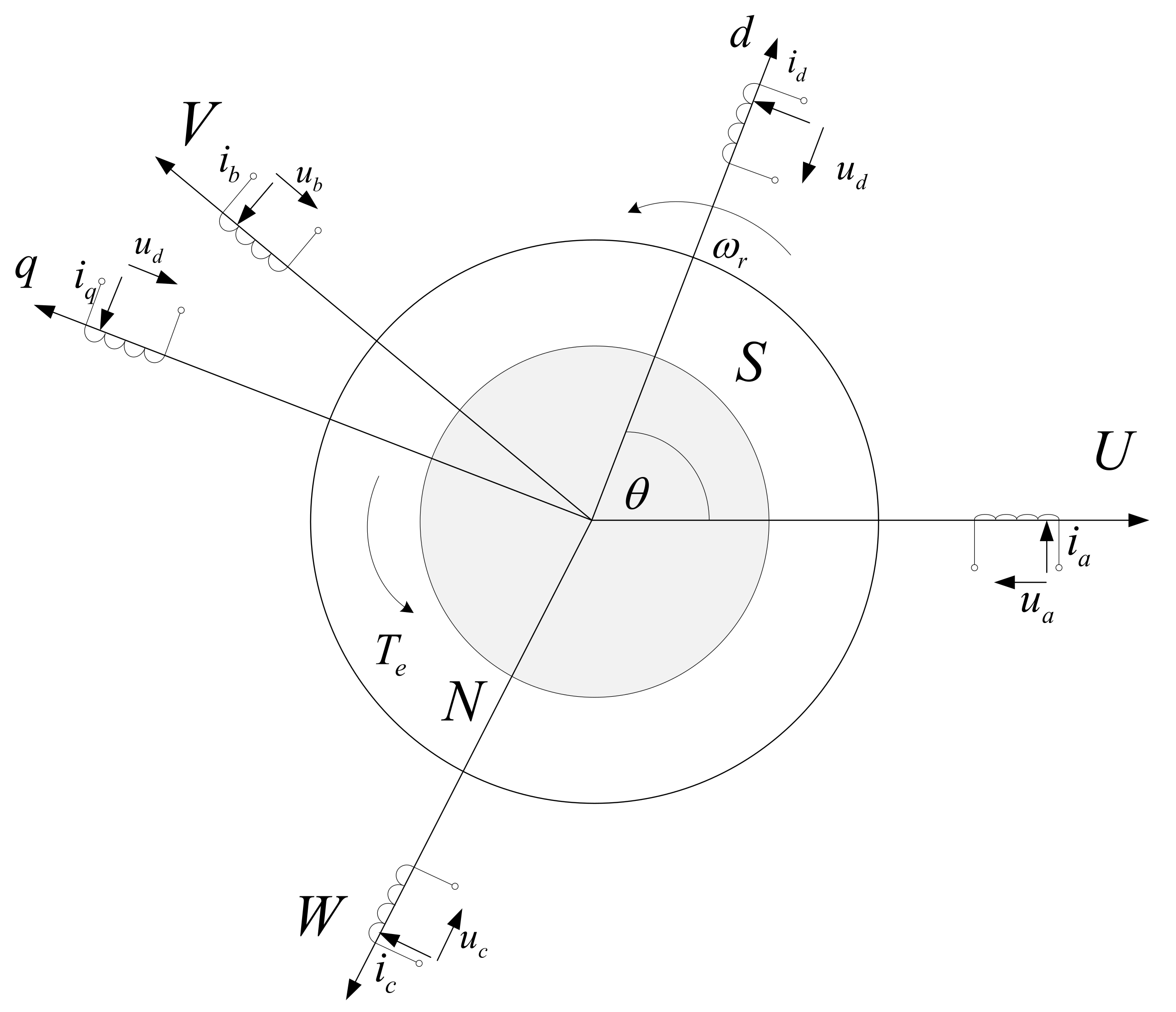
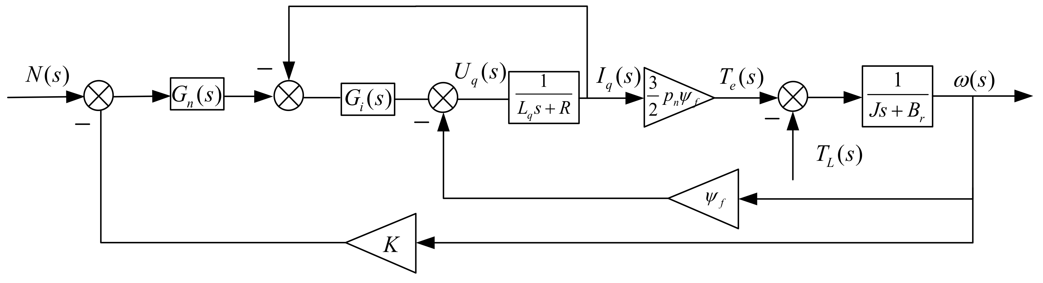
2.2.1. The Mathematical Model of AC Servo Motor

The physical model of the surface-mounted AC servo motor [15] is shown in Figure 2.

In order to simplify the mathematical model, the static stator three-phase winding of the AC servo motor can be equivalent to the shaft two-phase winding, which rotates synchronously with the rotor and is relatively static. At the same time, ignore the influence of the shaft voltage component of coordinate axis $q$, and the simplified voltage formula is shown as follows:

$$\left\{\begin{array}{l}{u}_d=R{i}_d+L_d\frac{\mathrm{d}}{\mathrm{d}t}{i}_d-{\omega }_e{L}_q{i}_q\hfill \\ u_q=R{i}_q+L_q\frac{\mathrm{d}}{\mathrm{d}t}{i}_q+{\omega }_e{\psi }_f\hfill \end{array}\right.$$

(1)

where, $u_d$ is the $d$-axis component of stator voltage; $u_q$ is the $q$-axis component of stator voltage; $i_d$ is $d$-axis components of stator current, $L_d$ is the stator $d$-axis equivalent inductance; $L_q$ is the stator $q$-axis equivalent inductance, $i_q$ is $q$-axis components of the stator current, ${\omega }_e$ is the electrical angular velocity, and $R$ is the equivalent resistance of stator winding.

The AC servo motor selected in this paper is a surface-mounted three-phase synchronous motor, so the equivalent values of the inductance of the stator winding are equal in the $d-q$ axis. So, the electromagnetic torque formula is shown as follows:

$$T_e=\frac{3}{2}{p}_n{i}_q{\psi }_f$$

(2)

where $T_e$ is the electromagnetic torque and the $p_n$ is the number of magnetic poles of motor.

Laplace transform of Formulas (1) and (2) is shown below.

$$\left\{\begin{array}{c}\begin{array}{l}\omega (s)=\frac{1}{Js+B_r}[T_e(s)-T_L(s)]\\ T_e(s)=\frac{3}{2}{p}_n{\psi }_f{I}_q(s)\end{array}\hfill \\ I_q(s)=\frac{U_q(s)-{\psi }_f\omega (s)}{L_{q}s+R}\hfill \end{array}\right.$$

(3)

Let $G_n(s)=k_{np}+\frac{k_{ni}}{s}$ and $G_i(s)=k_{ip}+\frac{k_{ii}}{s}$ denote the PI controller of the motor speed loop and current loop.

The transmission control block diagram of the AC servo motor is obtained, as shown in Figure 3.

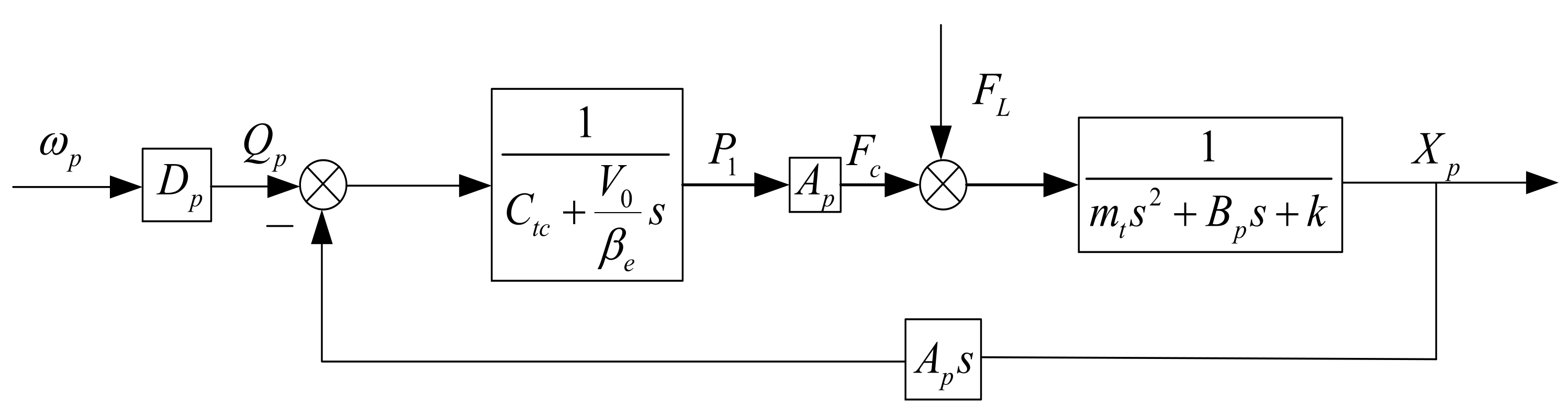
2.2.2. The Mathematical Model of the Pump-Controlled Cylinder System

The hydraulic pump studied in this paper is an inclined plate axial piston pump [16,17,18]. Assuming that at a certain time, the number of pistons at the hydraulic position is $n$, then the instantaneous flow of the piston pump is shown as follows:

$$\begin{array}{l}Q=Q_1+Q_2+\dots +Q_n={\displaystyle \sum _{i=1}^n{Q}_1}\\ =AR\omega \tan \gamma {\displaystyle \sum _{i=1}^n\sin {\psi }_i}\end{array}$$

(4)

where $A$ is the cross-sectional area of the plunger, $R$ is the single piston radius, and $w$ is the single plunger angular velocity.

It can be seen from Formula (4) that the axial velocity of the piston of the swashplate piston pump changes according to the sine law, and the flow discharged by multiple pistons will superimpose a relatively uniform flow. Therefore, the displacement formula of the piston pump can be shown as follows:

$$V=\frac{\pi d^2}{2}zR\tan \gamma .$$

(5)

The output flow of the variable pump is shown as follows:

$$q_p=V{\omega }_p-C_p(p_1-p_2)$$

(6)

where $V$ is the displacement of the piston pump, $d$ is the piston diameter, $z$ is the number of plungers, $R$ is the distribution circle radius of each plunger, $\gamma$ is the swash plate angle, and $C_p$ is the Leakage coefficient of piston pump.

The flow continuity formulas of the hydraulic cylinder are established below. The continuous flow formula of a rodless cavity is shown as follows:

$$q_1=A_1\frac{\mathrm{d}{x}_p}{\mathrm{d}t}+C_{i\mathrm{c}}(p_1-p_2)+C_{ec}{p}_1+\frac{V_{01}}{{\beta }_e}\frac{\mathrm{d}{p}_1}{\mathrm{d}t}.$$

(7)

The continuous formula of rod cavity flow is shown as follows:

$$q_2=-A_2\frac{\mathrm{d}{x}_p}{\mathrm{d}t}+C_{i\mathrm{c}}(p_1-p_2)-C_{ec}{p}_1-\frac{V_{02}}{{\beta }_e}\frac{\mathrm{d}{p}_2}{\mathrm{d}t}.$$

(8)

It is assumed that the initial volumes of the two cavities are equal, that is $V_t=V_{01}=V_{02}$, the average flow is taken as the load flow.

$$q_{\mathrm{L}}=\frac{\left(q_1+q_2\right)}{2}$$

(9)

$$q_L=\frac{\left(A_1+A_2\right)}{2}\frac{{\mathrm{dx}}_p}{\mathrm{d}t}+\frac{V_0}{{\beta }_{\mathrm{e}}}\left(\frac{\mathrm{d}{p}_1}{\mathrm{d}t}-\frac{\mathrm{d}{p}_2}{\mathrm{d}t}\right)+\left(\frac{C_{ec}}{2}+C_{ic}\right)p_L$$

(10)

where $C_{i\mathrm{c}}$ is the leakage coefficient in the hydraulic cylinder, $C_{ec}$ is the leakage coefficient outside the hydraulic cylinder, $A_1$ is the cross-sectional area of the rodless cavity piston rod in the hydraulic cylinder, $A_2$ is the hydraulic cylinder rod cavity piston rod cross-sectional area, $V_{01}$ is the initial volume of the rodless cavity of the hydraulic cylinder, $V_{02}$ is the initial volume of the hydraulic cylinder with the rod cavity, $q_{\mathrm{L}}$ is the load flow, $q_1$ is the rodless cavity flow, $q_2$ is the rod cavity flow, and ${\beta }_e$ is the effective bulk modulus.

According to Newton’s second law, the formula of balancing forces for the hydraulic cylinder and load is shown as follows:

$$F_c=A_p(p_1-p_2)=m_t\frac{d^2{x}_p}{dt}+B_p\frac{d{x}_p}{dt}+k{x}_p+F_L$$

(11)

where $m_t$ is the total mass of the piston and load converted to piston, $B_p$ is the viscous damping coefficient, $k$ is the load spring stiffness, $F_L$ is the load force, $C_{tc}$ is the total leakage coefficient, and $A_p$ is the effective area of hydraulic cylinder at work.

Laplace transform of the above formula has the following transfer function:

$$\left\{\begin{array}{l}{Q}_p(s)=D_p{\omega }_p(s)-C_{tp}{P}_1(s)\\ Q_p(s)=C_{tc}{P}_1(s)+A_p{X}_p(s)+\frac{V_0}{{\beta }_e}s{P}_1(s)\\ F_g(s)=A_p{P}_1(s)=m_t{s}^2{X}_p(s)+B_{p}s{X}_p(s)+k{X}_p(s)+F_L(s)\end{array}\right..$$

(12)

According to the above formulas, the pump-controlled cylinder transfer block diagram is shown in Figure 4.

In summary, the PCHPS transfer block diagram is shown in Figure 5.

3. Adaptive Integration Robust Control Algorithm

3.1. Adaptive Integration Robust Controller

3.1.1. System State Space Expression

In order to make the designed controller simple and stable, the transfer function of the AC servo motor is simplified as a proportional link, and its dynamic characteristics and unmodeled parts can be compensated by robust control. According to the mathematical model of the PCHPS, the status variables are selected as follows:

$$x={\left[x_1,x_2,x_3\right]}^T\triangleq {\left[y,\dot{y},A_1{P}_1/m_t-A_2{P}_2/m_t\right]}^T.$$

(13)

The state-space expression of the PCHPS is shown as follows:

$$\begin{array}{l}{\dot{x}}_1=x_2\hfill \\ {\dot{x}}_2=x_3-b{x}_2+f_0+d\left(t,x_1,x_2\right)\hfill \\ {\dot{x}}_3={\theta }_1{f}_{1}u-{\theta }_2{f}_2-{\theta }_3{f}_3\hfill \end{array}$$

(14)

where ${\theta }_1=D_p{}_e{\beta }_e$, ${\theta }_2={\beta }_e$, and ${\theta }_3=C_i{\beta }_e$, which makes $f_0=\frac{f}{m_t}({\sigma }_{0}z+{\sigma }_1\dot{z}+{\sigma }_{2}v)$, $f_1=\frac{1}{m_t}\left(\frac{A_1}{V_1}+\frac{A_2}{V_2}\right)$, $f_2=\frac{1}{m_t}\left(\frac{A_1{}^2}{V_1}+\frac{A_2{}^2}{V_2}\right)x_2$, $f_3=\frac{P_L}{m_t}\left(\frac{A_1}{V_1}+\frac{A_2}{V_2}\right)$, and $b=\frac{B}{m_t}$, in which $C_i$ is the leakage coefficient of the hydraulic cylinder, $d\left(t,x_1,x_2\right)$ is the centralized nominal function of system unmodeled dynamics, and $D_p{}_e$ is the equivalent displacement.

For the unknown parameter $\theta$, assume that the parameter is bounded and satisfied

$$\theta \in {\mathsf{\Omega }}_{\theta }=\left\{\theta :{\theta }_{\min }\le \theta \le {\theta }_{\max }\right\}$$

(15)

where ${\theta }_{\min }=[{\theta }_{1\min },{\theta }_{2\min },{\theta }_{3\min }]$, ${\theta }_{\max }=[{\theta }_{1\max },{\theta }_{2\max },{\theta }_{3\max }]$, and ${\theta }_{\min }$ and ${\theta }_{\max }$ are known. $d\left(t,x_1,x_2\right)$ is considered smooth enough to be satisfying

$$\left|\dot{d}\right|\le {\delta }_1\left|\ddot{d}\right|\le {\delta }_2.$$

3.1.2. Controller Design

Firstly, based on the definition of the projective function, the parameter adaptive law is designed; let $\widehat{\theta }$ denote the estimate of unknown parameters $\theta$, $\tilde{\theta }$ representing the estimation error of unknown parameter vectors $\theta$, that is, $\tilde{\theta }=\widehat{\theta }-\theta$, which is shown as follows:

$$\dot{\widehat{\theta }}=Pro{j}_{\widehat{\theta }}(\mathsf{\Gamma }\tau )$$

where $\mathsf{\Gamma }$ is the parameter adaptive rate diagonal matrix, and $Pro{j}_{\widehat{\theta }}$ is a discontinuous insinuation function, which can be shown as follows:

$${\mathrm{Proj}}_{{\widehat{\theta }}_i}\left({\tau }_i\right)=\left\{\begin{array}{cc}0,\hfill & \mathrm{if}{\widehat{\theta }}_i={\theta }_{i\max }\mathrm{and}{\tau }_i>0\hfill \\ 0,\hfill & \mathrm{if}{\widehat{\theta }}_i={\theta }_{i\min }\mathrm{and}{\tau }_i<0\hfill \\ {\tau }_i,\hfill & \mathrm{otherwise}\hfill \end{array}\right..$$

(16)

For arbitrary $\tau$, the projective function satisfies the following two properties

$$\begin{array}{l}1.\widehat{\theta }\in {\mathsf{\Omega }}_{\widehat{\theta }}\triangleq \left\{\widehat{\theta }:{\theta }_{\min }\le \widehat{\theta }\le {\theta }_{\max }\right\}\\ 2.{\tilde{\theta }}^T\left[{\mathsf{\Gamma }}^{-1}{\mathrm{Proj}}_{\widehat{\theta }}(\mathsf{\Gamma }\tau )-\tau \right]\le 0,\forall \tau \end{array}$$

Since the system is not modeling dynamics and external interference exists, the controller is designed by an anti-stepping method. According to Formula (14), the first formula does not contain any uncertainty. Set $x_d$ to the input track, which defines the following error variables.

$$\begin{array}{l}{e}_1=x_1-x_d\\ e_2={\dot{e}}_1+k_1{e}_1=x_2-x_{2eq},x_{2eq}\triangleq {\dot{e}}_{1d}-k_1{e}_1\end{array}$$

(17)

where $e_1$ is the tracking error, $k_1$ is any positive feedback gain, the $G_{e1}(s)=\frac{e_1(s)}{e_2(s)}=\frac{1}{s+k_1}$ is the controller representing the error ring, wherein, when $e_1$ becomes small enough or converges to zero, $e_2$ also becomes small enough or converges to zero. So, the following design goal is to make $e_2$ as small as possible while ensuring stable transient performance. Additional controller design freedom is obtained by designing auxiliary error signals $r$.

$$\begin{array}{ll}r& =x_3-{\dot{x}}_{2eq}+k_2{e}_2-b{x}_2+f_0+d\left(t,x_1,x_2\right)\\ & =e_3+{\alpha }_2-{\dot{x}}_{2eq}+k_2{e}_2-b{x}_2+f_0+d\left(t,x_1,x_2\right)\end{array}$$

(18)

where ${\alpha }_2$ is the virtual control law of the state variable $x_3$, and $e_3$ is the deviation between the two.

For virtual control law ${\alpha }_2$, its structure and expression are described as follows

$$\begin{array}{l}{\alpha }_2={\alpha }_{2a}+{\alpha }_{2s}\\ {\alpha }_{2a}={\dot{x}}_{2eq}-k_2{e}_2+b{x}_2-{\widehat{f}}_0\\ {\alpha }_{2s}={\alpha }_{2s1}+{\alpha }_{2s2},{\alpha }_{2s1}=-k_r{z}_2\end{array}$$

(19)

where ${\alpha }_{2a}$ is model-based feedback control law, and ${\alpha }_{2s}$ is the robust control part. The ${\alpha }_{2s1}$ is designed as a linear robust feedback control law, which is used to stabilize the nominal model of the hydraulic system.

The above formulas can be obtained:

$$r=e_3-k_r{e}_2+{\alpha }_{2s2}+d\left(t,x_1,x_2\right).$$

(20)

In order to overcome the effect of modeling uncertainty and unknown external interference on the system, the error symbol integral robust control item is introduced here. Therefore, ${\alpha }_{2s2}$ can be expressed as follows:

$${\alpha }_{2s2}=-{\displaystyle {\int }_0^t{k}_r}{k}_2{e}_2+\beta \mathrm{sign}\left(e_2\right)d\nu$$

(21)

where $\beta$ is the integral robust feedback gain; $\mathrm{sign}\left(e_2\right)$ is a standard symbol function about errors $e_2$.

In order to obtain the actual control input of the system, the following face (20) is guided

$$\begin{array}{ll}\dot{r}& ={\dot{z}}_3-k_r{\dot{z}}_2+{\dot{\alpha }}_{2s2}+\dot{d}\\ & ={\dot{x}}_3-{\dot{\alpha }}_2-k_{r}r-\beta \mathrm{sign}\left(z_2\right)+\dot{d}\end{array}$$

(22)

The joint Formulas (20) and (22) are available

$$\dot{r}={\theta }_1{f}_{1}u-{\theta }_2{f}_2-{\theta }_3{f}_3-{\dot{\alpha }}_2-k_{r}r-\beta \mathrm{sign}\left(z_2\right)+\dot{d}.$$

Due to the uncertainty of parameters, the actual input of the system consists of estimates of unknown parameters.

$$\begin{array}{l}u=u_a+u_s\\ u_a=\frac{{\widehat{\theta }}_2{f}_2+{\widehat{\theta }}_3{f}_3+{\dot{\alpha }}_2}{{\widehat{\theta }}_1{f}_1}\\ u_s=\frac{-k_3{z}_3}{f_1}\end{array}$$

(23)

In the upper, $k_3$ is the positive feedback gain, $u_a$ is an adjustable model compensation control by updating parameters online, and $u_s$ is a robust control. So, Formulas (22) and (23) are available,

$$\dot{r}=-{\phi }^T\tilde{\theta }-k_3{\theta }_1{e}_3-k_{r}r-\beta \mathrm{sign}\left(e_2\right)+\dot{d}$$

(24)

$$\phi ={\left[f_1{u}_a,-f_2,-f_3\right]}^T.$$

$\phi$ is the regression vector of the parameter adaptation, and the $e_3$’s dynamic characteristics are shown as follows:

$${\dot{e}}_3=-{\phi }^T\tilde{\theta }-k_3{\theta }_1{e}_3.$$

(25)

The performance of the controller is analyzed below.

Define the auxiliary function $L(t)=r\left[\dot{d}-\beta \mathrm{sign}\left(e_2\right)\right]$. When the robust gain $\beta$ satisfies the inequality $\beta \ge {\delta }_1+\frac{1}{k_2}{\delta }_2$, the auxiliary function $P(t)=\beta \left|e_2(0)\right|-e_2(0)\dot{d}(0)-{\displaystyle {\int }_0^{t}L}(\nu )d\nu$ is constantly positive. The adaptive function selected by the controller is $\tau =\phi \left(r+e_3\right)$.

Define the feedback gain matrix $\mathsf{\Lambda }$, and the value of the feedback gain $k_1,k_2,k_3,k_r$ is large enough to make the gain matrix $\mathsf{\Lambda }$ a positive matrix.

$$\mathsf{\Lambda }=\left[\begin{array}{cccc}{k}_1& -1/2& 0& 0\\ -1/2& k_2& -1/2& 0\\ 0& -1/2& k_r& {\theta }_1{k}_3/2\\ 0& 0& {\theta }_1{k}_3/2& {\theta }_1{k}_3\end{array}\right]$$

(26)

Select the Lyapunov function $V=\frac{1}{2}\left(e^{T}e+{\tilde{\theta }}^T{\mathsf{\Gamma }}^{-1}\tilde{\theta }\right)+P(t)$; therefore,

$$\dot{V}=-e^T\mathsf{\Lambda }e+{\tilde{\theta }}^T{\mathsf{\Gamma }}^{-1}(\dot{\widehat{\theta }}-\mathsf{\Gamma }\tau ).$$

(27)

Depending on the nature of the innuendo function, it can be seen that $\dot{V}\le -e^T\mathsf{\Lambda }e$; since the gain matrix $\mathsf{\Lambda }$ is a positive matrix, there is

$$\dot{V}\le -{\lambda }_{\min }(\mathsf{\Lambda })\left(e_1^2+e_2^2+r^2+e_3^2\right)\triangleq -W$$

(28)

$-{\lambda }_{\min }(\mathsf{\Lambda })$ is the minimum characteristic value of the gain matrix.

Then, when the numerical selection of the relevant control parameters meets the above conditions, all the signals of the system are bounded under closed-loop control, and the control system also obtains the progressive output tracking performance of the signal, that is, when $t\to \infty$, $e_1\to 0$.

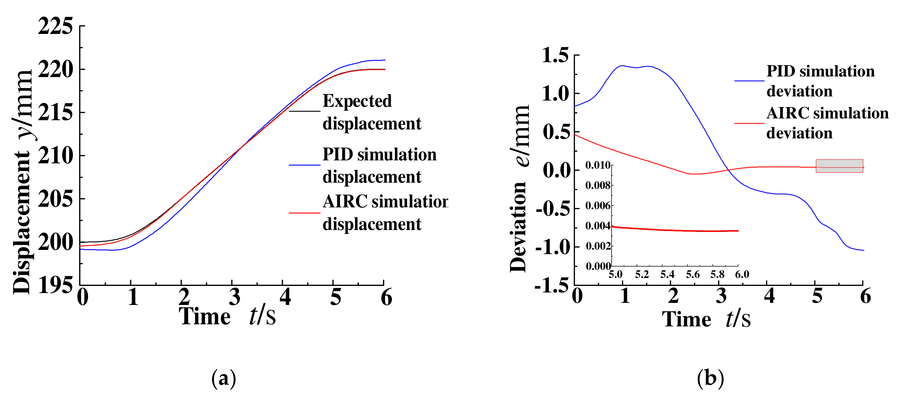
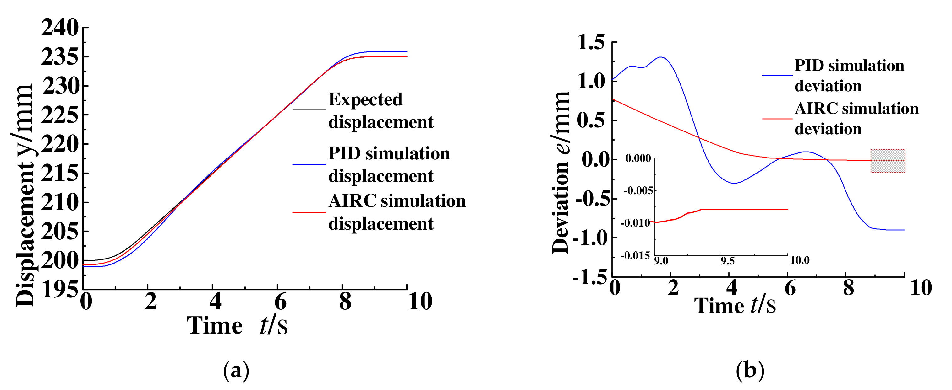
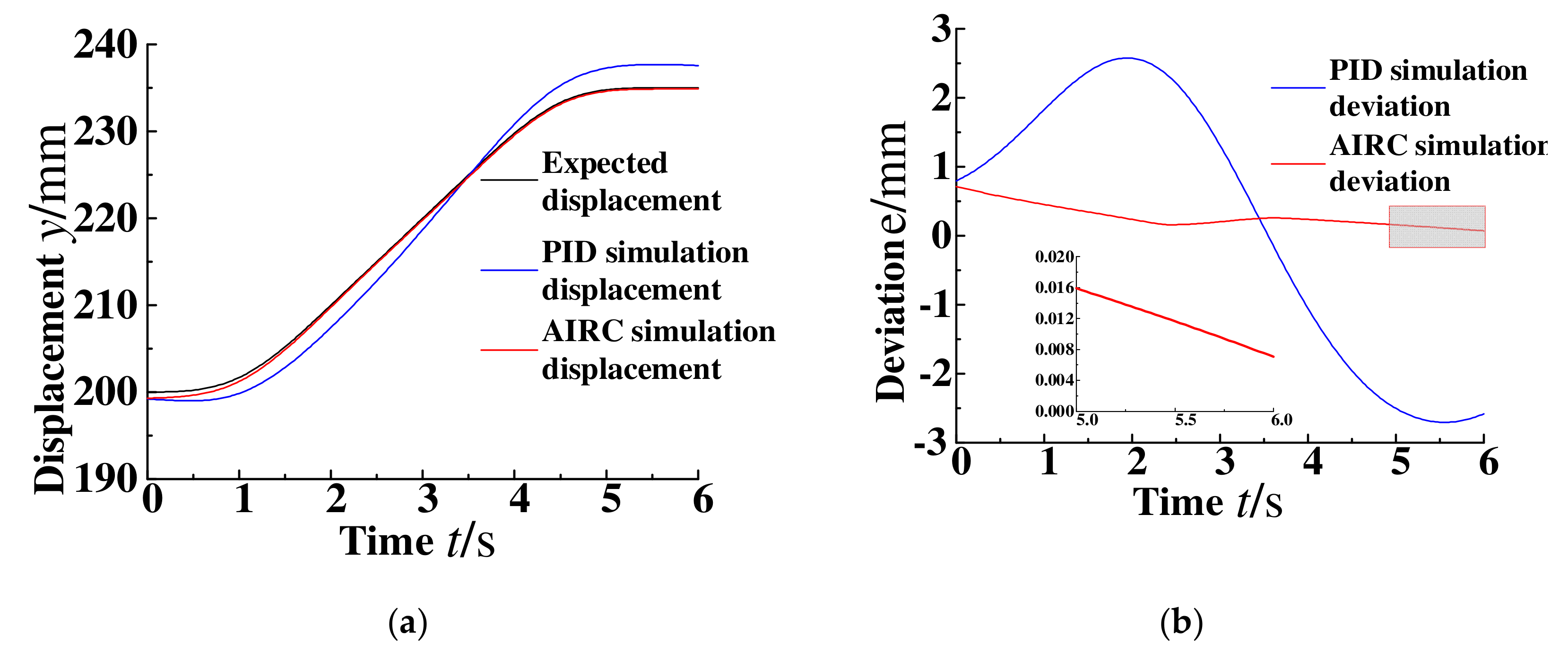
3.2. The Dynamic Simulation of PCHPS

In this section, the adaptive integral robust control algorithm designed above is verified by MATLAB/Simulink simulation platform, At the same time, the dead zone and some nonlinear disturbances are added to the PCHPS to make the system simulation characteristics closer to the reality. The values of relevant control parameters of an adaptive integral robust controller are as follows.

$k_1=1200,k_2=200,k_3=50,k_r=300$	—	Controller gain;
${\widehat{\theta }}_1\left(0\right)=26990,{\widehat{\theta }}_2\left(0\right)=1.24\times {10}^9,{\widehat{\theta }}_3\left(0\right)=0.005$	—	The initial values of the adaptive parameters;
$\mathsf{\Gamma }=diag\left\{6\times {10}^{-5},1.8\times {10}^9,1\times {10}^{-10}\right\}$	—	Parameter adaptive gain;
$\beta =300$	—	Robust control gain.

The track planning table for verifying the AIRC is shown in

Table 1. Motion track planning table.

Conditions	Acceleration (mm/s3)	Max Acceleration (mm/s2)	Max Speed (mm/s)	Travel (mm)
①	5	5	5	20
②	5	5	5	35
③	5	5	10	35
④	10	10	10	35

.

Figure 6, Figure 7, Figure 8 and Figure 9 are the performance of the slow motion phase of the PCHPS from simulation operating conditions (1) to (4).

It can be seen from Figure 6, Figure 7, Figure 8 and Figure 9 that after adding a dead zone and nonlinear interference to the simulation model, the tracking performance and positioning accuracy of the PCHPS under the PID algorithm cannot show an ideal control performance. When the position control algorithm of the system is changed to the AIRC algorithm, the motion trajectory of the system overcomes the original lag in a short time, and it starts to track the planned trajectory of the system stably, with the deviation kept within the range of 0 to 0.2 mm. When the system runs to the specified position, there is almost no over range, and the positioning accuracy is within 0.005 mm; thus, the control effect is very ideal. The simulation results show that the designed AIRC algorithm greatly improves the positioning accuracy and improves the position control performance of the PCHPS.

4. Experimental Verification of PCHPS

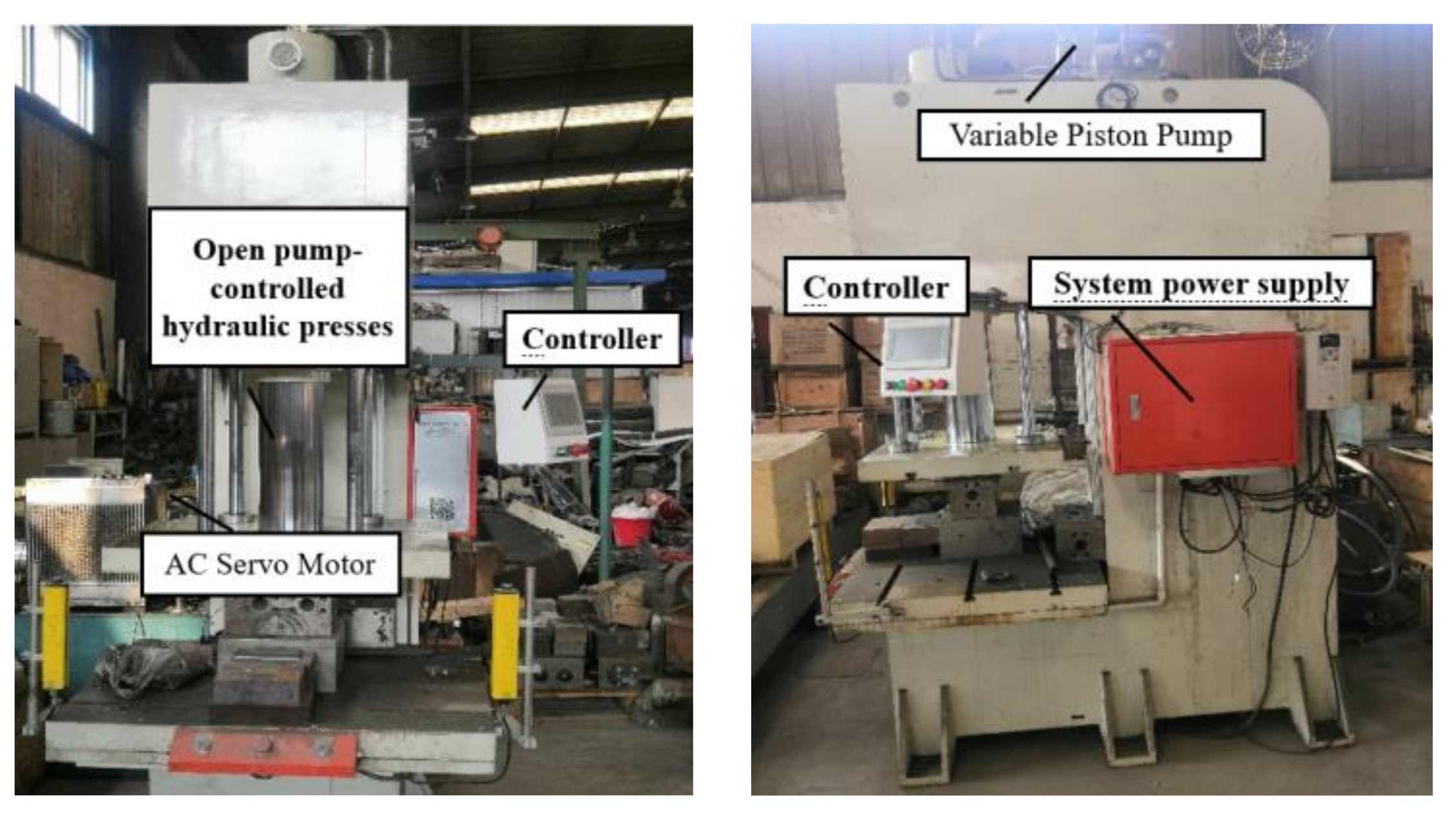
4.1. Experimental Test Platform of PCHPS

In order to verify the effectiveness of the friction compensation and control algorithm of the open PCHPS, Figure 10 is an industrial open PCHPS made of a Figure 1 schematic.

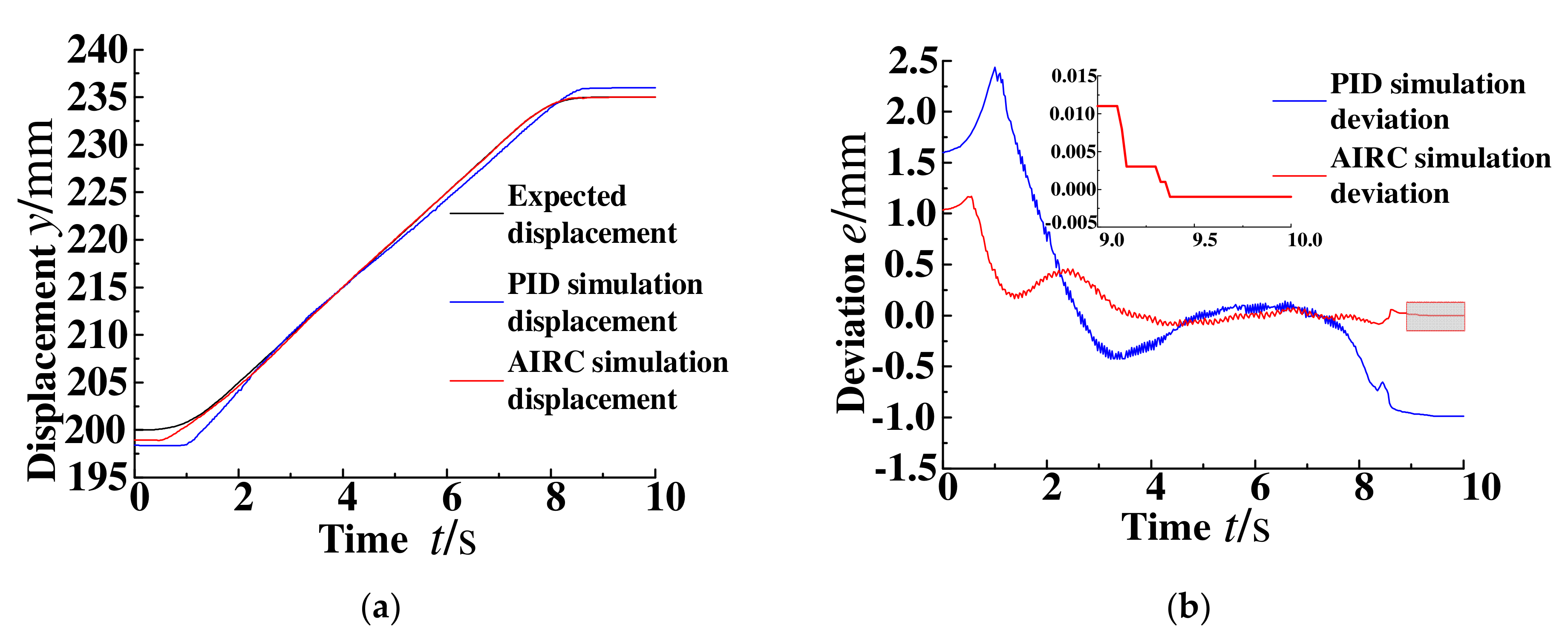
4.2. Experimental Test of PCHPS

The slow-down stage of the system is running at a low speed and is very susceptible to unknown interference from the system and the outside, so the motion stage uses an AIRC controller with the same controller parameter settings as the 3.2 simulation parameters; see Figure 11, Figure 12, Figure 13 and Figure 14. The figure shows the position control performance of the system after adjustment with the conventional PID algorithm after adjusting the AIRC algorithm.

It can be seen that in the initial stage of slow-down motion of the hydraulic cylinder, the phenomenon in which the actual displacement is ahead of the expected displacement after a period of motion has been greatly improved. The actual displacement curve of the system does not change greatly after gradually approaching the trajectory curve of the motion planning, showing good position tracking performance and fully overcoming the positioning error in the fast-down stage. Through the displacement deviation curves under various working conditions, it can be found that the variation of system deviation under the AIRC algorithm is gentler than that under the PID algorithm, and the deviation values are significantly smaller than those under the PID algorithm. When the system moves slowly to the deceleration stage of the planned trajectory, the deviation of the system gradually approaches zero. This can fully ensure that the system avoids the occurrence of over-range phenomenon to the greatest extent, the final positioning accuracy is significantly improved, and the difference is finally stabilized at about $\pm$0.005 mm. It can be seen that the AIRC algorithm fully overcomes the negative impact of unknown disturbances and parameter changes in the slow stage of the system, and it gives the appropriate control compensation for the system position.

5. Discussion

5.1. The Research Background and Significance of Hydraulic Press

The pump-controlled hydraulic presses adopts the volume control mode. Compared with the valve-controlled hydraulic system, the heating of the pump-controlled hydraulic system is reduced and the energy utilization rate can be increased by more than 40%. In addition, the pump-controlled system has a compact structure and is convenient for installation and maintenance. The nonlinear factors of hydraulic system affect and restrict the control accuracy and quality of the system to a great extent. The traditional linearization control strategy cannot cover and deal with these nonlinear factors, and its limitations can be seen here. Therefore, it is of great research value to deal with the nonlinear factors in the pump-controlled system and design the nonlinear control method to improve the control performance of the system.

According to the system characteristics of a pump-controlled hydraulic press, this paper designs a reasonable nonlinear control method and tries to compensate for the nonlinear friction phenomenon in the system, in order to obtain a higher precision system control performance and lay a good theoretical research foundation for improving the control performance of PCHPS.

5.2. The Selection of Control Strategy

There are many nonlinear links and links that cannot establish an accurate model in the PCHPS. In many studies, nonlinear control methods are introduced into the compensation control of nonlinear factors of an electro-hydraulic servo system in order to obtain a better control effect. Bin Yao of Purdue University proposed a general adaptive robust controller design method. The robust control part is used to reduce the influence of the unknown modeling part on system stability [19,20], and the parameter adaptation is used to reduce the uncertainty of model parameters. Bin Yao has carried out a detailed mathematical derivation and demonstration on the controller structure and proved that the controller can overcome nonlinear factors and be asymptotically stable.

It is proved by investigation and actual situation that the adaptive integral robust control method can obviously suppress the interference in the system. Especially for the unmodeled part of the mathematical model, there is inaccuracy in the parameters and uncertain external interference in the modeled part. The method used in this study can reduce the adverse impact of the above interference on the system.

6. Conclusions

In this paper, PCHPS is taken as the research object. Through simulation and experimental comparison, the position control performance of the system in the fast and slow motion stages of the conventional control algorithm is analyzed. The control algorithms are designed for the main factors affecting the position control accuracy in each motion stage, and the position compensation control of the pump-controlled hydraulic press is analyzed. The mathematical mechanism models of a permanent magnet synchronous AC servo motor and pump-controlled cylinder are established respectively, and the simulation model of a PCHPS machine is built by MATLAB/Simulink software. An AIRC algorithm for the PCHPS is proposed to compensate for the unknown interference, parameter variation, and model inaccuracy in the system. Simulation and experiments show that the AIRC algorithm can effectively overcome the nonlinear interference of the system, improve the position control effect of the system, and greatly improve the positioning accuracy of the hydraulic press.

References

1. Yan, X.; Chen, B. Analysis of a novel energy-efficient system with 3-D vertical structure for hydraulic press. Energy 2020, 218, 119518. [Google Scholar] [CrossRef]
2. Huang, H.; Zou, X.; Li, L.; Li, X.; Liu, Z. Energy-Saving Design Method for Hydraulic Press Drive System with Multi Motor-Pumps. Int. J. Precis. Eng. Manuf.-Green Technol. 2019, 6, 223–234. [Google Scholar] [CrossRef]
3. Feng, J.; Yu, B.; Li, X.; Yao, J.; Kong, X.; Guo, H. Study of ADRC on fluid power transmission system control characteristics of 60MN hydraulic press. In Proceedings of the 2015 International Conference on Fluid Power and Mechatronics (FPM), Harbin, China, 5–7 August 2015; pp. 660–666. [Google Scholar] [CrossRef]
4. Ba, K.; Song, Y.; Shi, Y.; Wang, C.; Ma, G.; Wang, Y.; Yu, B.; Yuan, L. A Novel One-Dimensional Force Sensor Calibration Method to Improve the Contact Force Solution Accuracy for Legged Robot. Mech. Mach. Theory 2022, 169, 104685. [Google Scholar] [CrossRef]
5. Li, J.; You, B.; Ding, L.; Yu, X.; Li, W.; Zhang, T.; Gao, H. Dual-Master/Single-Slave Haptic Teleoperation System for Semiautonomous Bilateral Control of Hexapod Robot Subject to Deformable Rough Terrain. IEEE Trans. Syst. Man Cybern. Syst. 2021, 1–15. [Google Scholar] [CrossRef]
6. Ba, K.; Song, Y.; Yu, B.; Wang, C.; Li, H.; Zhang, J.; Ma, G. Kinematics correction algorithm for the LHDS of a legged robot with semi-cylindrical foot end based on V-DOF. Mech. Syst. Signal Processing 2022, 167, 108566. [Google Scholar] [CrossRef]
7. Yin, S.; Yang, H.; Xu, K.; Zhu, C.; Wang, Y. Location of abnormal energy consumption and optimization of energy efficiency of hydraulic press considering uncertainty. J. Clean. Prod. 2021, 294, 126213. [Google Scholar] [CrossRef]
8. Xuan, W.; Fanquan, Z. Design of electro-hydraulic servo loading controlling system based on fuzzy intelligent water drop fusion algorithm. Comput. Electr. Eng. 2018, 71, 485–491. [Google Scholar] [CrossRef]
9. Macchelli, A.; Barchi, D.; Marconi, L.; Bosi, G. Robust Adaptive Control of a Hydraulic Press. IFAC-PapersOnLine 2020, 53, 8790–8795. [Google Scholar] [CrossRef]
10. Jin, X.; Chen, K.; Zhao, Y.; Ji, J.; Jing, P. Simulation of hydraulic transplanting robot control system based on fuzzy PID controller. Measurement 2020, 164, 108023. [Google Scholar] [CrossRef]
11. Liu, D.; Li, C.; Malik, O.P. Nonlinear modeling and multi-scale damping characteristics of hydro-turbine regulation systems under complex variable hydraulic and electrical network structures. Appl. Energy 2021, 293, 116949. [Google Scholar] [CrossRef]
12. Maier, C.C.; Schröders, S.; Ebner, W.; Köster, M.; Fidlin, A.; Hametner, C. Modeling and nonlinear parameter identification for hydraulic servo-systems with switching properties. Mechatronics 2019, 61, 83–95. [Google Scholar] [CrossRef]
13. Dang, X.; Zhao, X.; Dang, C.; Jiang, H.; Wu, X.; Zha, L. Incomplete differentiation-based improved adaptive backstepping integral sliding mode control for position control of hydraulic system. ISA Trans. 2020. prepublish. [Google Scholar] [CrossRef] [PubMed]
14. Soon, C.C.; Ghazali, R.; Jaafar, H.I.; Hussien, S.Y.S. Sliding Mode Controller Design with Optimized PID Sliding Surface Using Particle Swarm Algorithm. Procedia Comput. Sci. 2017, 105, 235–239. [Google Scholar] [CrossRef]
15. Borisov, O.I.; Pyrkin, A.A.; Isidori, A. Robust Output Regulation of Permanent Magnet Synchronous Motors by Enhanced Extended Observe. IFAC-PapersOnLine 2020, 53, 4881–4886. [Google Scholar] [CrossRef]
16. Pang, H.; Wu, D.; Deng, Y.; Cheng, Q.; Liu, Y. Effect of working medium on the noise and vibration characteristics of water hydraulic axial piston pump. Appl. Acoust. 2021, 183, 108277. [Google Scholar] [CrossRef]
17. Bedotti, A.; Pastori, M.; Scolari, F.; Casoli, P. Dynamic modelling of the swash plate of a hydraulic axial piston pump for condition monitoring applications. Energy Procedia 2018, 148, 266–273. [Google Scholar] [CrossRef]
18. Babikir, H.A.; Abd Elaziz, M.; Elsheikh, A.H.; Showaib, E.A.; Elhadary, M.; Wu, D.; Liu, Y. Noise prediction of axial piston pump based on different valve materials using a modified artificial neural network model. Alex. Eng. J. 2019, 58, 1077–1087. [Google Scholar] [CrossRef]
19. Yao, B.; Bu, F.; Reedy, J.; Chiu, G.C. Adaptive robust motion control of single-rod hydraulic actuators: Theory and experiments. IEEE/ASME Trans. Mechatron. 2002, 5, 79–91. [Google Scholar]
20. Yao, B.; Bu, F.; Chiu, T.C. Nonlinear adaptive robust control of electro-hydraulic servo systems with discontinuous projections. In Proceedings of the IEEE Conference on Decision & Control, Tampa, FL, USA, 16–18 December 1998. [Google Scholar]
Figure 1. The principle of PCHPS.
Processes 10 00014 g001
Figure 2. AC servo motor physical model of SPMSM in a plane coordinate system.
Processes 10 00014 g002
Figure 3. Diagram of AC servo motor.
Processes 10 00014 g003
Figure 4. Pump-controlled cylinder transfer block diagram.
Processes 10 00014 g004
Figure 5. Electro-hydraulic servo position control system of PCHPS.
Processes 10 00014 g005
Figure 6. System displacement and deviation curve under working condition ①. (a) System displacement curve. (b) System displacement deviation curve.
Processes 10 00014 g006
Figure 7. System displacement and deviation curve under working condition ②. (a) System displacement curve. (b) System displacement deviation curve.
Processes 10 00014 g007
Figure 8. System displacement and deviation curve under working condition ③. (a) System displacement curve. (b) System displacement deviation curve.
Processes 10 00014 g008
Figure 9. System displacement and deviation curve under working condition ④. (a) System displacement curve. (b) System displacement deviation curve.
Processes 10 00014 g009
Figure 10. Open pump-controlled hydraulic electromechanical fluid servo position control system.
Processes 10 00014 g010
Figure 11. System displacement and deviation curve under working condition ①. (a) System displacement curve. (b) System displacement deviation curve.
Processes 10 00014 g011
Figure 12. System displacement and deviation curve under working condition ②. (a) System displacement curve. (b) System displacement deviation curve.
Processes 10 00014 g012
Figure 13. System displacement and deviation curve under working condition ③. (a) System displacement curve. (b) System displacement deviation curve.
Processes 10 00014 g013
Figure 14. System displacement and deviation curve under working condition ④. (a) System displacement curve. (b) System displacement deviation curve.
Processes 10 00014 g014