Abstract
This paper presents computational fluid dynamics (CFD) simulations of the flow around a horizontal axis hydrokinetic turbine (HAHT) found in the literature. The volume of fluid (VOF) model implemented in a commercial CFD package (ANSYS-Fluent) is used to track the air-water interface. The URANS SST k- and the four-equation Transition SST turbulence models are employed to compute the unsteady three-dimensional flow field. The sliding mesh technique is used to rotate the subdomain that includes the turbine rotor. The effect of grid resolution, time-step size, and turbulence model on the computed performance coefficients is analyzed in detail, and the results are compared against experimental data at various tip speed ratios (TSRs). Simulation results at the analyzed rotor immersions confirm that the power and thrust coefficients decrease when the rotor is closer to the free surface. The combined effect of rotor and support structure on the free surface evolution and downstream velocities is also studied. The results show that a maximum velocity deficit is found in the near wake region above the rotor centerline. A slow wake recovery is also observed at the shallow rotor immersion due to the free-surface proximity, which in turn reduces the power extraction.
1. Introduction
Hydraulic energy sources around the world are primarily used on large hydroelectric plants which provide electricity to densely populated areas. Colombia is rich in water resources with large hydropower schemes covering roughly 79% of the energy generation (54,532 GWh, data of 2019), while the remaining 21% mainly comes from coal and gas sources which both come at a high environmental cost [1]. The hydropower schemes are generally conventional hydroelectric dams which use a reservoir and dam set-up, and also run-of-the-river hydroelectricity which have no reservoir, similar to the world-renowned Hoover dam on the border between the states of Nevada and Arizona, USA [2]. The construction of conventional hydropower schemes poses a risk to the environment and nearby communities. The under-construction 2.4 GW Ituango hydroelectric project will be the largest hydropower plant in Colombia. One of Ituango’s auxiliary diversion tunnels collapsed in 2018; the water had to be diverted to prevent the overflow of the dam and spillway. The resulting high-speed flow in the adduction tunnels produced rock instabilities that compromised the integrity of the whole structure [3]. The population of Colombia is expected to grow by 12% in 2050 [4], which will further increase the challenges in supplying sustainable renewable energy to the entire country and in reducing greenhouse gas emissions.
In Colombia, energy supply issues predominately affect isolated regions located away from the main electricity supply network. Alternative methods of energy generation from renewable resources offer a promising solution to tackle social inequality as well as reducing environmental impacts, such as air and water pollution and climate change due to the carbon emissions, and they would also reduce the local dependency on fossil fuels. The full potential of all types of renewable resources needs to be fully explored and integrated with novel solutions, such as hydrokinetic turbines. This technology does not require the use of large areas of land, contrary to conventional hydropower, while also being a significantly cheaper alternative due to the portability of hydrokinetic turbines as single assembled units, which facilitates deployment and maintenance [5]. To date, horizontal axis turbines have been preferred for large rivers due to their mature development owing to the wind industry. However, these devices are restricted to high-velocity regions and deep waters which are not always available in a riverine environment. It is therefore necessary to study the effect of rotor depth on the overall performance of horizontal-axis hydrokinetic turbines (HAHT), both experimentally and computationally. The work presented in this paper investigates the free-surface-turbine-wake interaction using computational fluid dynamics (CFD).
The most common numerical approaches to predict the rotor performance of HAHTs are borrowed from wind energy engineering. The BEM (blade-element momentum) theory, also referred to as strip theory, combines the balance of linear and angular momentum with the aerodynamic forces exerted on a blade section. BEM theory requires the knowledge of aerodynamic coefficients and the calculations of the axial and angular induction factors at the blade section. This information is used to integrate the balance equations along the blade length to estimate the total power from the rotor at the specified angular and flow velocities [6,7]. BEM theory can be used to estimate the performance of a HAHT when the rotor is well submerged into the water, so the rotor and free surface interaction can be neglected. Batten et al. [8] compared BEM results of thrust and power coefficients at various tip-speed ratios (TSR) with the experimental data of a laboratory-scale horizontal axis tidal turbine tested in a cavitation tunnel. Simulation results showed good agreement for power coefficient in the TSR range from 3 to 7; BEM underpredicted the thrust coefficient for the analyzed pitch angles. Similarly, Danao et al. [9] performed calculations with the open-source blade element momentum solver Qblade; and a good agreement was found for the power coefficient.
The actuator disk method (ADM) and the actuator line method (ALM) are two novel simulation techniques commonly used to simulate horizontal axis wind turbine rotors. In the ADM, the rotor is substituted by a non-rotating disk with the same area swept by the blades. A body-force term in the disk region is defined to account for the extraction of fluid momentum by the rotor [10]. Contrary to ALM, ADM is not able to reproduce root and tip vortices. i.e. the actuator disk just accounts for large-scale effects on the flow. Silva dos Santos et al. [11] used the ADM implemented in the commercial CFD software ANSYS-Fluent to simulate the wake characteristics of a hydrokinetic farm on a portion of the Brazilian Amazon river. In ALM, the complex geometry of rotor blades is simplified to a set of rotating lines. Distributed point forces are defined along those lines (actuator lines) to iteratively compute the loadings using BEM and available airfoil data with submodels for dynamic stall situations [12,13]. Next, the forces are projected onto the computational domain to account for the effect of rotating blades on the flow field. ALM avoids the computation of the blade boundary layer and the implementation of rotating meshes. The ALM technique has been successfully used to estimate the rotor performance and the wake behind wind turbines [14]. ALM combined with LES (large-eddy simulation) was used by Baba-Ahmadi and Dong [15] to simulate the flow through a horizontal axis tidal stream turbine. Axial velocity and turbulence intensity profiles behind the turbine at the rotor axis height showed good agreement with experimental results, although the velocity deficit was slightly overpredicted in the far wake. This study did not consider free-surface effects, i.e., it was a single-phase flow computation.
The number of investigations seeking to clarify the effects of the free surface on HAHT performance and wake dynamics is still limited. A complete CFD model of HAHT must include a fully resolved blade geometry and the definition of a rotating region that encloses the rotor in the computational domain. Tracking the interface requires the use of a multiphase framework, which further increases the computational cost. Disregarding the free surface in a computational approach can lead to significant differences in the predicted turbine performance. For a Darrieus turbine, Hocine et al. [16] reported an increment of 42.4% in power output and a 26.6% higher thrust when the free surface was neglected.
Previous computational and experimental studies have shown a decrease in thrust and power output by bringing the turbine closer to the free surface. Bahaj et al. [17] experimentally reported a reduction in power and thrust of approximately 8.8% and 4.5%, respectively, by taking the rotor to a blade tip immersion from 0.55D to 0.19D (D is the rotor diameter). Yan et al. [18] implemented a computational free-surface flow framework, with a novel level-set re-distancing technique and sliding interface, to perform three-dimensional, time-dependent simulations of a horizontal-axis tidal turbine. A turbulence model was not incorporated in their numerical approach. Results of power of thrust coefficients suggested the existence of a minimum immersion depth for optimal turbine operation. Conversely, Kolekar et al. [19] reported an increase in the power coefficient by reducing the rotor immersion, indicating a favorable depth region for the performance near a 0.27D immersion of the blade tip; they also observed significant changes in the wake dynamics, especially at shallow immersions in which the wake becomes asymmetric. Nishi et al. [20] showed an unusual increase in performance of up to 2.8 times when implementing a multiphase approach (water-air), compared to single-phase flow results (water only); the turbine output from the multiphase flow simulation is approximately 5% higher than the experimental data. Bai et al. [21] used the immersed boundary method and free surface method implemented in an in-house CFD code to simulate the turbine rotor of Bahaj et al. [17]. The computed power coefficient lay below the experimental data; a finer grid was shown to reduce the discrepancy at the TSR for maximum power output. Adamski [22] reported the appearance of large ripples (deformations) on the free surface when the distance to the rotor is decreased; the vertical deformation is approximately twice as much when the blade tip immersion is reduced from 1D to 0.75D.
Rodriguez et al. [23] performed two-phase flow simulations of the HAHT rotor described in Bahaj et al. [17], for two blade tip immersions and three TSRs. The computational approach incorporated a transition four-equation turbulence model, the Volume of Fluid (VOF) method for interface tracking, and the sliding-mesh technique to account for blade rotation. There was a good qualitative agreement between the simulation results of torque and thrust coefficients and the experimental data taken from Bahaj et al., at the analyzed TSRs. Their conclusions highlighted, however, the need to further assess the impact of model parameters such as mesh resolution and domain size, and the incorporation of the turbine’s support structure.
The present study aims to extend the current understanding of the interaction between the free surface and a HAHT, including the rotor and support structure. The numerical approach adopts the four equation Transition SST turbulence model and the Volume of Fluid (VOF) method to compute the unsteady three-dimensional flow field. This paper analyzes the combined effect of rotor and support structure on the performance, the free surface evolution, and wake dynamics for deep and shallow rotor immersions.
The rest of the paper is organized as follows. Section 2 provides details about the HAHT computational model and its implementation, a description of the numerical approach, and the simulations performed. The simulation results are presented in Section 3 along with an analysis on their agreement with performance coefficients reported in the literature; the combined effects of the rotor and support structure on the performance and flow field are thoroughly discussed. Finally, Section 4 concludes the paper.
2. Methods
2.1. Governing Equations
The water flow around a HAHT is modeled using RANS (Reynolds-Averaged Navier-Stokes) equations for viscous, isothermal, unsteady, turbulent, three-dimensional, and incompressible fluid flow in rectangular coordinates. In addition, the well-established multiphase flow model known as VOF is used to track the air-water interface. VOF introduces an additional conservation property in the RANS equations, known as volume fraction, . This conservation property represents how much of a computational cell is occupied by each phase [24]. In the case of a two-phase flow,
where the subscript w and a stand for water and air, respectively. In this work, water is arbitrarily chosen as the primary phase.
ANSYS-Fluent 19.0 uses the finite volume method to solve the fluid flow equation set. The continuity and momentum equations written in tensor notation are, respectively
where denotes the mean velocity shared by both phases, P is the mean pressure, and g is the gravitational acceleration. The Reynolds stresses are computed by means of the Boussinesq assumption for isotropic turbulence. More details on the turbulence model are given below. The viscosity and density in Equation (3) are given by,
The well-established shear stress transport k- (SST) turbulence model [25] was initially adopted to approximate the turbulent flow. This two-equation eddy viscosity model combines the accuracy and robustness of the k- model in the near-wall region and the free-stream insensitivity of the k- model. The switch between turbulence models is accomplished by a blending function. The k- SST model is appropriate to compute flows with adverse pressure gradients and boundary layer separation which are flow phenomena commonly found in turbomachinery applications. Contreras et al. [26] showed that the k- SST turbulence model performs better than the k- model to predict the power coefficient of hydrokinetic turbines. Hocine et al. [16] used the k- SST and VOF approach to estimate the performance of a Darrieus hydrokinetic turbine; the computed power coefficient showed the highest discrepancy with experimental data (13%) near its maximum value. In the present work, the k- SST turbulence model is used to (i) compute the flow field in the absence of a free surface; (ii) initialize the flow field for the rotor and full turbine (with the support structure) simulation cases.
Laminar separation, transition to turbulence, flow reattachment, and turbulent separation are likely to occur along a hydrokinetic turbine blade. Such unsteady flow phenomena strongly depend on the local Reynolds number so they are not properly accounted for by the standard k- SST model. The four equation Transition SST (TSST) turbulence model couples two additional transport equations with the k- SST model to predict the laminar-turbulent boundary layer transition [27]; the first equation computes the intermittency (it triggers transition locally) and the second one makes use of the momentum thickness Reynolds number to determine the onset of transition (non-local effects).
The TSST turbulence model has shown its capability to predict the natural, separation-induced, and bypass transitions in wall-bounded flows [28]. Rezaeiha et al. [29] performed detailed CFD simulations of vertical axis wind turbines with seven different RANS turbulence models. They found that the TSST led to the lowest deviation of the computed power coefficient (18.6%) from the experimental data. Simulations of a Darrieus type vertical axis wind turbine showed that the calculated torque coefficient using the TSST turbulence model was in better agreement with experimental data [30]. The dynamic stall on vertical axis wind turbine blades was also investigated with the standard and transition k- SST models [31]. The drag coefficient computed with the standard k- SST and four-equation TSST turbulence models were significantly different; laminar separation bubbles were only observed when the TSST was used, and the TSST predicted the dynamic stall earlier than the k- SST. Contreras et al. [26] highlighted the transitional behavior of the boundary layer over a blade section resolved by the TSST turbulence model; a laminar flow envelope around the profile was also observed. Regarding vertical axis water turbines, the standard and transition versions of the k- SST model have been applied, among others by [32,33]. In order to properly capture the laminar-turbulent transition in the boundary layer of the hydrokinetic turbine blades, the four-equation TSST turbulence model is employed in the present investigation.
The performance of a HAHT is governed by a set of non-dimensional parameters. The tip-speed-ratio () relates the rotor angular velocity () with the incoming flow velocity (),
where D is the rotor diameter. Three TSR values are analyzed in this work, namely 4, 6 and 8.
The power coefficient () is the ratio between the power produced by the rotor (W) and the power from the fluid flow,
where A is the area swept by the rotor. The normal component () of the hydrodynamic force acting on the turbine (rotor and support structure) is used to compute the thrust coefficient () defined as,
Previous investigations highlight the effect of the turbine’s support structure on the near wake flow field [34]. The HAHT wake recovery can be defined in terms of velocity deficit,
where stands for the streamwise velocity component in the wake.
2.2. Geometry and Computational Domain
The HAHT geometry is taken from Bahaj et al. [17]. The turbine consists of a three-blade rotor with a diameter of 0.8 m. The blade geometry is based on the airfoil series NACA 63-8XX; the software DesignFOIL R6.46 is used to generate the profiles along the blade span. Chord and twist distributions are taken from [17]. The reconstructed turbine geometry is shown in Figure 1. The blades are split into three sub-surfaces to ease the mesh generation, and the tower (vertical part of the structure) is divided into various surfaces to adjust the turbine immersion in the computational domain. The simulated scenarios reported in this work are summarized in Table 1.
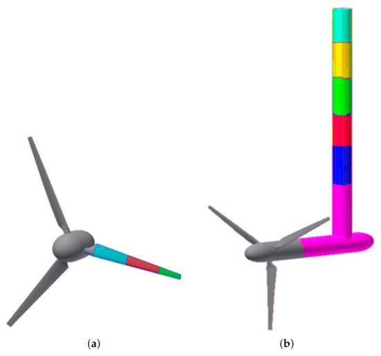
Figure 1.
HAHT geometry (a) rotor (blades and hub) and (b) support structure.

Table 1.
Summary of HAHT simulations.
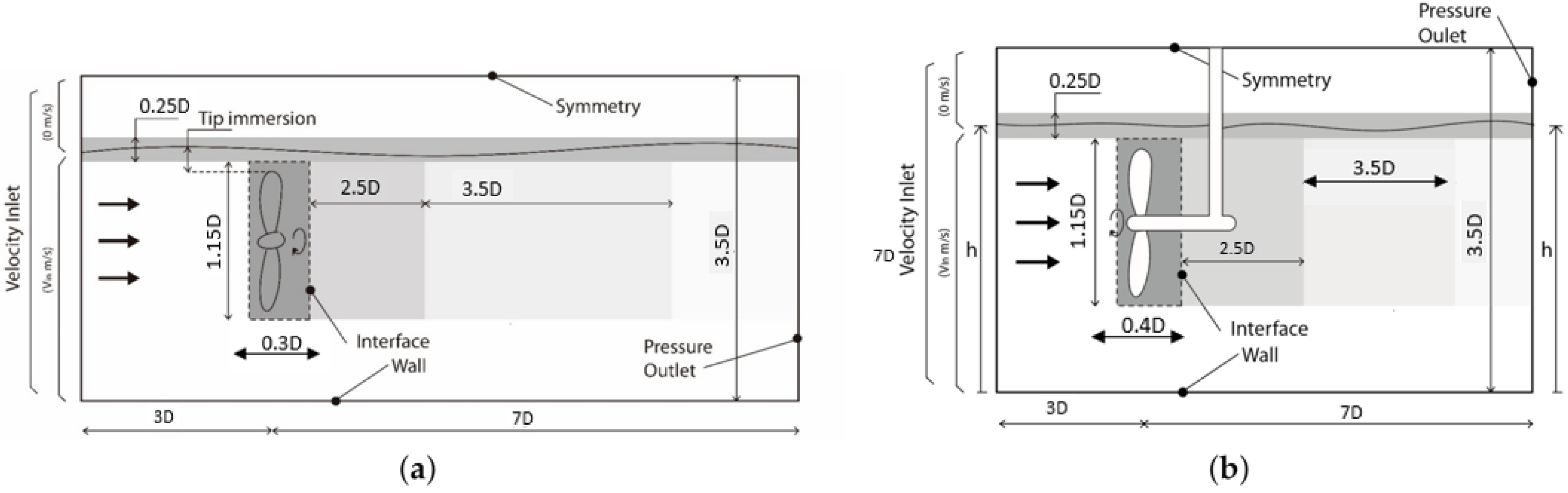
The dimensions of the computational domain are given in terms of the rotor diameter (box of ) as is shown in Figure 2. The rotor is located at a distance of 3D relative to the inlet boundary. The computational domain is divided into two subdomains, namely, an inner rotating subdomain, which encloses the rotor, and an outer stationary subdomain available to the fluid flow. The rotating and stationary subdomains share cylindrical sliding non-conformal interfaces which account for flux continuity and transient interaction effects between the two subdomains.The sliding-mesh technique implemented in the commercial CFD software ANSYS-Fluent 19.0 is used to account for the relative motion between subdomains. As a result, all cells and boundaries in the rotating subdomain revolve at the prescribed angular velocity, .
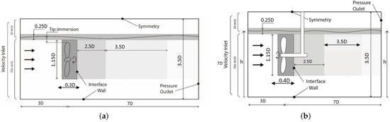
Figure 2.
Computational domain and boundary conditions considering (a) the rotor only and (b) the full turbine. Shaded areas represent mesh refinement regions.
Boundary conditions for the second and third simulated cases are shown in Figure 2a,b, respectively. At the boundary named velocity inlet, a constant velocity ( m/s) is specified on the water portion of the inlet while zero velocity is applied elsewhere. Zero gauge pressure is set at the pressure-outlet boundary; the bottom boundary is set as a stationary non-slip wall. Surfaces of the support structure are also specified as non-slip walls when the full turbine is simulated. The top and side borders are defined as zero shear slip-walls which is accomplished by a symmetry type boundary condition. Because the turbulence quantities at the inlet boundary are not known, it was decided to prescribe a moderate turbulence intensity equal to 5%. When the free surface was not considered (the first simulated case) the top, bottom, and side boundaries of the domain were set as zero shear walls moving with the same velocity as that prescribed at the inlet boundary. The rotating subdomain is a cylinder of diameter 1.15D; as it can be seen in Figure 2, the cylinder’s length is slightly increased from 0.3D to 0.4D when the support is included. The shaded areas in Figure 2 indicate mesh refinement regions. In particular, a thin region of width 0.25D is refined to better capture the free surface evolution.
2.3. Spatial and Temporal Discretization
The SIMPLE segregated solver is used together with second-order discretization schemes. The least-squares cell-based method is employed for spatial discretization of gradients. The transient formulation is set to second-order implicit. The HRIC scheme is used to discretize the convective term in Equation (2). The HRIC formulation works with an explicit upwind difference scheme to satisfy the convective boundedness criterion, so the scheme introduces some numerical diffusion due to its first-order accuracy [35].
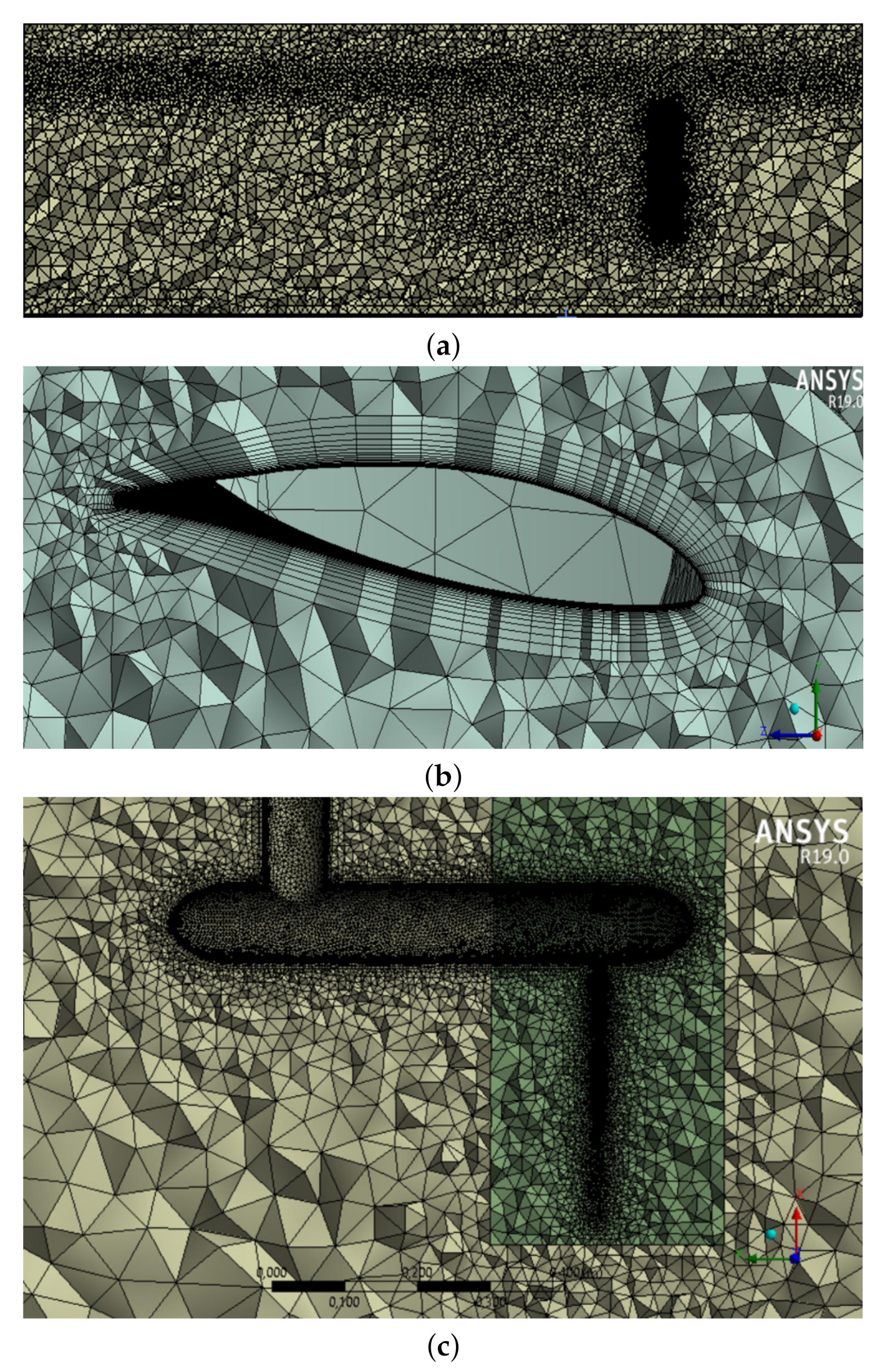
The computational domain meshed in ANSYS-Meshing 19.0 consists primarily of tetrahedral cells. A planar cut of the three-dimensional mesh is shown in Figure 3a, it corresponds to the mesh used for the second case (see Table 1). Details of the mesh around the blade are shown in Figure 3b; twenty prismatic layers are set around each blade to guarantee that the non-dimensional wall-normal coordinate lies in the viscous sublayer () and the boundary layer development is properly determined. A tetrahedral grid of a similar aspect ratio grows just outside the prismatic layer; about 85% of the computational cells are found in the rotating subdomain. A finer grid resolution is used downstream of the rotor to better capture the wake evolution. Figure 3c shows a close-up of the computational mesh around the rotor hub and support structure (case 3, Table 1). Prismatic layers are also used to capture the boundary layer effects on all structural components of the turbine.
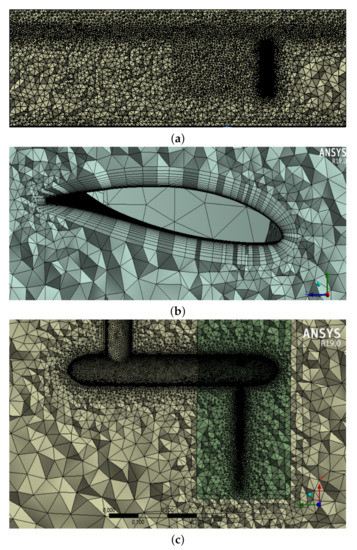
Figure 3.
Two-dimensional cut of the mesh used in (a) case 2; (b) mesh distribution around the blades; (c) details of the mesh around the support structure (case 3).
A second-order implicit scheme is used for temporal discretization. The time step is chosen so that it corresponds to a blade rotation of approximately 1°; this choice is a compromise between computational cost and accuracy. The choice of time-step size is based on a sensitivity analysis performed for case one (single-phase flow). In all cases, the calculations start with the steady MRF model to obtain a preliminary flow field, which is used as an initial condition. When the transient computation is started, first-order schemes are employed during a few time-steps before switching to second-order schemes. A maximum of 50 iterations per time step is necessary to lower the residuals below .
3. Results and Discussion
3.1. Single-Phase Flow Simulations
Single-phase flow simulations were performed to assess the sensitivity to grid resolution, time-step size, and turbulence models. Simulation results presented in this section correspond to case 1 in Table 1.
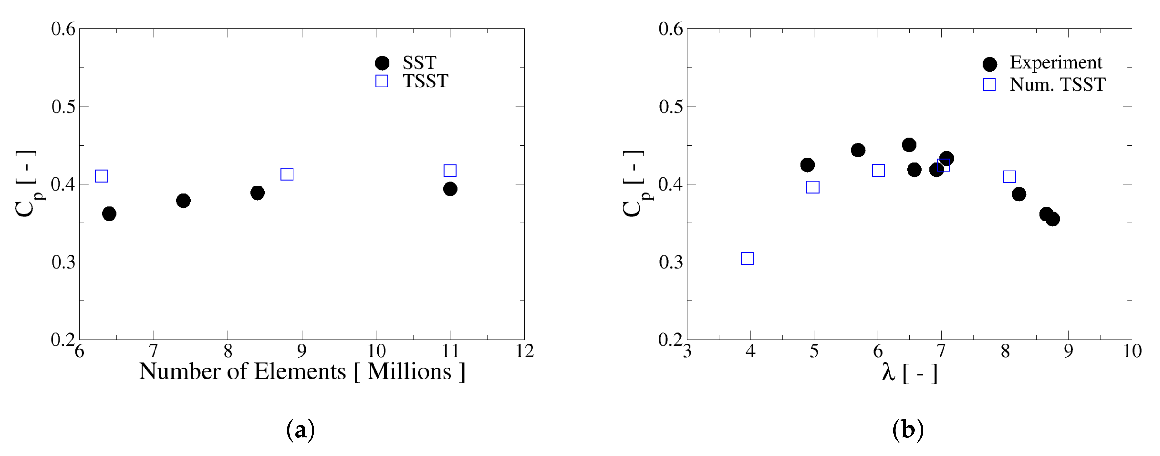
The average power coefficient obtained with the standard SST k- and the four-equation TSST models at is presented in Figure 4a. The SST k- turbulence model predicts a lower than the four-equation TSST model even when the grid is refined. When the domain is discretized with 8.5 million cells or more, the calculated with the TSST turbulence model remains approximately 5% higher than the result obtained with the SST k- model. The difference can be attributed to the ability of the TSST model to capture boundary layer transition effects which are directly related to the hydrodynamic forces acting on the rotor blades [32]. Predictions of obtained with the four-equation TSST turbulence model are compared with experimental data at various TSRs in Figure 4b. Simulation results are based on a grid resolution of 8.8 million cells and a time step of s. As it can be noticed, the numerical results slightly underestimate the experimental points and also, the simulated curve shows a small displacement toward the right regarding the measurements. However, in the range of tip speed ratios between 5 and 8, the maximum difference between the numerical and experimental points is about 6%, which at this moment constitutes a good enough agreement.

Figure 4.
Average power coefficient obtained from single-phase flow simulations. (a) Sensitivity to turbulence model at ; (b) calculated with the TSST model for various TSRs.
The effect of time-step size on the predicted power coefficient is investigated at . The instantaneous values of in time can be seen in Figure 5 whereas Table 2 shows the relationship between time-step, blade rotation, and the average . It is found that reducing the time-step size in half results in a increment of just 0.5%. Therefore, a time step of s has been chosen as a compromise between accuracy of results and simulation time; this time step corresponds to a rotation angle of 0.83° which is below the value of 1° recommended previously as a rule of thumb [26,36].
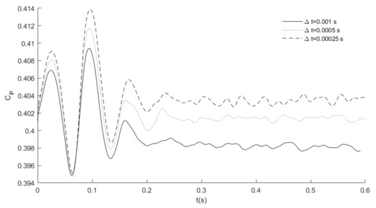
Figure 5.
Effect of time-step size on the computed at .
Table 2.
Effect of time-step size on at .
3.2. Effect of Free Surface and Support Structure on Performance
This section describes the results obtained when free surface effects and the support structure are included in the computational model. Although the support consists of a simple geometry, it increases the number of cells in the stationary subdomain by 11%. Simulation results presented in this section were computed with the four-equation TSST turbulence model.
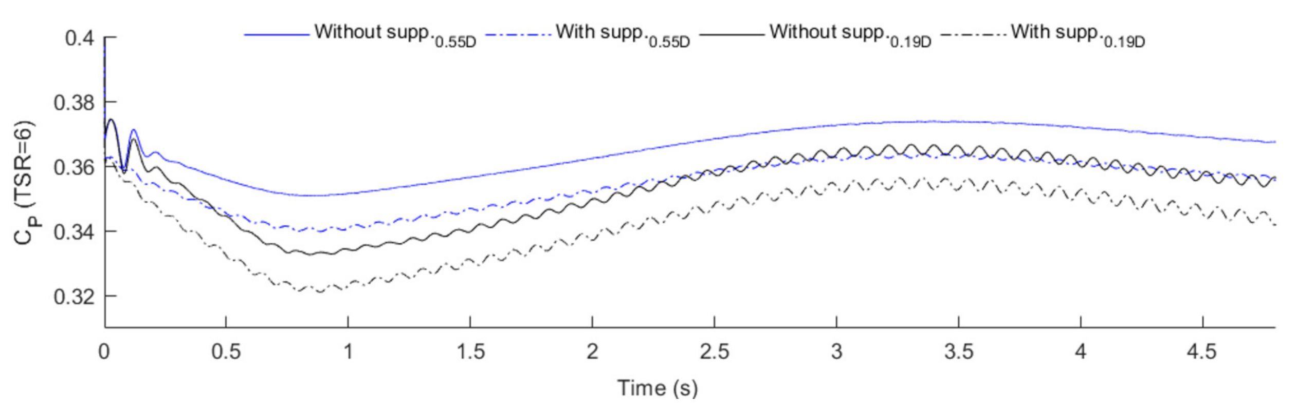
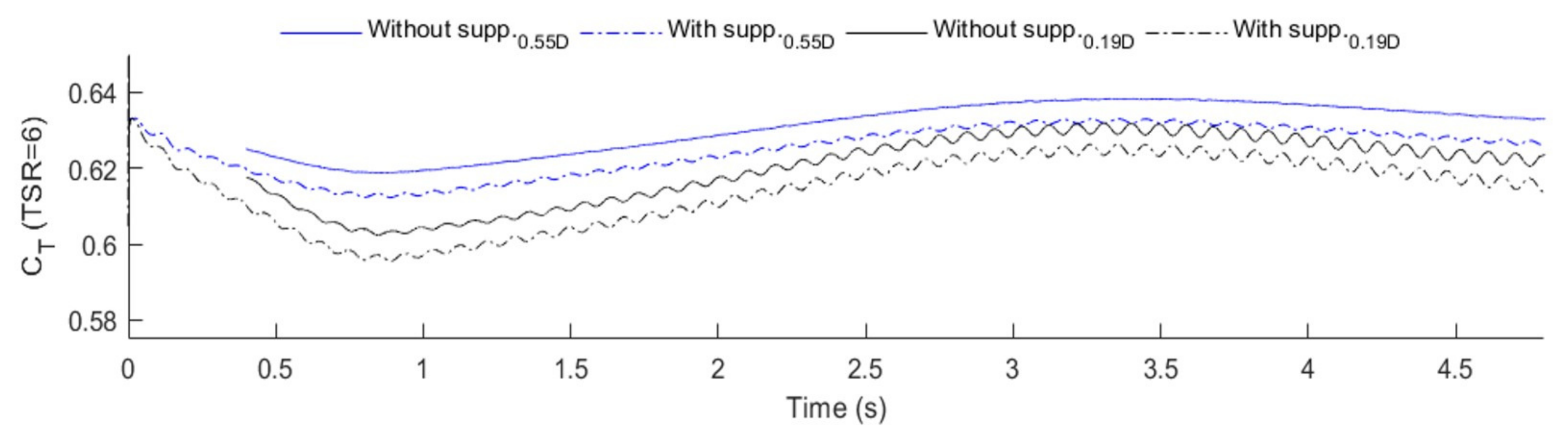
It is a fact that the presence of the free surface and its dynamics affects the performance of the turbine as well as wake development and its recovery [36]. For instance, in Kolekar et al. [19] it is concluded that the free surface compresses the wake and that it produces a blocking effect which increases for larger rotational velocities and lower tip immersions. Figure 6 and Figure 7 show the time histories of and , respectively, experienced by the blades for both, shallow and deep tip immersion cases at a TSR of 6. They are compared with the results without a support structure. In first place, it is seen that power and thrust coefficients are smaller in the shallow immersion than in the deeper configuration, a result that agrees with the observations of [18,37]. Such reduction of the coefficients is related with a stronger deformation of the free surface in the case of shallow immersion as it can be seen in Figure 8 and Figure 9 below. The interaction between this deformation and the flow behind the HAHT causes a slower wake recovery than in the case of deep immersion, which is responsible for the reduction of the turbine performance. Additionally, the presence of the support decreases further both coefficients in a similar percentage for both turbine immersions (around 3% for and 1.6% for ). Such decrease is attributed to a small flow velocity reduction caused by the presence of the supporting rod; this effect is similar to the effect of the tower on in case of horizontal wind turbines [38]. In the configuration of shallow tip immersion, the time evolution of the two coefficients display clear ripples, either considering or not the supporting structure; such ripples are due to the periodic blades passage close to the free surface and their frequency equals to that of the blades rotational frequency. On the other hand, for the deeper immersion conditions the ripples are still present but with very much attenuated amplitude, reflecting that the turbine in such configuration is close to free stream conditions. Moreover, a long period undulation in the values of the and coefficients can be appreciated in Figure 6 and Figure 7, which is present for both immersion conditions. This behavior was not seen in Yan et al. [18], where the coefficients monotonically reached a statistically steady state. The reason behind this long period coefficient undulation is at the moment not clear and deserves future investigation.
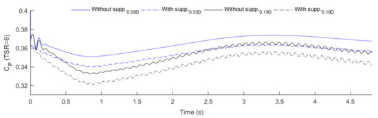
Figure 6.
Time history of power coefficient for deep and shallow tip immersions, with and without support structure. Results are for .

Figure 7.
Time history of thrust coefficient for deep and shallow tip immersions, with and without support structure. Results are for .
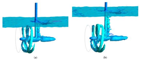
Figure 8.
Snapshots of air-water interface and vorticity isosurface of 20 Hz at (a) 0.19D and (b) 0.55D tip immersions.
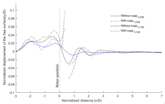
Figure 9.
Vertical displacement of the free surface at the channel mid plane. Results for and two immersions.
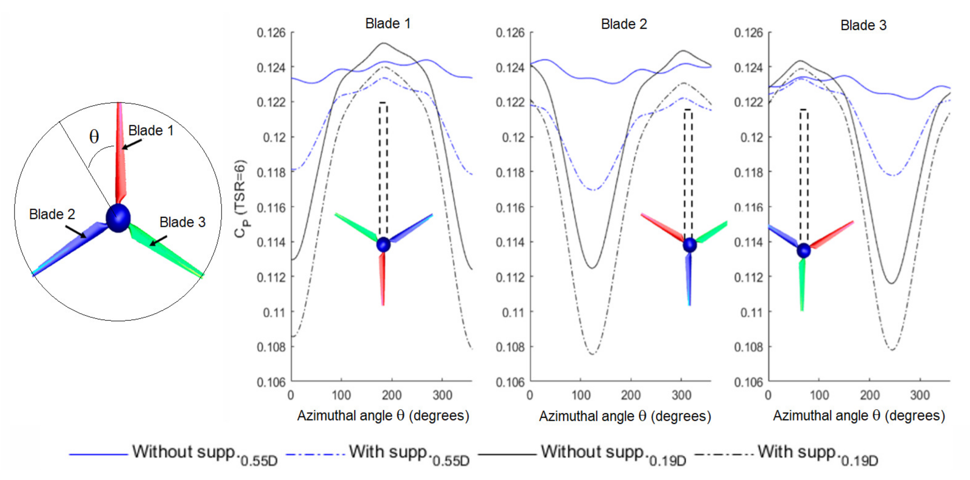
The individual contribution of each blade to the power coefficient over one revolution taking into account the effect of the support structure is shown in Figure 10. In that figure, the azimuthal angle is set at 0° when blade 1 (identified by red color) is located upwards directly pointing towards the free surface. Results correspond to a TSR of 6. The reduction in the value of for the full assembly is noted in comparison to the results when the support structure is not included in the computational model. Each blade provides the lowest when it is placed vertically upwards, aligned with the vertical bar of the support structure, and the highest when it is located vertically downwards. The difference between these two extreme values is very much reduced for the deep immersion case, regarding the shallow configuration, although it is noticeable even when the support structure is not included in the computation. Moreover, it can be observed for the case of 0.19D immersion without support that the minimum value of attained is at the position where the blade tip is closest to the free surface, a fact that illustrates that the proximity of the blades to the air-water interface greatly decrease the turbine performance, which in this case is of the same order than the presence of the supporting structure. Interestingly, the maximum value of the instantaneous power coefficient, reached when the azimuthal angle is 180°, happens for the shallow immersion configuration, regardless of the supporting rod presence.
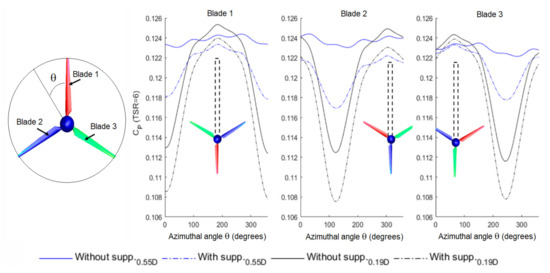
Figure 10.
Blade contribution to the power coefficient along one revolution with and without the support structure. Results are for .
The fact that the variation of along one revolution increases as the blade tip is closer to the free surface can be understood as follows. In the absence of a support structure, the flow accelerates by surrounding the blades more or less symmetrically; on the other hand, the flow through the rotor moves more slowly towards the free surface when the structure is included. This behavior is more pronounced at the shallow tip immersion. As can be seen in Figure 10, reaches its maximum when blade 1 sweeps the high flow velocity region at 180°, i.e. the blade tip is farthest from the free surface. Peak values of for blades 2 and 3 are shifted 120° and 240°, respectively. The support structure lowers the contribution of blade 1 to when the blade is pointing upwards (at 0°) and the difference between the curves with and without support structure is the highest. It resembles the tower shadow effect experienced by horizontal axis wind turbine blades, which is known to be the main cause of power fluctuation [38].
3.3. Wake and Free Surface Interactions
Figure 8 shows the vorticity isosurface (20 Hz) and free surface for both deep and shallow tip immersion simulations in the case which includes the supporting structure. Significant deformation of the air-water interface can be observed at both tip immersions, especially in the vicinity of the support rod. Figure 8 shows the wake past the support structure, revealed by the vorticity isosurface, which could not be detected in the previous study of Yan et al. [18] but is present in the recent work of [37]. As a comment, blade root vortices are observed in the results of [18], which can be attributed to the presence of a gap between the rotor and the support in the employed computational model. That space is not considered in this work, so the horizontal part of the support hinders the development of root vortices in the present case.
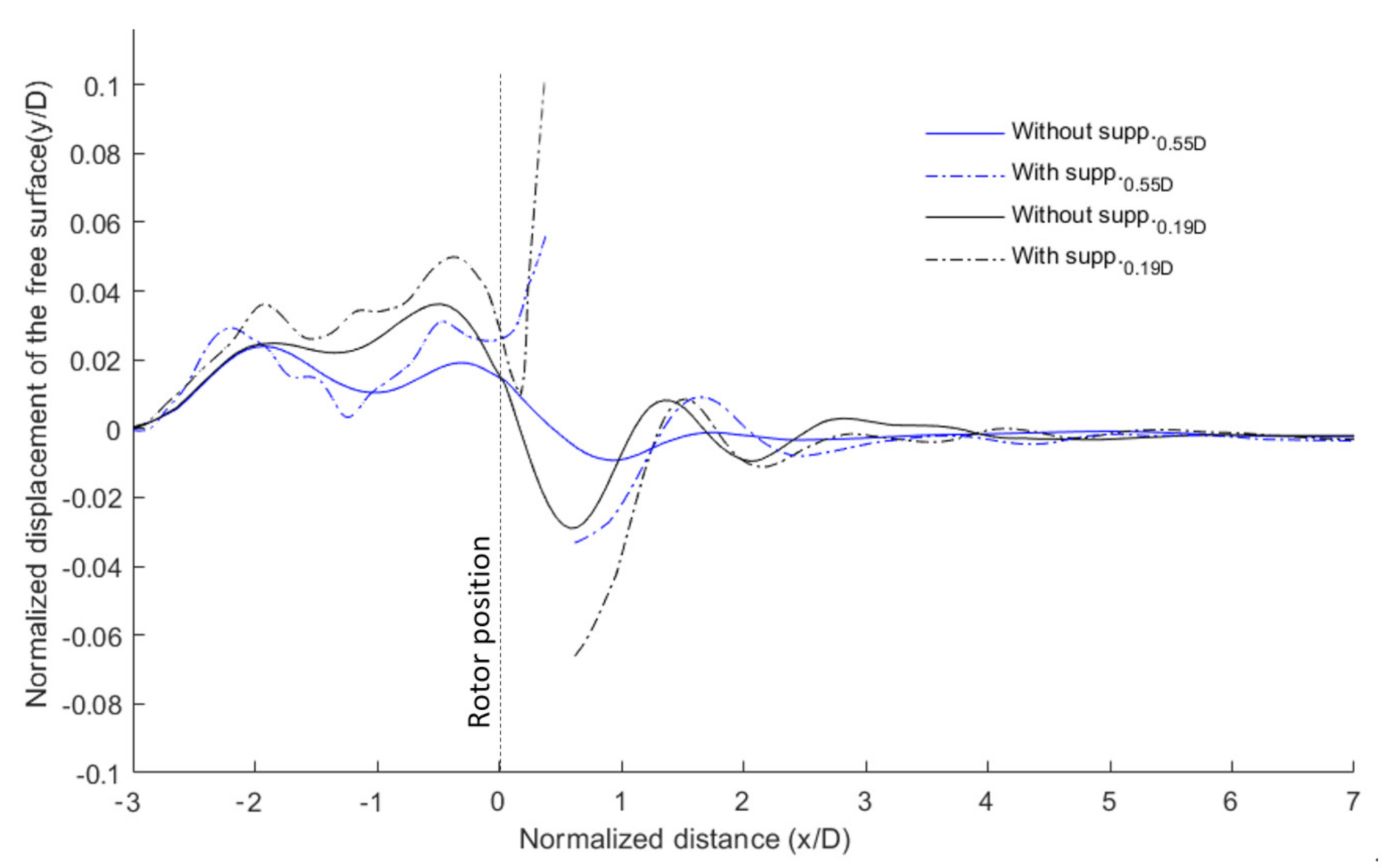
The vertical displacement of the free surface at the domain mid-plane is presented in Figure 9. The displacement is normalized by the rotor diameter for both the shallow and deep tip immersions. Time-averaged results were obtained in the last three revolutions for . The configuration without support, solid lines in Figure 9, induces an elevation of the water level just upstream the rotor and a gentle drop of it downstream. This effect is of course due to the obstruction generated by the turbine in the flow and it is more pronounced in the shallow immersion. On the other hand, the inclusion of the support structure causes a discontinuity immediately downstream of the rotor position; the surface rapidly elevates in front of the pole (vertical rod) while a sort of dimple forms just downstream. Two peaks are observed upstream regardless of the presence of the structure. Moreover, the free surface deformation upstream is increased for both immersions when the structure is included in the model. For the deep tip immersion, the free surface exhibits little disturbance downstream from the rotor in the absence of the structure which suggests that the free surface effect on the rotor performance is marginal when the rotor is well below it, in agreement with the conclusions of [18,37]. The highest depression downstream on the free surface occurs for the 0.19D immersion when the structure is present, followed by a peak that is approximately equal for both deep and shallow immersions with the support structure. In order to provide a quantitative estimation, the normalized maximum free-surface displacement () and its location downstream relative to the rotor position () are summarized in Table 3. The results are compared with interpolated data taken from the study of Adamski [22]. Froude number () is based on the rotor diameter and represents the rotor depth-to-diameter ratio. As it can be seen, the computed maximum displacement agrees reasonably well with the results reported by [22] for both tip immersions.
Table 3.
Normalized maximum displacement of the free surface () and its location downstream the rotor ().
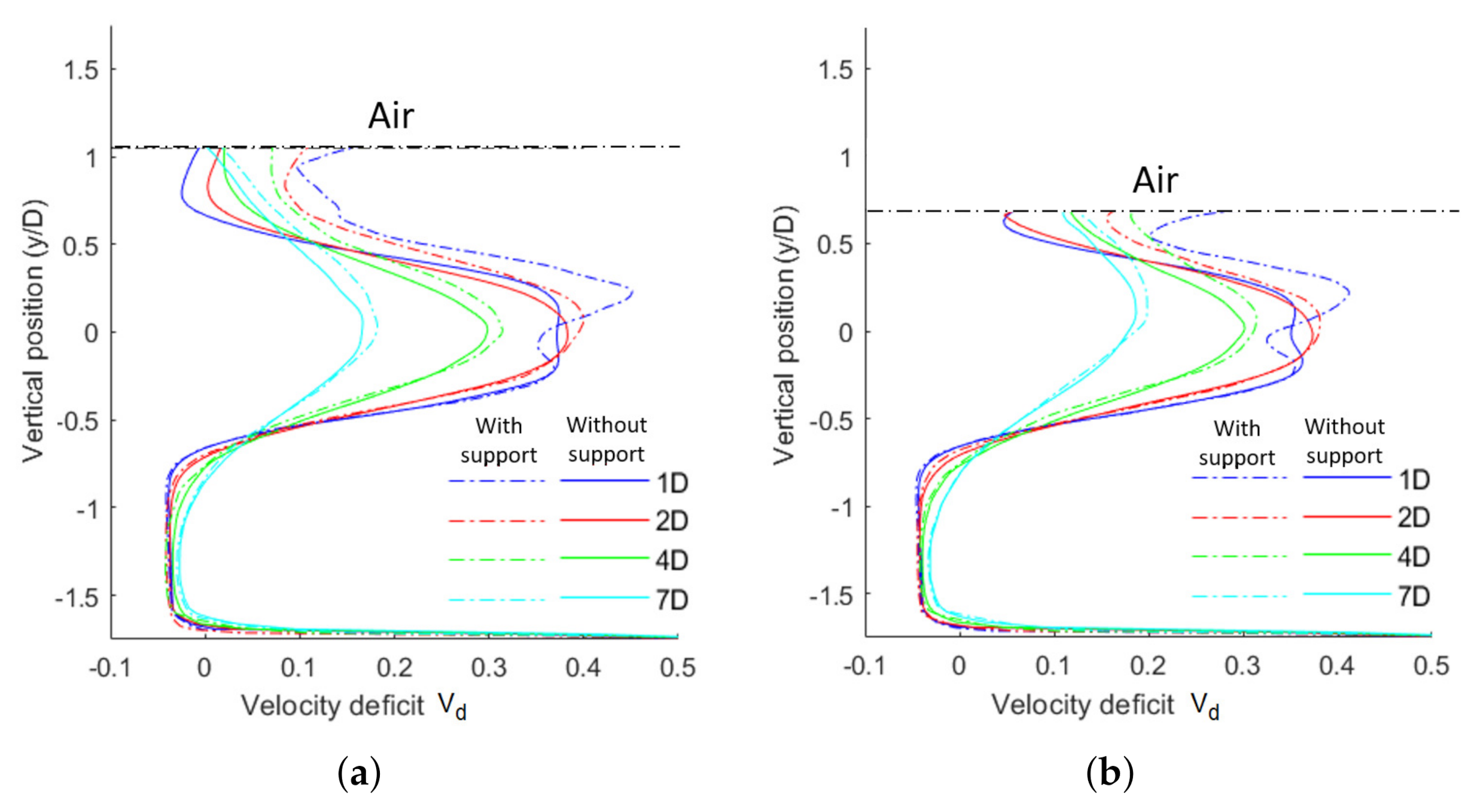
On the other hand, the study of wake development is of importance to determine the optimal spacing between HAHTs in a hydrokinetic farm [11,39,40,41]. Time-averaged velocity deficit profiles downstream of the simulated HAHT are shown in Figure 11a and Figure 11b for the deep tip and shallow tip immersions, respectively. The profiles are taken from the vertical center plane so corresponds to the rotor centerline. The dot-dashed horizontal line represents the level of the undisturbed free surface. Profiles are shown at four positions downstream of the HAHT; a comparison is drawn between the combined effect of the rotor and support structure on the wake and in the absence of a support structure (case 2 in Table 1). Significant differences between the profiles can be appreciated, especially in the near wake region (at a distance less than from the rotor). At , the maximum velocity deficit is found off the centerline both for the deep-tip and shallow tip immersions when the support structure is included. The corresponding curves in this case show two unequal peaks instead of the two symmetric maximums in the case without supporting structure. Simulation results suggest that the support shifts the maximum velocity deficit towards the free surface line, a fact clearly observed in Figure 11b for the shallow immersion configuration. It can be also noticed that the combined effect of rotor and support structure reduces the velocity in the wake above the rotor centerline for the analyzed positions and tip immersions. Due to the free surface proximity, the wake recovers somewhat slower when the tip immersion is 0.19D. In this case, the wake expansion is quickly constrained by the free surface, which in turn reduces the power and thrust coefficients at shallow tip immersions.
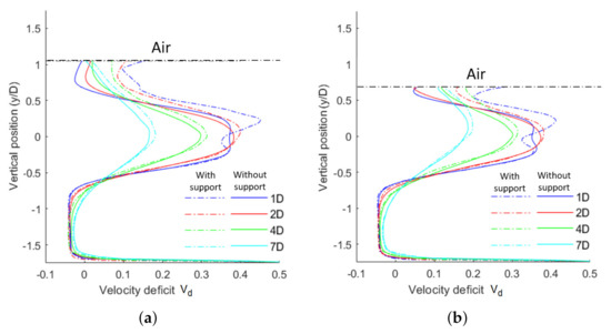
Figure 11.
Comparison of time-averaged velocity deficit profiles at four downstream positions of the HAHT at . (a) Deep tip immersion (); (b) Shallow tip immersion ().
4. Conclusions
A computational study of the influence of the free surface and supporting structure on the flow around a HAHT was conducted using the VOF method combined with the sliding mesh technique and RANS turbulence models. The commercial CFD software ANSYS-Fluent 19.0 was used to implement the computational model. First, the HAHT performance was analyzed in the absence of the free surface and without the support structure. Computations showed that the four-equation TSST turbulence model led to predictions of which are in better agreement with the experimental results of Bahaj et al. [17] for TSRs between 4 and 8 than those obtained with the standard SST model. A thorough sensitivity analysis showed that a mesh with about eight million cells and a time-step of about s are required to estimate the power and thrust coefficients within a reasonable computing time. Then, the performance was analyzed by taking into account the free surface in the computational domain. The rotor was placed at two tip immersions showing that a shallow immersion results in lower power extraction in agreement with experimental results. In addition, predictions of power and thrust coefficients were found to be affected by the support structure. Also, the dynamics of the wake behind the turbine was shown to be affected by both the free surface and the presence of the support structure. In the shallow immersion case, the development of the wake is constrained by the free surface and supporting structure leading to a slower wake recovering and to a decrease of the turbine power coefficient.
Future work will explore the overset mesh technique to replace the sliding non-conformal interface currently used for the interpolation between stationary and rotating subdomains. The simulation of very shallow turbine immersions is also planned, where the blades emerge above the free surface, inclusive of fluid-structure interaction and the possible appearance of cavitation effects.
Author Contributions
Conceptualization, A.B.-M. and S.L.; methodology, A.B.-M. and S.L.; validation, L.R.-J.; formal analysis, L.R.-J., A.B.-M. and S.L.; investigation, L.R.-J.; resources, S.L.; data curation, L.R.-J.; writing—original draft preparation, A.B.-M.; writing—review and editing, S.L. and L.R.-J.; visualization, L.R.-J.; supervision, A.B.-M. and S.L. All authors have read and agreed to the published version of the manuscript.
Funding
This research received no external funding.
Institutional Review Board Statement
Not applicable.
Informed Consent Statement
Not applicable.
Data Availability Statement
The data presented in this study are available on request from the corresponding author.
Acknowledgments
The authors thank the financial support provided by the Research Vice-rectory of Universidad Autónoma de Occidente. We acknowledge the use of the ANSYS license and computer time provided by the Laboratorio de Bioprocesos y Flujos Reactivos (BIOFRUN) at the Facultad de Minas of the Universidad Nacional de Colombia.
Conflicts of Interest
The authors declare no conflict of interest.
Abbreviations
The following abbreviations are used in this manuscript:
| HAHT | Horizontal Axis Hydrokinetic Turbine |
| HRIC | High Resolution Interface Capturing |
| SIMPLE | Semi-Implicit Method for Pressure-Linked Equations |
| MRF | Moving Reference Frame |
| TSR | Tip Speed Ratio |
| TSST | Transition Shear Stress Transport |
| URANS | Unsteady Reynolds Average Navier-Stokes |
References
- International Energy Agency. Available online: https://www.iea.org (accessed on 30 August 2021).
- Rogers, J.D. Celebrating Hoover Dam: The Majesty of Hoover Dam. Civ. Eng. Mag. 2010, 80, 52–65. [Google Scholar] [CrossRef]
- Suárez, B.; Vera Rodríguez, J.D.; Botero, F.; Suárez Agudelo, B.H.; Giraldo Jiménez, W. Hidroituango Intake Gate Closure—Emergency Conditions. Revista Facultad de Ingeniería Universidad de Antioquia 2021. Available online: https://revistas.udea.edu.co/index.php/ingenieria/article/view/344363 (accessed on 10 September 2021).
- Organization for Economic Co-operation and Development. Available online: https://stats.oecd.org (accessed on 28 August 2021).
- Anyi, M.; Kirke, B. Evaluation of small axial flow hydrokinetic turbines for remote communities. Energy Sustain. Dev. 2010, 14, 110–116. [Google Scholar] [CrossRef]
- Batten, W.; Bahaj, A.; Molland, A.; Chaplin, J. The prediction of the hydrodynamic performance of marine current turbines. Renew. Energy 2008, 33, 1085–1096. [Google Scholar] [CrossRef]
- Lee, J.H.; Park, S.; Kim, D.H.; Rhee, S.H.; Kim, M.C. Computational methods for performance analysis of horizontal axis tidal stream turbines. Appl. Energy 2012, 98, 512–523. [Google Scholar] [CrossRef]
- Batten, W.; Bahaj, A.; Molland, A.; Chaplin, J. Experimentally validated numerical method for the hydrodynamic design of horizontal axis tidal turbines. Ocean. Eng. 2007, 34, 1013–1020. [Google Scholar] [CrossRef]
- Danao, L.A.; Abuan, B.; Howell, R. Design Analysis of a Horizontal Axis Tidal Turbine. In Proceedings of the 3rd Asian Wave and Tidal Conference-AWTEC, Singapore, 24–28 October 2016. [Google Scholar]
- Bowman, J.; Bhushan, S.; Thompson, D.S.; O’Doherty, D.; O’Doherty, T.; Mason-Jones, A. A physics-based actuator disk model for hydrokinetic turbines. In Proceedings of the Fluid Dynamics Conference, Atlanta, GA, USA, 25–29 June 2018. [Google Scholar]
- Silva dos Santos, I.F.; Camacho, R.G.R.; Filho, G.L.T. Study of the wake characteristics and turbines configuration of a hydrokinetic farm in an Amazonian river using experimental data and CFD tools. J. Clean. Prod. 2021, 229, 126881. [Google Scholar]
- Mikkelsen, R. Actuator Disc Methods Applied to Wind Turbines. Ph.D. Thesis, Technical University of Denmark, Lyngby, Denmark, 2003. [Google Scholar]
- Sørensen, J.N.; Shen, W.Z. Numerical Modeling of Wind Turbine Wakes. ASME J. Fluids Eng. 2002, 124, 393–399. [Google Scholar] [CrossRef]
- Henao Garcia, S.; Benavides-Morán, A.; Lopez Mejia, O.D. Wake and Performance Predictions of Two- and Three-Bladed Wind Turbines Based on the Actuator Line Model. ASME J. Fluids Eng. 2021, 143, 051206. [Google Scholar] [CrossRef]
- Baba-Ahmadi, M.H.; Dong, P. Validation of the actuator line method for simulating flow through a horizontal axis tidal stream turbine by comparison with measurements. Renew. Energy 2017, 113, 420–427. [Google Scholar] [CrossRef] [Green Version]
- Hocine, A.E.B.L.; Jay, R.W.; Poncet, S. Multiphase modeling of the free surface flow through a Darrieus horizontal axis shallow-water turbine. Renew. Energy 2019, 143, 1890–1901. [Google Scholar] [CrossRef]
- Bahaj, A.; Molland, A.F.; Chaplin, J.R.; Batten, W.M.J. Power and thrust measurements of marine current turbines under various hydrodynamic flow condition in a cavitation tunnel and a towing tank. Renew. Energy 2007, 32, 407–423. [Google Scholar] [CrossRef]
- Yan, J.; Deng, X.; Korobenko, A.; Bazilevs, Y. Free-surface flow modeling and simulation of horizontal-axis tidal-stream turbines. Comput. Fluids 2017, 158, 157–166. [Google Scholar] [CrossRef]
- Kolekar, N.; Vinod, A.; Banerjee, A. On Blockage Effects for a Tidal Turbine in Free Surface Proximity. Energies 2019, 12, 3325. [Google Scholar] [CrossRef] [Green Version]
- Nishi, Y.; Sato, G.; Shiohara, D.; Inagaki, T.; Kikuchi, N. Performance characteristics of axial flow hydraulic turbine with a collection device in free surface flow field. Renew. Energy 2017, 112, 53–62. [Google Scholar] [CrossRef]
- Bai, X.; Avital, E.J.; Munjiza, A.; Williams, J.J.R. Numerical simulation of a marine current turbine in free surface flow. Renew. Energy 2014, 63, 715–723. [Google Scholar] [CrossRef]
- Adamski, S.J. Numerical Modeling of the Effects of a Free Surface on the Operating Characteristics of Marine Hydrokinetic Turbines. Master’s Thesis, University of Washington, Seatle, GA, WA, 2013. [Google Scholar]
- Rodríguez, L.; Benavides-Moran, A.; Laín, S. Three-Bladed Horizontal Axis Water Turbine Simulations with Free Surface Effects. Int. J. Appl. Mech. Eng. 2021, 26, 187–197. [Google Scholar] [CrossRef]
- Hirt, C.W.; Nichols, B.D. Volume of fluid (VOF) method for the dynamics of free boundaries. J. Comput. Phys. 1981, 39, 201–225. [Google Scholar] [CrossRef]
- Menter, F.R. Zonal two equation k-turbulence models for aerodynamic flows. In Proceedings of the 23rd Fluid Dynamics, Plasmadynamics and Lasers Conference, Orlando, FL, USA, 6–9 July 1993. [Google Scholar]
- Contreras, L.T.; López, O.D.; Laín, S. Computational fluid dynamics modelling and simulation of an inclined horizontal axis hydrokinetic turbine. Energies 2018, 11, 3151. [Google Scholar] [CrossRef] [Green Version]
- Langtry, R.B.; Menter, F.R. Transition Modeling for General CFD Applications in Aeronautics. In Proceedings of the 43rd AIAA Aerospace Sciences Meeting and Exhibit, Reno, NV, USA, 10–13 January 2005. [Google Scholar]
- Langtry, R.B.; Menter, F.R.; Likki, S.R.; Suzen, Y.B.; Huang, P.G.; Völker, S. A Correlation-Based Transition Model Using Local Variables—Part II: Test Cases and Industrial Applications. ASME J. Turbomach. 2006, 128, 423–434. [Google Scholar] [CrossRef]
- Rezaeiha, A.; Montazeri, H.; Blocken, B. On the accuracy of turbulence models for CFD simulations of vertical axis wind turbines. Energy 2019, 180, 838–857. [Google Scholar] [CrossRef]
- Arab, A.; Javadi, M.; Anbarsooz, M.; Moghiman, M. A numerical study on the aerodynamic performance and the self-starting characteristics of a Darrieus wind turbine considering its moment of inertia. Renew. Energy 2017, 107, 298–311. [Google Scholar] [CrossRef]
- Almohammadi, K.M.; Ingham, D.B.; Ma, L.; Pourkashanian, M. Modeling dynamic stall of a straight blade vertical axis wind turbine. J. Fluids Struct. 2015, 57, 144–158. [Google Scholar] [CrossRef]
- Laín, S.; Taborda, M.A.; López, O.D. Numerical study of the effect of winglets on the performance of a straight blade Darrieus water turbine. Energies 2018, 11, 297. [Google Scholar] [CrossRef] [Green Version]
- López, O.; Meneses, D.; Quintero, B.; Laín, S. Computational study of transient flow around Darrieus type Cross Flow Water Turbines. J. Renew. Sustain. Energy 2016, 8, 014501. [Google Scholar] [CrossRef]
- Myers, L.; Bahaj, A.S. Near wake properties of horizontal axis marine current turbines. In Proceedings of the 8th European Wave and Tidal Energy Conference-EWTEC, Upsala, Sweden, 7–10 September 2009. [Google Scholar]
- Waclawczyk, T.; Koronowicz, T. Comparison of CICSAM and HRIC high-resolution schemes for interface capturing. J. Theor. Appl. Mech. 2008, 46, 325–345. [Google Scholar]
- El Fajri, O.; Bowman, J.; Bhushan, S.; Thompson, D.; O’Doherty, T. Numerical study of the effect of tip-speed ratio on hydrokinetic turbine wake recovery. Renew. Energy 2022, 182, 725–750. [Google Scholar] [CrossRef]
- Tian, W.; Ni, X.; Mao, Z.; Zhang, T. Influence of surface waves on the hydrodynamic performance of a horizontal axis ocean current turbine. Renew. Energy 2020, 158, 37–48. [Google Scholar] [CrossRef]
- Wen, B.; Wei, S.; Wei, K.; Yang, W.; Peng, Z.; Chu, F. Power fluctuation and power loss of wind turbines due to wind shear and tower shadow. Front. Mech. Eng. 2017, 12, 321–332. [Google Scholar] [CrossRef] [Green Version]
- Müller, S.; Muhawenimana, V.; Wilson, C.A.M.E.; Ouro, P. Experimental investigation of the wake characteristics behind twin vertical axis turbines. Energy Convers. Manag. 2021, 247, 114768. [Google Scholar] [CrossRef]
- Myers, L.; Bahaj, A.S. Experimental analysis of the flow field around horizontal axis tidal turbines by use of scale mesh disk rotor simulators. Ocean. Eng. 2010, 37, 218–227. [Google Scholar] [CrossRef]
- Silva, P.A.S.F.; De Oliveira, T.F.; Junior, A.C.P.B.; Vaz, J.R.P. Numerical Study of Wake Characteristics in a Horizontal-Axis Hydrokinetic Turbine. Ann. Braz. Acad. Sci. 2016, 88, 2441–2456. [Google Scholar] [CrossRef] [PubMed] [Green Version]


Publisher’s Note: MDPI stays neutral with regard to jurisdictional claims in published maps and institutional affiliations. |
© 2021 by the authors. Licensee MDPI, Basel, Switzerland. This article is an open access article distributed under the terms and conditions of the Creative Commons Attribution (CC BY) license (https://creativecommons.org/licenses/by/4.0/).