
Optimal Design Method for Static Precision of Heavy-Duty Vertical Machining Center Based on Gravity Deformation Error Modelling

1
School of Mechanical Engineering, University of Shanghai for Science and Technology, Shanghai 200093, China
2
Department of Mechanical and Aerospace Engineering, Brunel University London, Uxbridge UB8 3PH, UK
3
R&D Centre, Wuhan Second Ship Design & Research Institute, Wuhan 430205, China
*
Author to whom correspondence should be addressed.
Processes 2022, 10(10), 1930; https://doi.org/10.3390/pr10101930
Submission received: 6 September 2022
/
Revised: 19 September 2022
/
Accepted: 21 September 2022
/
Published: 24 September 2022
(This article belongs to the Section Manufacturing Processes and Systems)
Abstract
:Due to the large size and large span of heavy-duty machine tools, the structural deformation errors caused by gravity account for a large proportion of the static errors, and the influence of gravity deformation must thus be considered in the machine tool precision design. This paper proposes a precision design method for heavy-duty vertical machining centers based on gravity deformation error modelling. By abstracting the machine tool into a multibody system topology, the static error model of the machine tool is established based on the multibody system theory and a homogeneous coordinate transformation. Assuming that the static error of each motion axis is composed of two parts, i.e., the manufacturing-induced geometric error and the gravity deformation error, the machine tool stiffness model of the relationship between gravity and deformation error is developed using the spatial beam elements. In the modelling process, the stiffness coefficients and volume coefficients of the components are introduced to fully consider the influences of structural parameters on machine tool precision. Taking the machine tool static precision, the component stiffness coefficients and the volume coefficients as the design variables, based on the use of the worst condition method, error sensitivity analysis and global optimization algorithm, the optimal allocation of the static error budget of the machine tool and the structural design requirements of each component are determined, providing a valuable guide for the detailed structure design and manufacture processing of the machine tool components.
1. Introduction
Heavy-duty computer numerical control (CNC) machine tools are widely used in national defense, aerospace, energy and other key fields for machining large workpieces. The level of machining precision is one of the most important indicators of the performance of heavy-duty CNC machine tools. The factors that affect the machining precision of CNC machine tools include geometric errors, thermal errors, cutting force errors, servo control errors, etc. Amongst them, geometric errors and thermal errors account for 60% of the total machining errors [1]. However, heavy-duty CNC machine tools have structural characteristics such as a large size and large span. The influence of gravity-induced deformation error on machining precision is more prominent and significant than for common CNC machine tools, occupying a larger proportion of the static errors [2]. How to address the effects of the gravity and quantitatively analyze the influences of structural deformation errors on the precision is a problem that needs to be solved in the precision design of heavy-duty CNC machine tools.
Error modelling is a key step in the static precision design of machine tools. By analyzing the causes and mechanisms of each error, a model mapping each error to the volumetric error of the tool center point (TCP) is established, which allows the prediction of the machining error of the machine tool to be realized and provides a theoretical basis for rational error budgeting. The multibody system (MBS) theory and the homogeneous transformation matrix (HTM) method are widely applied to model the volumetric errors of the multiaxis machine tool for error prediction and compensation [3,4,5,6]. Fu et al. proposed an optimal compensation method based on the rigid body geometric error model to improve the precision of a five-axis machine tool and identified the critical motion axes that affected the machine tool precision through a sensitivity analysis [7,8]. Wu et al. established a geometric error model for nonorthogonal five-axis machine tools and constructed the mapping relationship between the tool path and NC commands under the influence of geometric errors during the machining process [9]. Breitzke et al. proposed a method to quickly identify geometric errors of three-axis machine tools using on-machine measurement samples [10]. Gu et al. proposed a method for improving machine tool precision based on a global offset, utilizing sample inspection data to determine specific compensation parameters used in the machine tool controller to minimize machine tool errors [11]. Iñigo et al. proposed a digital twin-based machine tool accuracy calibration simulation method, its expected error range and parameters such as workpiece geometry on the uncertainty of error mapping [12]. The above research works show that deriving the volumetric error of the TCP by HTM and MBS is still the main idea of machine tool error modelling.
Although the current research studies are mostly focused on the error compensation, in fact, the establishment of the above error models have provided a research basis for precision design research. Chen established a five-axis ultraprecision machine tool precision model by using MBS and HTM and proposed static and dynamic precision design methods [13,14]. Based on the relationship between the guideway surface tolerance and the surface geometry and the geometric errors of the motion axes, Fan et al. further discussed a method for predicting the geometric errors of the machine tool motion axes to guide the precision allocation of the machine tool [15,16]. Xu et al. performed the precision design for a six-axis CNC spiral bevel gear milling machine according to the workpiece precision requirements [17]. Li and Liu analyzed the sensitivity of each error source of the machine tool by the proposed generalized sensitivity index [18]. Li et al. used a heuristic algorithm to allocate the errors of the five-axis machine tool [19]. Zhang et al. proposed a precision design method considering manufacturing cost and reliability [20]. The response surface and artificial neural network was also used to predict the performance of machine tool, helping to design the parameters of interest through optimization [21]. In the above research, the static precision design/allocation problem of machine tool is equivalent to a nonlinear optimization problem combining the influences of various error factors, and the design output is the optimal precision requirement after the machine tool is assembled, guiding the assembly and testing of machine tools. However, for heavy-duty machine tools, the effects of the gravity make this precision requirement not optimal anymore. According to the precision requirement optimized without the consideration of the gravity-induced deformation error, it will be costly if the assurance of the machine tool precision only occurs at the assembly stage. Therefore, to eliminate the status quo of over-reliance on the assembly stage for heavy-duty machine tools is an urgent problem to solve in the precision design.
Due to the large size and large span of a heavy-duty machine tool, the error modelling process of the heavy-duty machine tool should consider the gravity deformation error under static conditions and its influence on the volumetric error of the machine tool’s TCP. Yan et al. proposed a semianalytical method based on the closed-loop stiffness model of a multiaxis system to describe the comprehensive stiffness characteristics of the machine tool system [22]. Portman et al. developed the stiffness model of multiaxis machine tools through the form-shaping function [23]. Based on the principle of six-point positioning, Ma et al. proposed a linear axis assembly error model of CNC machine tools to analyze the influences of processing errors and deformation to guide the precision design of the machine tool [24]. Shi et al. used static loading to simulate the cutting force under different milling conditions and combined this with the HTM error model to develop a three-axis machine tool error compensation method based on equivalent cutting force [25]. Shi et al. proposed a top-down stiffness design of the machine tool by using stiffness coefficients to characterize the stiffness of structural components and functional units [26]. However, the above research studies are all oriented to machine tools with definite structures, and their stiffness modelling methods are highly specific to the already designed structures and cannot thus provide a theoretical guidance for the precision design and structural design of machine tools at the design stage.
In order to solve the above-mentioned problems, this paper comprehensively considers the sources and interrelations of various error factors, determines the optimal precision requirements in the design and manufacturing stages, and develops a method for the precision design of a heavy-duty machine tool based on the gravity error modelling, with the implementation process of the design method explained using a heavy-duty vertical machining center (HDVMC) as an example. This paper is organized as follows. Section 2 analyzes the design process step by step and clarifies the methods and processes. Section 3 abstracts the machine tool as an MBS topology and establishes the static precision model of the machine tool based on the MBS theory and HTM method. Section 4 considers the influence of the gravity deformation on the precision of the heavy-duty machine tool. Assuming that the static error is composed of the manufacturing-induced geometric error and the gravity deformation error, the stiffness coefficient and the volume fraction are introduced, and the spatial beam element is used to establish a machine tool stiffness model describing the relationship between gravity deformation error and static error. Section 5 takes the machine tool static precision, the component stiffness coefficient and the volume fraction as the design variables, and combines the worst-condition method, an error sensitivity analysis and a global optimization algorithm to formulate a mathematical model of static precision design. Section 6 completes the optimal design of the key parameters of the structural design of each component, matches the manufacturing and processing tolerances of key components, clarifies the design process and method and compares it with the existing design methods for verification.
2. Precision Design Method of Heavy-Duty Machine Tool Based on Gravity Deformation Error Modelling
This paper proposes a static precision design method for HDVMCs based on gravity deformation error modelling. The main feature of the method is that the 37 static errors of the heavy-duty machine tool and the structural parameters of each machine component are allocated by a coupling calculation, and the static precision is guaranteed on the basis of satisfying the structural design requirements of each component of the heavy-duty machine tool and its deformation. The flowchart is shown in Figure 1.
In this precision design method, the geometric error model and the gravity deformation error model of the machine tool are first established, and the objective function and constraint conditions of the precision design problem are analyzed and computed in combination with the error sensitivity. After the optimization, the sensitivity analysis of the errors is performed again to determine the important errors, providing a guide for the design and manufacture of machine tool components. If necessary, after each optimal allocation, a partial adjustment of some errors can also be carried out based on the engineering experience. The sensitivity analysis is used as the reference for the error adjustment, and finally the rational error budgeting is realized through multiple allocations. If a feasible solution cannot be obtained with this displacement constraint, it means that the error caused by the gravity deformation in the design scheme is too large, and the static precision required by the precision design cannot be achieved. It is necessary to modify the value range of the structural parameters in the design variables, or to carry out process measures, such as reverse deformation processing of the bearing surface and balance weight for the components with large deformation, to correct the errors caused by gravity deformation, and continue to optimize.
3. Modelling of Machine Tool Static Error Based on Multibody System
The MBS model is directly related to the specific kinematics of the machine tool. In this paper, a HDVMC was used as an example to establish a multibody kinematics model. The machine tool had four linear motion axes and one rotary motion axis, and its three-dimensional model is shown in Figure 2. The movement strokes of X-, Y-, Z- and W-axes were 3700 mm, 2200 mm, 1000 mm and 1000 mm, respectively, the maximum machining diameter could reach 1600 mm, and the maximum weight of workpiece could reach 8 t.
3.1. Machine Tool Topology and Coordinate System
According to the machine tool structure in Figure 2, the MBS topology is abstracted from the relationship between the moving parts in the kinematic chain. As shown in Figure 3, the MBS consists of multiple bodies Bj (j = 1, 2, …, 9) and hinges hi (i = 1, 2, …, 9), each hinge has only two bodies connected, and the fixed part is the bed of the machine tool, which is represented by B1. There are two kinematic chains in the machine tool, namely the bed-workpiece chain (B1, B7~B9) and the bed-tool chain (B1~B6). The endpoints of the two kinematic chains are the tool processing point and the workpiece point being processed. The volumetric error of the system is the difference between the actual and theoretical processing points of the tool.
To clearly explain the kinematic relationship of the MBS, the inertial reference system and body-fixed coordinate systems need to be established. The origin O0 of the inertial reference system O0–X0Y0Z0 is located at the connection between the earth and the machine bed, and its coordinate axes are parallel to the nominal directions of the X-, Y-, and Z-axes of the machine tool, conforming to the right-hand rule. It is a set of Cartesian coordinate systems fixed to an immovable reference object. The coordinate origin Oj of the body-fixed coordinate system Oj–XjYjZj on the body Bj is set on the inscribed hinge hj of the body Bj, which is also a Cartesian coordinate system, and the coordinate axes are also parallel to the nominal directions X, Y, Z of the machine tool axes, following the right-hand rule.
3.2. Static Error Analysis of Heavy-Duty Vertical Machining Center
When the machine tool translates along or rotates around a motion axis, six errors will occur, including three linear errors and three angular errors. The errors vary as a function of the movement position of the part. Table 1 lists the errors of each motion axis of the HDVMC, where δx, δy and δz represent the linear errors, and the subscripts represent the direction of the linear errors; εx, εy and εz represent the angular errors, and the subscripts represent the rotation axes of the angular errors. The x, y, z and w in parentheses represent the movement positions of the X-, Y-, Z- and W-axes, respectively, and γ represents the movement angle of the C axis. For example, δx(x) represents the positioning error of the X-axis at the x movement position, δy(x) represents the straightness error of the X-axis along the Y-direction at the x movement position and εx(γ) represents the tilt error of the C-axis around the X-direction at the γ movement angle.
At the same time, there is a deviation between the nominal and actual positions of each motion axis due to the manufacturing and assembly processes. This type of deviation is a constant error independent of the movement position of the machine tool. Specifically, for the HDVMC shown in Figure 2, the ideal motion direction of the X-axis is selected as the reference direction of the corresponding axis of each coordinate system, and the plane formed by the X-axis and the Y-axis is selected as the reference plane., Then, there are three squareness errors (Sxy, Sxz and Syz) between the X-, Y- and Z-axes. The X-, Y- and W-axes have two squareness errors Sxw and Syw, and the C-axis has two squareness errors Sxc and Syc. Therefore, the machine tool motion axes have a total of 37 static geometric errors.
When the machine tool is not loaded, ignoring the errors caused by cutting force, thermal deformation and other factors in the actual machining, the 37 static errors are mainly composed of geometric errors caused by manufacturing and structural gravity deformation errors. Taking the straightness of the X-axis in the Z-direction as an example, it can be expressed by Equation (1) as follows:
where:
δz(x)M—the geometric error caused by manufacturing;
δz(x)F—the structural gravity deformation error.
3.3. Static Error Modelling of Heavy-Duty Vertical Machining Center
The geometric features between adjacent components Bi and Bj in the MBS with errors are shown in Figure 4. It can be clearly seen from Figure 4 that under the ideal conditions the final pose (position and orientation) of part Bj can be obtained by setting an ideal fixed pose, namely the initial pose, of part Bi, and then setting the ideal motion on this basis. The final pose of the component Bj with error can be obtained by the component Bi through the following process: first, an initial ideal static pose of Bj relative to Bi is set, and an inter-body static error is set on this basis to obtain the initial actual static pose of Bj; then, considering the motion error, the ideal motion and the pose change caused by the interbody motion error are set on the basis of the initial actual static pose of Bj, so as to obtain the actual pose of Bj including the position errors and motion errors. Based on the geometric characteristics of the system and the homogeneous coordinate transformation characteristics, the pose transformation process under the ideal and actual error conditions can be expressed by Equations (2) and (3).
where Tij represents the ideal HTM of position and orientation of Bj with respect to Bi. The subscripts s and p represent the HTMs that come from static state and motion state, respectively. T′ij represents the actual HTM of position and orientation of Bj with respect to Bi under error conditions. ΔTij represents the HTMs with the parameters of the static error components.
Suppose the position coordinates of the TCP in the X-, Y-, Z-directions of the tool coordinate system (O6–X6Y6Z6) are ptx, pty, ptz (mm), then the position coordinate vector Pt of the TCP in this coordinate system is:
The difference between the actual position coordinate Pactual of the TCP and the ideal position coordinate Pideal is the volumetric error Ev of the theoretical forming point of the actual machine tool. According to the coordinate system transformation matrix introduced above, the volumetric error of TCP can be obtained from Equation (5).
where:
Evx—the component of the volumetric error in the X-direction (mm);
Evy—the component of the volumetric error in the Y-direction (mm);
Evz—the component of the volumetric error in the Z-direction (mm).
The static error model of the HDVMC has now been established. From this error model, it can be known that by inputting the parameters of all homogeneous coordinate transformation matrices, the motion coordinates, the error of each motion axis and the volumetric error of the TCP can be solved, and the precision of the actual machine tool can then be obtained. At the same time, it also provides a theoretical basis for the subsequent static precision design.
4. Structural Stiffness Model of Machine Tool Based on Spatial Beam Element
The HDVMC shown in Figure 1 is mainly composed of a crossbeam, a gantry (two columns and a connecting beam), a tool holder system (slide seat, ram and tool), a translation table and a rotary table. The bed connected to the entire foundation through anchor bolts has a high rigidity and consistent deformation. The deformation of the translation table and rotary table directly loaded on it under gravity can be ignored. The mechanical structure of the bed–tool kinematic chain of the common HDVMC can be regarded as a spatial frame, and its gravity deformation is relatively large. This part of the structure needs a special analysis and stiffness modelling.
4.1. Spatial Beam Element Model
The mechanical structure of the bed–tool kinematic chain was discretized into a spatial-beam-element-based model with 11 nodes and 11 elements, as shown in Figure 5. In the figure is the global coordinate system of the spatial beam element model, and the directions of the coordinate axes are the same as those of the machine tool reference coordinate system; Oei–XeiYeiZei (i = 1, 2, …, 11) are the local coordinate systems of each spatial beam element. Corresponding to the element whose neutral axis is parallel to the X-, Y-, and Z-axes of the machine tool, the origin of the coordinate system Oei is located at the left node (i = 1, 8, 9), the rear node (i = 6, 7, 10) and the lower nodes (i = 2~5, 11). The axis directions of some local coordinate systems are shown in Figure 5a. Using the established spatial beam element model, the gravity deformation error of the machine tool at different movement positions can be solved and analyzed by adjusting the nodes 3, 4, 9 and 11 in the global coordinate system according to the movement positions x, z and w of each axis, changing the length of adjacent elements, and simulating the movement of machine tool beams, beam slides, rams and other components.
Since the spatial beam element replaces the solid element to establish the spatial beam element model of the machine tool, the external dimensions and spatial assembly relationship of each component must be considered. The spatial beam elements of some simulated components, such as the crossbeam-column, need to be rigidly connected (element E6, E7 and E10) to ensure the equivalence of the simulation model to the actual machine tool and the rationality of solving the gravity deformation error. The rigid connection was realized by adjusting the elastic modulus E of the connecting element to amplify its value by 1000 times, so that the change in force and deformation of the element was less than 10−3 mm.
Figure 6 shows a 2-node 12-DOF space beam element i (i = 1, 2, …, 11) in a local coordinate system, the element length is li, the elastic modulus is Ei, and the moment of inertia of the cross section is Izi (around the neutral axis parallel to the z axis) and Iyi (around the neutral axis parallel to the y axis), the torsional moment of inertia of the cross section is Ji, the nodal displacement vector is qei and the nodal load vector is Pei in its local coordinate system, as shown in Equations (6) and (7).
u(i), v(i), w(i), θx(i), θy(i), θz(i)x—the deflection and rotation angle of each node in the X-, Y-, Z-directions;
Pi(i) (i = u, v, w)—the nodal force of each node along the X-, Y-, Z-directions;
Mj(i) (j = x, y, z)—the nodal moment of each node around the X-, Y-, Z-axes.
The nodal displacement vector and nodal force vector of element i satisfy the stiffness Equation (8):
where Kei is the stiffness matrix of the spatial beam element in the local coordinate system, which corresponds to the order of the nodal displacement in qei. The specific form is shown in (9):
where Ai is the cross-sectional area of the spatial beam element i.
From the relationship between the element local coordinate system Oei–XeiYeiZei and the global coordinate system , the stiffness Equation (10) of each spatial beam element in the global coordinate system can be obtained:
where
Tei is the transformation matrix of the element i from the local coordinate system to the global coordinate system.
After obtaining the element stiffness matrix ei of each spatial beam element in the global coordinate system, the stiffness matrices of individual elements are assembled according to the node number in the overall structure, and the overall stiffness equation of the HDVMC can be formed, as shown in Equation (14).
where:
K—the overall stiffness matrix of the structure, obtained by assembling the element stiffness matrices according to Equation (14);
i—spatial beam element number;
n—number of elements;
P—the overall nodal load vector, which is composed of the external load vector F and the support reaction force vector R;
q—the displacement vector of the structural node.
4.2. Equivalent Nodal Load of Gravity
The gravity deformation of the HDVMC includes the self-weight deformation caused by the gravity of the component itself and the forced deformation caused by the gravity of other related components, as shown in Figure 5b. When modelling with spatial beam elements, it is necessary to convert continuous uniform loads into corresponding equivalent external nodal loads. The equivalent external nodal load of each component is given by Equation (15).
where:
Fzi—the external force along the Z-axis direction received by the ith node in the global coordinate system;
Myi—the external moment of the ith node around the Y-axis in the global coordinate system;
mEj, LEj (j = 1~5, 8~11)—the mass and element length of the machine tool component represented by the jth element;
g—the acceleration of gravity.
The external load vector F of the HDVMC can be obtained by arranging the external force and external moment obtained by the above calculation. According to the actual assembly of the HDVMC, the frame structure of the bed–tool kinematic chain is fastened to the foundation by the anchor bolts at the bottom of the column, and the DOFs at the joint surface are restricted. Corresponding to the boundary conditions of the spatial beam element model, it can be considered that the nodal displacements at nodes 7 and 8 are all zeros. There are support reaction forces Rui, Rvi and Rwi along the X-, Y- and Z-directions, and support reaction moments Rxi, Ryi and Rzi (i = 7, 8) around the X-, Y-, Z-directions. The external load vector R of the HDVMC can be obtained by arranging the support reaction force and support reaction moment according to the nodal displacement. From this, the overall nodal load vector P of the structure can be obtained:
The joint load vector Equation (15) and the overall stiffness Equation (13) of the machine tool can be used to solve the displacement vector q of the overall structure of the machine tool.
The stiffness model of HDVMC based on the spatial beam element has now been established, and the relationship between gravitational load and structural deformation error has been determined. By setting different boundary conditions and external loads, this modelling method can be used to analyze the gravitational deformation of local systems (such as a tool holder system, a beam-tool holder system). This can separately obtain the deformation value of each component in the bed–tool series system under gravity, that is, the part of each motion axis error caused by gravity deformation in static error modelling δi(j)F and εi(j)F (i = x, y, z; j = x, z, w). The analysis of the influence law of the structural parameters on the precision of the whole machine under gravity and the solution of the actual machine tool TCP provide a theoretical basis for the subsequent static precision design of the machine tool and the detailed design of the component structure.
5. Design Optimization of Geometric Parameters and Structural Parameters
5.1. Design Variables
There were a total of 37 static errors of the MBS to be allocated by the machine tool. For the problem of machine tool error budgeting, each design variable has a certain value range. According to the current practical manufacturing process level of heavy-duty machine tools, the value ranges of design variables were determined as shown in Table 2. The units of linear error and angular error (including squareness error) are mm and mrad, respectively. Each error in the table corresponds to a design variable xi (i = 1, 2, …, 37).
In the structural stiffness model of the machine tool spatial beam element (Equation (9)), the structural parameters of the component include the component’s dimensions, volume fractions and the torsional and bending stiffness coefficients of the beam element. In the early stage of the overall design of the machine tool, the design specification, such as the maximum cutting height, the maximum cutting diameter, etc., can determine the main parameters of the machine tool and the longitudinal dimensions of the components. The component size parameter in the design is the external dimension of the component section. The torsional and bending stiffness coefficients are used to calculate the structural parameters of the optimized beam element, and the volume fraction is used to calculate the mass of the optimized components. The calculations are given in Equation (17).
where:
I′yi, I′zi, J′i—the moment of inertia and torsional moment of inertia of the cross section of the optimized spatial beam element i (i = 1, 2, …, 11);
kji (j = x, y, z)—stiffness coefficient of the spatial beam element;
m′Ei—the mass of machine tool components represented by the optimized element i;
vfi—the optimized volume fraction of the ith element.
The design variables xi (i = 38, 39, …, 55) related to the machine tool structure design and their value ranges are shown in Table 3. In order to make the physical meaning clear and easy to understand, the direction of the stiffness coefficient of each component in the design variables is all represented by the axis direction of the global coordinate system.
5.2. Constraints
In addition to satisfying the value range constraints, the design variables also need to meet the requirements of the volumetric error of the TCP, that is, the volumetric in the three directions of X, Y, and Z cannot exceed the permissible value, as shown in Equation (18).
The constraint shown in Equation (18) is a complex and mostly nonlinear constraint. This constraint was derived from the previous modelling of static errors. According to the relevant standards of heavy-duty machine tools, the volumetric error requirements in the X, Y, and Z directions were all set at 0.04 mm. When calculating the nonlinear constraint condition in this paper, the motion positions of each axis (X, Y, Z, W, C) of the machine tool in Equation (5) were −1582.5 mm, −1400 mm, 1000 mm, 2500 mm and 0°, respectively.
The upper limit of the gravity deformation error of the relevant components determined by the static precision assignment of each motion axis can be expressed by Equation (19).
where xiF is the part of the structural gravity deformation error in the static error design variable xi, and its value is obtained from the previous δi(j) and εi(j) (i = x, y, z; j = x, z, w).
5.3. Objective Function
The manufacture of machine tools generally follows the basic rule that the larger the manufacturing tolerance (the lower the precision requirement), the lower the relative cost. Therefore, this paper used the permissible values, or tolerances, of geometry errors to characterize the relative cost of heavy-duty machine tool manufacturing, in order to maximize the machine tool error to optimize the manufacturing cost.
Equation (1) established the relationship between the static error of the machine tool and the gravity deformation error, and the geometric error xiM caused by the manufacturing process in the static errors of the machine tool can be obtained by the worst condition method, as shown in Equation (20).
Since the number of machine tool errors was large, and the units of linear and angular errors were different, in order to avoid a possible distortion of the optimization results, the errors corresponding to the design variables were normalized, that is, the absolute value of the design variables was converted into a relative value in the interval [0, 1]. Assuming that the value range of the design variable xMi is [lbi, ubi], the normalized relative value xsi is shown in Equation (21).
The relative cost function designed in this paper, represented by the permissible values of machine tool manufacturing errors, is shown in Equation (22).
While the machine tool error is relatively maximized, it is also necessary to ensure the balance amongst the errors. In this paper, an equalization objective function for machine tool static errors was designed as shown in Equation (23).
In addition, as mentioned above, the optimal solution needs to have certain robustness, that is, the uncertainty of the design variables has the least influence on the volumetric error. From the static precision modelling, it can be known that the volumetric error is a multivariate function with the machine tool errors as the independent variables. The robust optimization objective function shown in Equation (24) was designed using the sensitivity analysis based on the total differential of the multivariate function.
where:
Ev—the total volumetric error of the TCP, ;
Δxi—the small change in the design variables.
In the optimization process of this paper, when the design variable xi represented the linear error, the value of Δxi was 0.0005 mm, and when the design variable xi represented the angular error, the value of Δxi was 0.001 mrad.
At the same time, in order to guide the structural design of the components in the precision design stage, the objective function also needs to include the requirements on the structural performance of the machine tool components. Therefore, the structural compliance function and stiffness loss function were designed in this paper. According to the existing literature, the structural stiffness performance of the machine tool can be characterized by the compliance of the structure itself. The smaller the compliance, the better the rigidity of the components. The compliance objective function of the structure can be expressed by Equation (25).
where:
P—the external force load vector of the whole structure, which corresponds to the gravity vector of the machine tool;
U—the nodal displacement vector of the entire structure.
With the decrease of the part’s volume fraction, there is a corresponding loss in the stiffness of the part. The model of the relationship between the stiffness and the volume of the component is relatively complex, and it is difficult to obtain its specific mathematical expression. Therefore, it is necessary to design the objective function of stiffness loss based on general engineering practices. There was no corresponding relationship model between the volume fraction and the stiffness coefficient in this paper. If the optimization is carried out directly, the result under the constraint conditions will inevitably lead to the lower bound of the volume fraction of each component with the lightest component mass, the upper bound of the value range and the largest component stiffness, which is contrary to the general law of stiffness loss and cannot thus guide the subsequent detailed structural design of the components. Therefore, the stiffness loss function shown in Equation (26) was designed in this paper, which can guide the detailed design of each component.
The above optimization problem is a multiobjective optimization problem. In the actual optimization process, it is difficult to achieve the optimization of each objective at the same time. In this paper, a new objective function was constructed by the weighting method to convert the multiobjective optimization problem into a weighted single-objective optimization problem. The objective function is shown in Equation (27).
where ωg1, ωg2 and ωg3 are the weights of the objective functions fg1, fg2 and fg3 in the new objective function; ωd1 and ωd2 are the weights of the objective functions fd1 and fd2 in the new objective function, and ωg1 + ωg2 + ωg3 + ωd1 + ωd2 = 1. Considering the importance of the cost optimization objectives and stiffness loss optimization objectives, ωg1, ωg2, ωg3, ωd1 and ωd2 were set to 0.15, 0.3, 0.15, 0.3 and 0.1, respectively.
5.4. Optimization Results
Due to the large number of errors to be assigned for the machine tool, the optimization problem belonged to a high-dimensional nonlinear global optimization problem. The genetic algorithm toolbox function of MATLAB was used for optimization, and the population size was set to 200, the crossover probability was set to 0.4 and the mutation probability was set to 0.01. The optimization stopped if the absolute variation of the objective function Δf was less than the threshold ε, which was set to 10−6. After optimization, the optimal solutions were obtained as shown in Table 4 and Table 5.
Table 5 gives the optimal solution of the structural parameters of the machine tool. The optimized values of the cross-sectional dimension parameters of the components such as x38 and x39 can be used as a reference for the determination of the overall dimensions of the components in the overall design of the machine tool. The optimized volume fractions and stiffness coefficients of the components such as x40 and x41 can determine the design requirements for the detailed structural design of the components.
The cross-sectional dimensions of the machine tool’s crossbeam in the optimization results were 1.2 m and 0.7 m, the volume fraction was 0.46 and the stiffness coefficients were 0.57, 0.21 and 0.37, respectively. In order to optimize the performance of the machine tool, the crossbeam needed to ensure that the volume reaches 46% of the volume of the beam element with cross-sectional dimensions of 1.2 m and 0.7 m during the structural design. At the same time, the bending stiffness in the Z- and Y-directions needed to reach 57% and 21% of the beam unit, and the torsional stiffness in the X-direction needed to reach 37% of the beam element. With these as the constraint conditions, the layout of the box-structured crossbeam can be designed based on one’s engineering design experience.
Comparing the stiffness coefficients of each component in the optimization results, it can be seen that the Y-directional stiffness coefficient of the column x48 and the Z-directional stiffness coefficient of the crossbeam x53 are relatively large, indicating that the Y-directional stiffness of the column and Z-directional stiffness of the crossbeam under gravity have a greater effect on the structural deformation of the machine tool. Therefore, higher rigidity requirements were identified during the structural optimization, and the optimal configuration of structural rigidity of machine tool components could be realized.
If the structural optimization results are unsatisfactory or difficult to achieve, an iterative optimization can be performed by adjusting the boundary thresholds until it is satisfactory.
6. Comparative Analysis of Optimization Results and Existing Designs
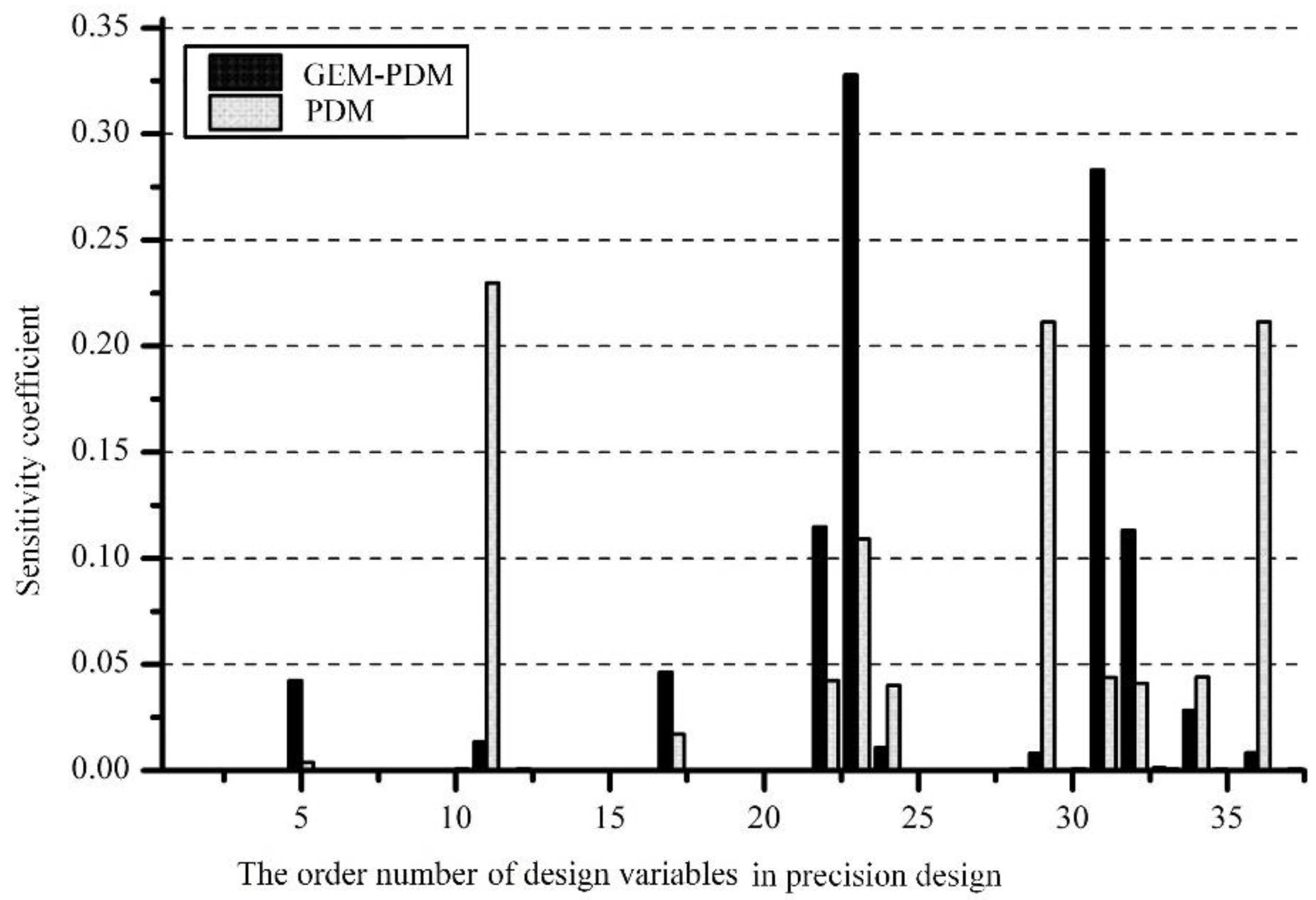
In order to verify the rationality of the gravity-induced error-modelling-based static precision design method (GEM-PDM) proposed in this paper, the static precision design method (PDM) for the machine tool based on the MBS kinematics [13] was used to obtain heavy-duty vertical precision results without considering the influence of the gravity deformation errors. The static precision results of the machining center were compared with the error budgeting results in this paper (Table 4), with the comparison results shown in Figure 7 and Table 6. At the same time, according to the sensitivity coefficient calculation method in [27], the influence of each error on the volumetric error Ev of the TCP was analyzed, as shown in Figure 8.
Combining Figure 7, Table 6 and Figure 8, it can be seen that due to the consideration of the influence of the structural deformation under gravity in the GEM-PDM, the errors of the X-, Z-, and W-axes in the precision allocation results of this paper were all larger than the gravity deformation of the structure itself. The difference provided a certain reference for the precision requirements of the manufacturing and machining of related components. In the error budgeting results obtained by PDM, some of the error values were smaller than the gravity deformation of the structure, and it needed to be adjusted through the whole machine assembly to meet the precision requirements, which undoubtedly increased the difficulty of the assembly. The increase of assembly adjustment links was enough to cause the forced deformation of the machine tool and the increased assembly stress, which was not conducive to the maintenance of the machine tool precision. Once the gravity deformation error was guaranteed by the error budget results, the geometric error caused by manufacturing was controlled as small as possible, or the big values of the error could make the volumetric error exceed the precision requirement boundaries. That is the reason why the volumetric error results calculated by the PDM were −0.0337 mm, −0.0157 mm and 0.040 mm, close to the given boundaries, and the improvements of the volumetric error by the GEM-PDM were 84.0%, 87.3% and 0.1%.
At the same time, among the machine tool errors budgeted by the two precision design methods, the higher sensitivity coefficients were mainly the angular errors and the squareness errors, that is, the volumetric error of the machine tool was more sensitive to the changes of these two types of errors. It also showed that these two types of errors had a relatively large influence on the volumetric error of the machine tool, and their controllability was poor. On the other hand, the sensitivity coefficients corresponding to the positioning error and the straightness error were relatively small and were basically negligible compared with the angular errors and the squareness errors. The errors with higher sensitivity coefficients were also mainly concentrated on the angular error of the crossbeam around the Y-direction and the three angular errors of the column, which was consistent with the previous conclusion on the optimal configuration of component stiffness.
It is noted that the stiffness coefficients and volume fraction of each component were selected as independent design variables. However, the structural stiffness should be correlated to the given volume fraction to some extent. To make the GEM-PDM more accurate and realistic for budgeting the error components of heavy-duty machine tools, the idea of topology optimization will be introduced to reveal the relationship between the element stiffness and volume fraction in the future work.
7. Conclusions
Due to the large size and large span of heavy-duty machine tools, the structural deformation error caused by gravity accounts for a large proportion of the static error, and the influence of gravity deformation must be considered in the precision design. This paper presented a precision design method for HDVMCs based on gravity deformation error modelling. The results of the optimization solution showed that the precision design method proposed in this paper could better provide reference values for the precision requirements of the manufacturing and machining of the machine tool components. After using the method proposed in this paper, the error design values of the X-, Z- and W-axes in the case machine tool were all larger than the gravity deformation of the structure itself, which was more suitable for the maintenance of the assembly and machine tool precision than the existing method. The improvement of the volumetric error compared with those by the PDM were 84.0%, 87.3% and 0.1%. Once the gravity deformation error was guaranteed by the error budget results, the geometric error caused by manufacturing was controlled as small as possible by the GEM-PDM to limit the volumetric error, meeting the precision design requirements.
Author Contributions
Conceptualization, H.W. and T.L.; methodology, H.W. and T.L.; validation, T.L.; investigation, H.W.; writing—original draft preparation, H.W. and X.S.; writing—review and editing, D.M. and T.W.; submission, D.M.; supervision, T.L. All authors have read and agreed to the published version of the manuscript.
Funding
This research received no external funding.
Data Availability Statement
Not applicable.
Conflicts of Interest
The authors declare no conflict of interest.
Nomenclature
| A | The cross-sectional area of the spatial beam element. |
| B | The body in the multibody system. |
| C | The structural compliance. |
| E | The elastic modulus. |
| Ev | The volumetric error of the theoretical forming point of the actual machine tool. |
| Evx | The component of the volumetric error in the X-direction (mm). |
| Evy | The component of the volumetric error in the Y-direction (mm). |
| Evz | The component of the volumetric error in the Z-direction (mm). |
| F | The external load vector. |
| Fzi | The external force along the Z-axis direction received by the ith node in the global coordinate system |
| fg1 | The relative cost function. |
| fg2 | The equalization objective function. |
| fg3 | The robust optimization objective function. |
| fd1 | The compliance objective function. |
| fd2 | The stiffness loss function. |
| g | The acceleration of gravity. |
| h | The hinge in the multibody system. |
| Iy | The moment of inertia of the cross section around the neutral axis parallel to the y-axis. |
| I′y | The moment of inertia of the cross-section of the optimized spatial beam element. |
| Iz | The moment of inertia of the cross section around the neutral axis parallel to the z-axis. |
| I′z | The torsional moment of inertia of the cross section of the optimized spatial beam element. |
| J | The torsional moment of inertia of the cross section. |
| J′ | The torsional moment of inertia of the cross section of the optimized spatial beam element. |
| K | The overall stiffness matrix of the structure. |
| Ke | The stiffness matrix of the spatial beam element in the local coordinate system. |
| kji (j = x, y, z) | The stiffness coefficient of the spatial beam element. |
| LEj (j = 1~5, 8~11) | The element length of the machine tool component represented by the jth element. |
| l | The element length. |
| Mj(i) (j = x, y, z) | The nodal moment of each node around the X-, Y-, Z-axes. |
| Myi | The external moment of the ith node around the Y-axis in the global coordinate system. |
| mE | The mass of the machine tool component represented by the element. |
| m′E | The mass of machine tool components represented by the optimized element. |
| n | The number of elements. |
| P | The overall nodal load vector. |
| Pactual | The actual position coordinate of the TCP. |
| Pe | The nodal load vector in the local coordinate system of the element. |
| Pideal | The actual position coordinate of the TCP. |
| Pi(i) (I = u, v, w) | The nodal force of each node along the X-, Y-, Z-directions. |
| Pt | The position coordinate vector Pt of the TCP in the tool coordinate system. |
| ptx, pty, ptz | The position coordinates of the TCP in the X-, Y-, Z-directions of the tool coordinate system. |
| q | The displacement vector of the structural node. |
| qe | The nodal displacement vector in the local coordinate system of the element. |
| R | The support reaction force vector. |
| Sxy, Sxz, Syz, Syz, Syz, Syz, Syz | The squareness error components between the axes denoted in the corresponding subscript. |
| Te | The transformation matrix of the element from the local coordinate system to the global coordinate system. |
| Tij | The ideal HTMs of position and orientation of Bj with respect to Bi. |
| Tijs | The ideal HTMs of position and orientation that come from static state. |
| Tijp | The ideal HTMs of position and orientation that come from motion state. |
| T′ij | The actual HTMs of position and orientation of Bj with respect to Bi under error conditions. |
| ΔTij | The HTMs with parameters of static error components. |
| U | The nodal displacement vector of the entire structure. |
| vfi | The optimized volume fraction of the ith element. |
| xi (i = 1, 2, …, 37) | The design variables in the precision design. |
| xiF | The part of the structural gravity deformation error in the static error design variable xi. |
| xiG | The geometric error caused by the manufacturing process in the static error design variable xi. |
| xsi | The normalized relative value of the design variable xi. |
| δx(x), δy(x), δz(x) | The linear error components of the X-axis along the X-, Y- and Z-directions. |
| δx(y), δy(y), δz(y) | The linear error components of the Y-axis along the X-, Y- and Z-directions. |
| δx(z), δy(z), δz(z) | The linear error components of the Z-axis along the X-, Y- and Z-directions. |
| δx(w), δy(w), δz(w) | The linear error components of the W-axis along the X-, Y- and Z-directions. |
| δx(γ), δy(γ), δz(γ) | The linear error components of the C-axis along the X-, Y- and Z-directions. |
| δz(x)M | The geometric error caused by manufacturing. |
| δz(x)F | The structural gravity deformation error. |
| εx(x), εy(x), εz(x) | The angular error components of the X-axis around the X-, Y- and Z-directions. |
| εx(y), εy(y), εz(y) | The angular error components of the Y-axis around the X-, Y- and Z-directions. |
| εx(z), εy(z), εz(z) | The angular error components of the Z-axis around the X-, Y- and Z-directions. |
| εx(w), εy(w), εz(w) | The angular error components of the W-axis around the X-, Y- and Z-z directions. |
| εx(γ), εy(γ), εz(γ) | The angular error components of the C-axis around the X-, Y- and Z-directions. |
| ω1, ω2 and ω3 | The weights of the objective functions. |
References
- Shen, H.; Fu, J.; He, Y.; Yao, X. On-line Asynchronous Compensation Methods for Static/Quasi-Static Error Implemented on CNC Machine Tools. Int. J. Mach. Tools Manuf. 2012, 60, 14–26. [Google Scholar] [CrossRef]
- Slocum, H. Precision Machine Design; Society of Manufacturing Engineers: Southfield, MI, USA, 1992. [Google Scholar]
- Kiridena, V.S.B.; Ferreira, P.M. Kinematic Modeling of Quasistatic Errors of Three-axis Machining Centers. Int. J. Mach. Tools Manuf. 1994, 34, 85–100. [Google Scholar] [CrossRef]
- Rahman, M.; Heikkala, J.; Lappalainen, K. Modeling, Measurement and Error Compensation of Multi-axis Machine Tools. Part I: Theory. Int. J. Mach. Tools Manuf. 2000, 40, 1535–1546. [Google Scholar] [CrossRef]
- Zhang, H.; Yang, J.; Zhang, Y.; Shen, J.; Wang, C. Measurement and Compensation for Volumetric Positioning Errors of CNC Machine Tools Considering Thermal Effect. Int. J. Adv. Manuf. Technol. 2011, 55, 275–283. [Google Scholar] [CrossRef]
- Li, Y.; Zhao, J.; Ji, S.J.; Wang, X. A New Error Compensation Method for a Four-Axis Horizontal Machine Tool. Key Eng. Mater. 2016, 679, 1–5. [Google Scholar] [CrossRef]
- Fu, G.; Fu, J.; Shen, H.; Yao, X.; Chen, Z. NC Codes Optimization for Geometric Error Compensation of Five-axis Machine Tools with One Novel Mathematical Model. Int. J. Adv. Manuf. Technol. 2015, 80, 1879–1894. [Google Scholar] [CrossRef]
- Fu, G.; Gong, H.; Fu, J.; Gao, H.; Deng, X. Geometric Error Contribution Modeling and Sensitivity Evaluating for Each Axis of Five-axis Machine Tools Based on POE Theory and Transforming Differential Changes Between Coordinate Frames. Int. J. Mach. Tools Manuf. 2019, 147, 103455. [Google Scholar] [CrossRef]
- Wu, C.; Fan, J.; Wang, Q.; Chen, D. Machining Accuracy Improvement of Non-orthogonal Five-axis Machine Tools by A New Iterative Compensation Methodology Based on the Relative Motion. Int. J. Mach. Tools Manuf. 2018, 124, 80–98. [Google Scholar] [CrossRef]
- Breitzke, A.; Wolfgang, H. Workshop-Suited Geometric Errors Identification of Three-Axis Machine Tools Using On-Machine Measurement for Long Term Precision Assurance. Precis. Eng. 2022, 75, 235–247. [Google Scholar] [CrossRef]
- Gu, J.; Agapiou, J. Assessment and Implementation of Global Offset Compensation Method. J. Manuf. Syst. 2018, 48, 38–44. [Google Scholar]
- Inigo, B.; Colinas-Armijo, N.; de Lacalle, L.N.L.; Aguirre, G. Digital Twin-Based Analysis of Volumetric Error Mapping Procedures. Precis. Eng. 2021, 72, 823–836. [Google Scholar] [CrossRef]
- Chen, G.; Sun, Y.; Lu, L.; Chen, W. A New Static Accuracy Design Method for Ultra-Precision Machine Tool Based on Global Optimisation and Error Sensitivity Analysis. Int. J. Nanomanufacturing 2016, 12, 167–180. [Google Scholar] [CrossRef]
- Chen, G.D.; Sun, Y.Z.; Zhang, F.H.; Lu, L.H.; Chen, W.Q.; Yu, N. Dynamic Accuracy Design Method of Ultra-precision Machine Tool. Chin. J. Mech. Eng. 2018, 31, 8. [Google Scholar] [CrossRef]
- Fan, J.; Tao, H.; Wu, C.; Pan, R.; Tang, Y.; Li, Z. Kinematic Errors Prediction for Multi-axis Machine Tools’ Guideways Based on Tolerance. Int. J. Adv. Manuf. Technol. 2018, 98, 1131–1144. [Google Scholar] [CrossRef]
- Wu, C.; Wang, Q.; Fan, J.; Pan, R. A Novel Prediction Method of Machining Accuracy for Machine Tools Based on Tolerance. Int. J. Adv. Manuf. Technol. 2020, 110, 629–653. [Google Scholar] [CrossRef]
- Xu, Y.; Zhang, L.; Wang, S.; Du, H.; Chai, B.; Hu, S.J. Active Precision Design for Complex Machine Tools: Methodology and Case Study. Int. J. Adv. Manuf. Technol. 2015, 80, 581–590. [Google Scholar] [CrossRef]
- Li, J.; Xie, F.; Liu, X.J. Geometric Error Modeling and Sensitivity Analysis of a Five-axis Machine Tool. Int. J. Adv. Manuf. Technol. 2016, 82, 2037–2051. [Google Scholar] [CrossRef]
- Li, H.; Li, Y.; Mou, W.; Hao, X.; Li, Z.; Jin, Y. Sculptured Surface-oriented Machining Error Synthesis Modeling for Five-axis Machine Tool Accuracy Design Optimization. Int. J. Adv. Manuf. Technol. 2016, 89, 3285–3298. [Google Scholar] [CrossRef]
- Zhang, Z.; Liu, Z.; Cheng, Q.; Qi, Y.; Cai, L. An Approach of Comprehensive Error Modeling and Accuracy Allocation for the Improvement of Reliability and Optimization of Cost of a Multi-axis NC Machine Tool. Int. J. Adv. Manuf. Technol. 2017, 89, 561–579. [Google Scholar] [CrossRef]
- Sahoo, A.K.; Rout, A.K.; Das, D.K. Response Surface and Artificial Neural Network Prediction Model and Optimization for Surface Roughness in Machining. Int. J. Ind. Eng. Comput. 2015, 6, 229–240. [Google Scholar] [CrossRef]
- Peng, F.; Yan, R.; Chen, W.; Yang, J.; Li, B. Anisotropic Force Ellipsoid Based Multi-axis Motion Optimization of Machine Tools. Chin. J. Mech. Eng. 2012, 25, 960–967. [Google Scholar] [CrossRef]
- Portman, V.T.; Shneor, Y.; Chapsky, V.S.; Shapiro, A. Form-shaping function theory expansion: Stiffness model of multi-axis machines. Int. J. Adv. Manuf. Technol. 2014, 76, 1063–1078. [Google Scholar] [CrossRef]
- Ma, J.; Lu, D.; Zhao, W. Assembly Errors Analysis of Linear Axis of CNC Machine Tool Considering Component Deformation. Int. J. Adv. Manuf. Technol. 2015, 86, 281–289. [Google Scholar] [CrossRef]
- Shi, X.; Liu, H.; Li, H.; Liu, C.; Tan, G. Comprehensive Error Measurement and Compensation Method for Equivalent Cutting Forces. Int. J. Adv. Manuf. Technol. 2016, 85, 149–156. [Google Scholar] [CrossRef]
- Shi, Y.; Zhao, X.; Zhang, H.; Nie, Y.; Zhang, D. A New Top-Down Design Method for The Stiffness of Precision Machine Tools. Int. J. Adv. Manuf. Technol. 2016, 83, 1887–1904. [Google Scholar] [CrossRef]
- Chen, G.; Liang, Y.; Sun, Y.; Chen, W.; Wang, B. Volumetric Error Modeling and Sensitivity Analysis for Designing a Five-Axis Ultra-Precision Machine Tool. Int. J. Adv. Manuf. Technol. 2013, 68, 2525–2534. [Google Scholar] [CrossRef]
Figure 1.
Flowchart of the heavy-duty machine tool precision design method based on gravity deformation modelling.
Figure 1.
Flowchart of the heavy-duty machine tool precision design method based on gravity deformation modelling.

Figure 2.
Schematic diagram of the structure of the HDVMC.
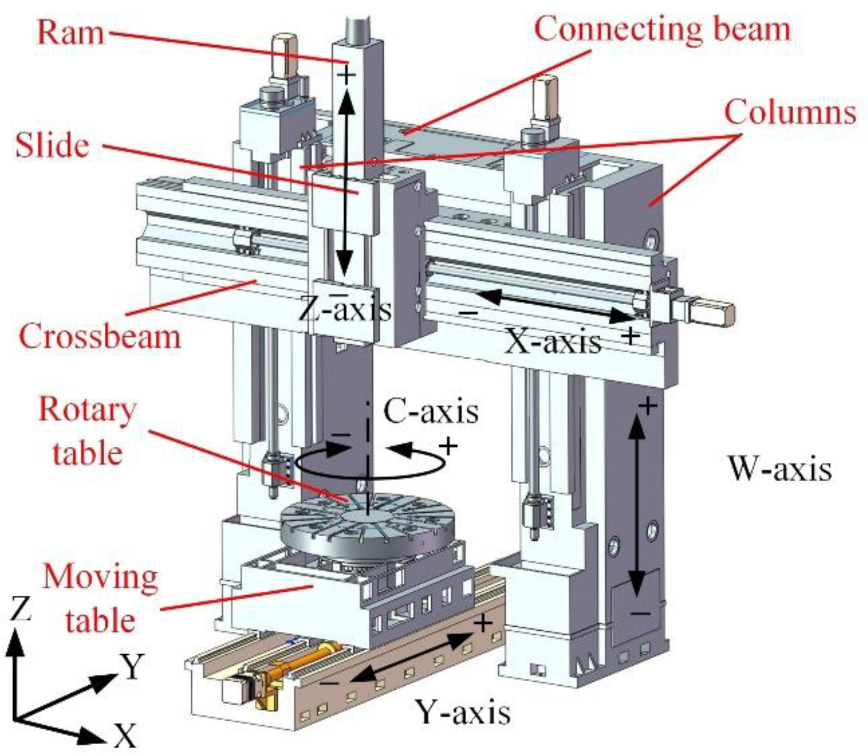
Figure 3.
The topological structure of the HDVMC.
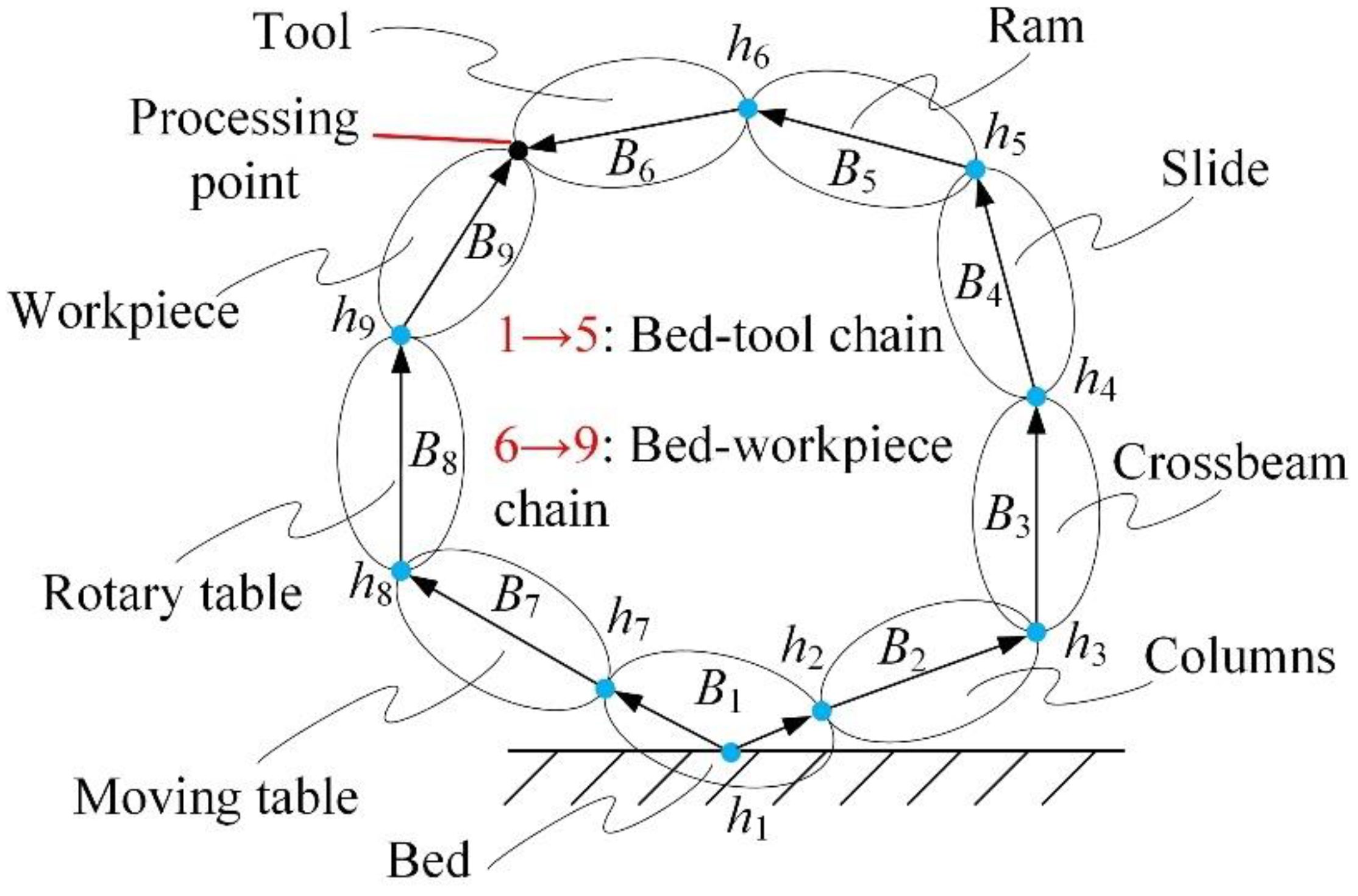
Figure 4.
Geometric features of kinematic with error existing between part Bi and Bj.

Figure 5.
Model of HDVMC based on spatial beam element. (a) Element node information and coordinate system definition. (b) Force analysis under gravity.
Figure 5.
Model of HDVMC based on spatial beam element. (a) Element node information and coordinate system definition. (b) Force analysis under gravity.

Figure 6.
Spatial beam element in local coordinate system.
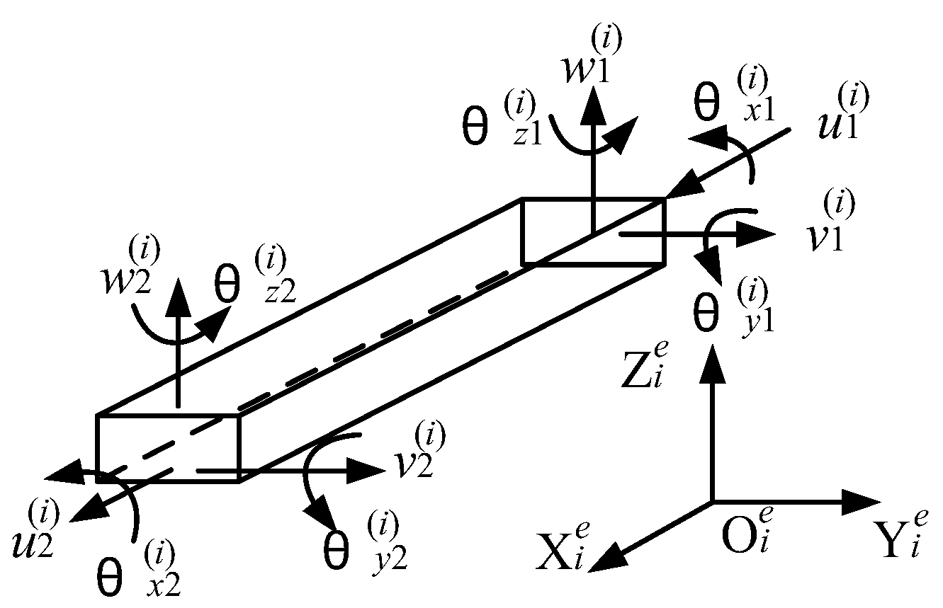
Figure 7.
Comparison of the results of precision assignment methods.

Figure 8.
Comparison of error sensitivity coefficient results for each precision allocation method.

Table 1.
Errors of each motion axis.
| Axis | Errors |
|---|---|
| X | δx(x), δy(x), δz(x), εx(x), εy(x), εz(x) |
| Y | δx(y), δy(y), δz(y), εx(y), εy(y), εz(y) |
| Z | δx(z), δy(z), δz(z), εx(z), εy(z), εz(z) |
| W | δx(w), δy(w), δz(w), εx(w), εy(w), εz(w) |
| C | δx(γ), δy(γ), δz(γ), εx(γ), εy(γ), εz(γ) |
Table 2.
Value ranges of design variables of static errors.
| Design Variable | Value Range | Design Variable | Value Range | Design Variable | Value Range |
|---|---|---|---|---|---|
| δx(x), (x1) | [0.006, 0.025] mm | δy(x), (x2) | [0.006, 0.03] mm | δz(x), (x3) | [0.006, 0.03] mm |
| εx(x), (x4) | [0.01, 0.04] mrad | εy(x), (x5) | [0.01, 0.04] mrad | εz(x), (x6) | [0.01, 0.04] mrad |
| δx(y), (x7) | [0.006, 0.03] mm | δy(y), (x8) | [0.006, 0.025] mm | δz(y), (x9) | [0.006, 0.03] mm |
| εx(y), (x10) | [0.01, 0.04] mrad | εy(y), (x11) | [0.01, 0.04] mrad | εz(y), (x12) | [0.01, 0.04] mrad |
| δx(z), (x13) | [0.006, 0.03] mm | δy(z), (x14) | [0.006, 0.03] mm | δz(z), (x15) | [0.006, 0.025] mm |
| εx(z), (x16) | [0.01, 0.04] mrad | εy(z), (x17) | [0.01, 0.04] mrad | εz(z), (x18) | [0.01, 0.04] mrad |
| δx(w), (x19) | [0.01, 0.03] mm | δy(w), (x20) | [0.01, 0.03] mm | δz(w), (x21) | [0.01, 0.025] mm |
| εx(w), (x22) | [0.01, 0.04] mrad | εy(w), (x23) | [0.01, 0.04] mrad | εz(w), (x24) | [0.01, 0.04] mrad |
| δx(γ), (x25) | [0.003, 0.01] mm | δy(γ), (x26) | [0.003, 0.01] mm | δz(γ), (x27) | [0.003, 0.01] mm |
| εx(γ), (x28) | [0.01, 0.04] mrad | εy(γ), (x29) | [0.01, 0.04] mrad | εz(γ), (x30) | [0.01, 0.04] mrad |
| Sxw, (x31) | [0.01, 0.04] mrad | Syw, (x32) | [0.01, 0.04] mrad | Sxy, (x33) | [0.01, 0.03] mrad |
| Sxz, (x34) | [0.01, 0.06] mrad | Syz, (x35) | [0.01, 0.06] mrad | Sxc, (x36) | [0.01, 0.02] mrad |
| Syc, (x37) | [0.01, 0.02] mrad |
Table 3.
Value range of structural design variables.
| Design Variable | Variable Meaning | Value Range | Design Variable | Variable Meaning | Value Range |
|---|---|---|---|---|---|
| x38 | Section width of connecting beam | [0.7, 1] m | x47 | X-directional stiffness coefficient of column | [0.2, 1] |
| x39 | Section height of connecting beam | [0.9, 1.2] m | x48 | Y-directional stiffness coefficient of column | [0.2, 1] |
| x40 | Volume factor of connecting beam | [0.25, 1] | x49 | Z-directional stiffness coefficient of column | [0.2, 1] |
| x41 | Z-directional stiffness coefficient of connecting beam | [0.2, 1] | x50 | Section width of crossbeam | [0.67, 0.8] m |
| x42 | Y-directional stiffness coefficient of connecting beam | [0.2, 1] | x51 | Section height of crossbeam | [1, 1.2] m |
| x43 | X-directional stiffness coefficient of connecting beam | [0.2, 1] | x52 | Volume factor of crossbeam | [0.45, 1] |
| x44 | Section width of column | [0.6, 0.8] m | x53 | X-directional stiffness coefficient of crossbeam | [0.2, 1] |
| x45 | Section height of column | [1, 1.25] m | x54 | Y-directional stiffness coefficient of crossbeam | [0.2, 1] |
| x46 | Volume factor of column | [0.25, 1] | x55 | Z-directional stiffness coefficient of crossbeam | [0.2, 1] |
Table 4.
The optimal solution of precision distribution obtained by genetic algorithm optimization.
| Design Variable | Optimized Value | Design Variable | Optimized Value | Design Variable | Optimized Value |
|---|---|---|---|---|---|
| δx(x), (x1) | 0.017 mm | δy(x), (x2) | 0.009 mm | δz(x), (x3) | 0.011 mm |
| εx(x), (x4) | 0.028 mrad | εy(x), (x5) | 0.022 mrad | εz(x), (x6) | 0.016 mrad |
| δx(y), (x7) | 0.013 mm | δy(y), (x8) | 0.018 mm | δz(y), (x9) | 0.027 mm |
| εx(y), (x10) | 0.022 mrad | εy(y), (x11) | 0.012 mrad | εz(y), (x12) | 0.04 mrad |
| δx(z), (x13) | 0.014 mm | δy(z), (x14) | 0.027 mm | δz(z), (x15) | 0.009 mm |
| εx(z), (x16) | 0.038 mrad | εy(z), (x17) | 0.011 mrad | εz(z), (x18) | 0.04 mrad |
| δx(w), (x19) | 0.029 mm | δy(w), (x20) | 0.03 mm | δz(w), (x21) | 0.014 mm |
| εx(w), (x22) | 0.04 mrad | εy(w), (x23) | 0.027 mrad | εz(w), (x24) | 0.035 mrad |
| δx(γ), (x25) | 0.013 mm | δy(γ), (x26) | 0.008 mm | δz(γ), (x27) | 0.017 mm |
| εx(γ), (x28) | 0.017 mrad | εy(γ), (x29) | 0.017 mrad | εz(γ), (x30) | 0.024 mrad |
| Sxw, (x31) | 0.026 mrad | Syw, (x32) | 0.039 mrad | Sxy, (x33) | 0.021 mrad |
| Sxz, (x34) | 0.017 mrad | Syz, (x35) | 0.054 mrad | Sxc, (x36) | 0.012 mrad |
| Syc, (x37) | 0.02 mrad |
Table 5.
The optimal solution of stiffness distribution obtained by genetic algorithm optimization.
| Design Variable | Optimized Value | Design Variable | Optimized Value |
|---|---|---|---|
| x38 | 0.75 m | x47 | 0.32 |
| x39 | 0.91 m | x48 | 0.62 |
| x40 | 0.26 | x49 | 0.2 |
| x41 | 0.2 | x50 | 0.7 m |
| x42 | 0.2 | x51 | 1.2 m |
| x43 | 0.21 | x52 | 0.46 |
| x44 | 0.78 m | x53 | 0.57 |
| x45 | 1.24 m | x54 | 0.21 |
| x46 | 0.27 | x55 | 0.37 |
Table 6.
Comparison of the error budgeting results by PDM and GEM-PDM.
| Item | GEM-PDM | PDM |
|---|---|---|
| Evx (mm) | −0.0054 | −0.0337 |
| Evx (mm) | −0.0020 | −0.0157 |
| Evx (mm) | 0.0396 | 0.040 |
Publisher’s Note: MDPI stays neutral with regard to jurisdictional claims in published maps and institutional affiliations. |
© 2022 by the authors. Licensee MDPI, Basel, Switzerland. This article is an open access article distributed under the terms and conditions of the Creative Commons Attribution (CC BY) license (https://creativecommons.org/licenses/by/4.0/).
Share and Cite
MDPI and ACS Style
Wang, H.; Li, T.; Sun, X.; Mynors, D.; Wu, T. Optimal Design Method for Static Precision of Heavy-Duty Vertical Machining Center Based on Gravity Deformation Error Modelling. Processes 2022, 10, 1930. https://doi.org/10.3390/pr10101930
AMA Style
Wang H, Li T, Sun X, Mynors D, Wu T. Optimal Design Method for Static Precision of Heavy-Duty Vertical Machining Center Based on Gravity Deformation Error Modelling. Processes. 2022; 10(10):1930. https://doi.org/10.3390/pr10101930
Chicago/Turabian StyleWang, Han, Tianjian Li, Xizhi Sun, Diane Mynors, and Tao Wu. 2022. "Optimal Design Method for Static Precision of Heavy-Duty Vertical Machining Center Based on Gravity Deformation Error Modelling" Processes 10, no. 10: 1930. https://doi.org/10.3390/pr10101930
Note that from the first issue of 2016, this journal uses article numbers instead of page numbers. See further details here.