Time-Series Monitoring of Transgenic Maize Seedlings Phenotyping Exhibiting Glyphosate Tolerance

Abstract

Glyphosate is a widely used nonselective herbicide. Probing the glyphosate tolerance mechanism is necessary for the screening and development of resistant cultivars. In this study, a hyperspectral image was used to develop a more robust leaf chlorophyll content (LCC) prediction model based on different datasets to finally analyze the response of LCC to glyphosate-stress. Chlorophyll a fluorescence (ChlF) was used to dynamically monitor the photosynthetic physiological response of transgenic glyphosate-resistant and wild glyphosate-sensitive maize seedlings and applying chemometrics methods to extract time-series features to screen resistant cultivars. Six days after glyphosate treatment, glyphosate-sensitive seedlings exhibited significant changes in leaf reflection and photosynthetic activity. By updating source domain and transfer component analysis, LCC prediction model performance was improved effectively (the coefficient of determination value increased from 0.65 to 0.84). Based on the predicted LCC and ChlF data, glyphosate-sensitive plants are too fragile to protect themselves from glyphosate stress, while glyphosate-resistant plants were able to maintain normal photosynthetic physiological activity. JIP-test parameters, φ_E0, V_J, ψ_E0, and M₀, were used to indicate the degree of plant damage caused by glyphosate. This study constructed a transferable model for LCC monitoring to finally evaluate glyphosate tolerance in a time-series manner and verified the feasibility of ChlF in screening glyphosate-resistant cultivars.

1. Introduction

Glyphosate is one of the most popular herbicides in grass control with non-selective and broad-spectrum characteristics [1,2]. Glyphosate acts on all green plants, including crops. Consequently, the use of glyphosate is limited in time and space. On the other hand, under glyphosate stress, weeds are more prone to genetic mutations that show tolerance to glyphosate than crops [1,3], which provides a new way to acquire glyphosate-resistant varieties. With the rapid development of genetic engineering and genomics, the development and popularization of superior varieties can be achieved. Glyphosate has become more ubiquitously used in agriculture since the introduction of glyphosate-resistant cultivars.

The analysis of the difference between resistant and sensitive cultivars is helpful to probe the glyphosate tolerance mechanism and promote the creation of new cultivars. The traditional detection method of herbicide resistance is to observe seedlings’ growing status with the naked eye after spraying the herbicide on them. Generally speaking, it takes 12 days from the application of stress to the determination of herbicide injury level and final resistance identification [4], which is time-consuming, subjective, and inefficient. Professional technologies, such as PCR, often require expensive experimental equipment and professional operating knowledge, which limits the convenience and real-time detection. Therefore, building an expeditious and accurate detection method would be an invaluable tool for excellent cultivar development.

Furthermore, chlorophyll content provides a good access to evaluate the level of tolerance to herbicide stress of crops. The photosynthetic pigment is located in the membrane of plant thylakoids that captures and transfers light energy or causes initial photochemical reactions. The physiological requirements and material accumulation capacity of plants can be uncovered according to changes in pigment content [5]. Hence, pigment content in leaves is one of the most frequently used to evaluate plant nutrition, health status, and physiological response to environmental conditions including various stresses [6]. Currently, the use of a spectrophotometer is still a standard method for the determination of photosynthetic pigment content, which is not only destructive but also makes it difficult to meet the requirements of modern agriculture due to its lag. The emerging hyperspectral technology has yielded a positive foundation in the evaluation of pigment, usually based on machine learning and chemometrics, but the method is still in the development stage. The leaf chlorophyll content prediction model is not suitable for other sample sets, and there are few studies that have linked prediction values to actual experimental phenomena to illustrate the stress response, such as the mechanism of action of glyphosate stress in plants.

As another technique for indirectly sensing plant pigment statues, rapid Chl a fluorescence (ChlF) can obtain enough information about the structure and function of photosystem II (PSII) in just a few seconds and detect a stress response before plants exhibit visible signs or other detection methods, such as the measurements of gas exchange or changes in pigment [7,8]. In recent years, ChlF has been ubiquitously adopted to assess the direct effects of biotic and abiotic stresses, such as high temperature [9], drought and heavy metals [10], and ultimately for tolerant cultivar selection [11,12]. Generally speaking, under most stresses, two target sites will be affected in plant chloroplasts. The one is the electron transport chain, which is related to the utilization of absorbed light energy. The other one is the synthesis of Chl and carotenoids, which is associated with light-harvesting complex (LHC) and the antenna of the photosynthetic reaction center [8]. The above changes can be captured by the OJIP curve and JIP-test parameters. The OJIP curve contains the relationship between the light reaction stage and PSII fluorescence [13], and JIP-test parameters include the absorption and trapping of energy and electron transport information.

Apart from the above-mentioned, to our knowledge, there are few studies that applying hyperspectral technology and prompt ChlF transient to dynamically monitor glyphosate tolerance in different maize genotypes in time-series. This study will provide an expeditious and accurate phenotypic analysis method for screening resistant cultivars and has the potential to advance crop breeding. In turn, the gap between plant phenotype and transgenic technology pushes us to explore the response and characteristic fingerprint of different resistant varieties under glyphosate stress. Therefore, this study aims to (1) develop a more robust leaf chlorophyll content (LCC) prediction model; (2) explore the feasibility of rapid ChlF transience to dynamically monitor the photosynthetic physiological response of different resistant maize varieties under glyphosate stress; (3) analyze and uncover the effects of glyphosate-stress on plant photosynthetic characteristics; and (4) select characteristic fingerprints to evaluate the tolerance of glyphosate. The results of this study will provide a new tool for the identification of excellent traits which may possibly improve the efficiency of crop breeding in the long run.

2. Materials and Methods

2.1. Plant Materials and Experimental Setup

The accession of maize, including the glyphosate-sensitive wild type (recorded as GS) and glyphosate-resistant type (recorded as GR), were provided by the Institute of Insect Sciences, Zhejiang University, Hangzhou, China. The glyphosate-tolerance of GR was acquired by the expression of a mutant 5-enolpyruvylshikimate-3-phosphate synthase enzyme (the specific protocol was described in previous research [14]).

Three individual experiments (Experiments 1, 2, and 3) were conducted in the same greenhouse in August, November, and December 2021, respectively. Parameter settings followed the published research [15] with minor modifications. In each experiment, the temperature and photoperiod of day/night were 28/26 °C and 11/13 h, respectively; the average relative humidity was adjusted to 55%; and the maximum photosynthetically active radiation was about 1400 μmol (photons) m⁻² s⁻¹. Specifically, maize seeds were sown in seeding clods at one per pot, and on the 9th day post-sowing (two-leaf stage, the second leaf was fully expanded but the third leaf had just emerged), plants of similar growing state were picked and transplanted into a plastic bucket with drainage holes, and each pot was only occupied by one plant. When plants grew to the three-leaf stage (the third leaf was fully expanded but the fourth leaf had just emerged) on the 15th day post-sowing, part of plant was subjected to glyphosate (Roundup Original^®, Monsanto Company, St. Louis, MO, USA) as treatment at the recommended dose by using a portable sprayer, and the others were sprayed with water as control. Therefore, there were four groups (two varieties × two treatments) in our research, namely RT, RW, ST, and SW (“R” stands for “glyphosate-resistant”, “S” stands for “glyphosate-sensitive”, “T” stands for “with glyphosate”, and “W” stands for “with water”). ChlF and hyperspectral measurement were performed at 2, 4, 6, and 8 days after treatment (DAT) to monitor and assess photosynthetic apparatus in time scale. No less than four plants of each group at each sampling point were randomly selected, and all the measurements were conducted on the 1st, 2nd, and 3rd leaves (recorded as L1, L2, and L3 from the bottom to top, respectively) of maize plants. The details of each independent experiment were shown in Figure 1.

2.2. Acquisition of Hyperspectral Imaging In Vivo

The hyperspectral image acquisition of fresh maize seedlings was conducted by a line-scan hyperspectral imaging system in the Vis-NIR range (380–1030 nm), which was described in our previous study at length [16]. In the pre-experiment, in order to guarantee hyperspectral images sharpness and without distortion, we adjusted the camera exposure time, the intensity of the line light source, the distance between the camera lens and the moving plate, and the speed of the conveyer belt to 70 ms, 240, 390 mm, and 5 mm/s, respectively. Over the hyperspectral image acquisition, the maize seedlings’ growth morphology was kept as naturally as possible, and they were placed flat on a black plate without overlapping between leaves.

The original hyperspectral images of the maize seedlings were corrected by the black and white reference images, which were obtained under the same system parameters as samples. Prior to estimating LCC, image segmentation must be applied to identify the entire area of each expanding leaf as the region of interest (ROI). Hence, each plant had three ROIs corresponding to three leaf positions (L1, L2, and L3). For each ROI, after the head-to-tail spectra bands with high noise were discarded, the spectral reflectance of all pixels at 450–902 nm were averaged to represent the corresponding leaf.

2.3. Measurement of ChlF In Vivo

The measurements of ChlF transient curves were completed using a continuous excitation chlorophyll fluorimeter (Handy-PEA, Plant Efficiency Analyzer, Hansatech Instruments Ltd., Norfolk, United Kingdom) at room temperature (ca. 26 °C) from 11:30 to 15:00. After hyperspectral image acquisition, three clips were immediately placed on the basal, central, and top positions of the adaxial side of each leaf, respectively, for a 25 minutes’ dark adaption to allow all PSII reaction centers (RCs) open (Q_A⁻ gets reoxidized), and ferredoxin-NADP⁺-reductase to become inactive. Then a polyphasic ChlF transient curve was able to be obtained through the illumination of a saturating light excited by an array of three ultra-bright red LED (3000 μmol·m⁻²·s⁻¹; peak wavelength at 650 nm). The typical OJIP transient was recorded during the 1 s period that included four steps O (at 20 μs), J (at 2 ms), I (at 30 ms), and P (peak). Once kinetic ChlF rise curve was obtained, all leaves were stored in zip-lock bags at −80 °C until LCC measurement.

2.4. A Brief Information of OJIP Fluorescence Transient and JIP-Test

OJIP fluorescence transient curve reflects the sequential events with four general steps [17]. O-step refers to the initial fluorescence level (F₀). P-step is the peak level with all RCs closed. J-step and I-step are transitory steady-states of Q_A⁻ concentration, as the slope of curve at these steps are zero, which means that the reduction rate of Q_A is equal to the oxidation rate of Q_A⁻. Between the two adjacent steps, denoted as a phase, it reflects different photochemical stages. The OJ-phase is mostly driven by primary photochemistry, almost only single-turnover (Q_A to Q_A⁻) events are going on. Because Q_B could not accept an electron from Q_A⁻ in time to reoxidized it (the electron transport time is ~250 ps from pheo⁻ to Q_A, but 0.1~0.6 ms from Q_A⁻ to Q_B), resulting in a large accumulation of Q_A, and causing the fluorescence intensity to increase. JI-phase mainly refers to the reflection of the intersystem electron carriers Q_B, plastoquinone (PQ), and cytochrome (Cyt b6/f). IP-phase refers to PSI acceptor side [18].

On the basic of OJIP trajectory and the theory of “energy flow” across thylakoid membranes, quantitative method so-called JIP-test, is used to explore detailed information of PSII status and function, including RCs, light-harvesting antenna, and both the donor and acceptor sides. All the JIP-test parameters can be divided into four groups in general: (1) basic measured and calculated values; (2) quantum yield and probabilities/efficiencies; (3) energy flux; and (4) performance indices. Of these, the parameters used in this study are listed in detail in

Table 1. Glossary, formula, and explanation of terms used in the JIP-test for analysis OJIP fluorescence transient curve emitted by dark-adapted photosynthetic samples in this study. Subscript “0” (or “o”) indicates that the parameter refers to the onset of illumination. Symbol “F” stands for “fluorescence”, meaning fluorescence intensity.

Formula and Terms	Explanation
Parameters extracted from the recorded fluorescence transient OJIP
F0 ≈ F20μs	Fluorescence when all PSII RCs are open
FM (=FP)	Maximal fluorescence when all PSII RCs are closed
FL ≈ F100μs	Fluorescence at 100 μs
FK ≈ F300μs	Fluorescence at 300 μs
FJ = F2ms	Fluorescence at the J-step (2 ms) of OJIP
FI = F30ms	Fluorescence at the I-step (30 ms) of OJIP
$t_{F_M}$	Time (in ms) to reach the maximal fluorescence FM
Parameters derived from extracted fluorescence data
Area	Total complementary area between fluorescence induction curve and F = FM
Sm	Area/tFM
Fv = FM − F0	Maximal variable fluorescence
Fv/F0	Efficiency of the water-splitting complex on the donor side of PSII
Vt = (Ft − F0)/(FM − F0)	Relative variable fluorescence at time t (normalization on FM − F0)
W(YZ), t = (Ft − FY)/(FZ − FY)	Different types of relative variable fluorescence at time t, with (FZ − FY) standing for (F300µs − F0) or (FJ − F0) or (FI − FJ) or (FI − F0) or (FP − FI)
M0 = [(△F/△t)0]/(FM − F0) = 4 × (F300µs − F20µs)/(FM − F0) = 4 × (V300µs − V20µs)	Approximated initial slope (in ms−1) of the fluorescence transient normalized on the maximal variable fluorescence FM − F0; equivalently, initial slope (20 to 300 µs; in ms−1) of the Vt = f(t) kinetics
Specific energy fluxes per QA− reducing PSII reaction center (RC) and per cross section (CS) at t = 0
ABS/RC = M0·(1/VJ)/(1 − F0/Fm)	Absorption flux per reaction center (RC) by exciting PSII antenna Chlorophyll molecules
TR0/RC = M0·(1/VJ)	Trapping energy flux for QA reduction at PSII reaction center (RC)
ET0/RC = M0·(1/VJ)·(1 − VJ)	Electron transport flux per active reaction center (RC)
RE0/RC = M0·(1/VJ)·(1 − VI)	Electron flux reducing end electron acceptors at the photosystem I (PSI) acceptor side per reaction center (RC)
ABS/CS0 ≈ F0	Absorption flux per cross section (CS) by exciting PSII antenna Chlorophyll molecules
TR0/CS0 = φP0·F0	Trapping energy flux for QA reduction per cross section (CS)
ET0/CS0 = φE0·F0	Electron transport flux per cross section (CS)
RE0/CS0 = φE0·φR0·F0	Electron flux reducing end electron acceptors at the photosystem I (PSI) acceptor side per cross section (CS)
Quantum yields and probabilities/efficiencies
φP0 = TR0/ABS = 1 − F0/Fm	Maximum quantum yield of Photosystem II primary photochemistry in the dark-adapted state
ψE0 = ET0/TR0 = 1 − VJ	Probability that a trapped exciton moves an electron into the electron chain beyond QA−
φE0 = ET0/ABS = (1 − F0/Fm)·(1 − VJ)	Quantum yield for electron transport
δR0 = RE0/ET0 = (1 − VI)/(1 − VJ)	Efficiency/probability of electron transfer from the PQ pool, beyond QA− and reduction of end electron acceptors in PSI
φR0 = RE0/ABS = (1 − F0/Fm)·(1 − VI)	Quantum yield for the reduction of the end acceptors of PSI per photon absorbed
Other biophysical parameters
γRC = RC/(ABS + RC)	Probability that a PSII Chlorophyll a molecule functions as RC
RC/CS0 = φP0 − (VJ/M0)·(ABS/CS)	Density of RCs (QA− reducing PSII reactive centers)
Performance indices
PIABS = (RC/ABS)·(φP0/(1 − φP0))·(ψE0/(1 − ψE0))	Performance index for energy conservation from photos absorbed by PSII until the reduction of intersystem electron acceptors

[19] with minor modifications.

2.5. Measurement of Leaf Chlorophyll Content

The measurement of LCC was followed by the traditional protocol with minor modification [20]. Similar to ChlF acquisition, three discs of 5 mm diameter were taken from the basal, central, and top positions of each leaf, respectively. LCC in discs were extracted entirely after soaking in 4 mL ethanol and water (95% (v/v)) for 48 h in dark environment. Then pigment content was measured by spectrophotometry (Epoch, BioTek Instruments Winooski, VT, USA). Finally, according to the standard curves and the absorbance of light at 470, 649, and 665 nm, Chlorophyll content was calculated. The basal, central, and top positions of each leaf were averaged as the corresponding phenotypic traits of each leaf.

2.6. Data Analysis and Model Development

In this study, based on spectral reflectance datasets from three independent experiments (Experiments 1–3) conducted at different times, we explored model transferability across different datasets and evaluated the performance of two transfer strategies. In order to overcome experiment condition diversity and improve the robustness of LCC estimation model, the following two strategies (Figure 1) were used. Strategy_1, updating the source domain, was to add a portion of the samples (≤50%) of the target domain to the source domain, which were selected by the Kennard–Stone (KS) algorithm. Strategy_2, the transfer component analysis (TCA), was to narrow the data distribution difference between the source domain and target domain. The above strategies could be regarded as the preprocessing step. To build an LCC estimation model, the commonly used machine learning algorithms, random forest (RF) and support vector machine (SVM), were used. For the RF regression model, the range of the minimum number of observations per tree leaf was set from 5 to 25 with a step of 5, the range of the number of decision trees was set from 100 to 300 with a step of 50, and the optimal value was determined by 10-fold cross validation. For SVM regression model, the epsilon-SVR algorithm was used. The epsilon in loss function (p) was set to 0.1, and the particle swarm optimization method was applied to optimize model parameters (‘g’: gamma, ranges from 0.1 to 100, ‘c’: cost, ranges from 0.01 to 1000). The performances of prediction models were quantified by the coefficient of determination (R²) and the root of mean square error (RMSE). The above algorithms were conducted on Matlab 2016a (The MathWorks, Natick, MA, USA).

With glyphosate applied, plants exhibited complex physiological responses, which subtly varied depending on plant tolerance degree and stress time. To obtain a general view of the dataset and understand the resistant mechanism of GR and GS on the time scale, principal component analysis (PCA) was performed to visualize time-series phenotypic data and further discussion intuitively. An analysis of variance (ANOVA) was then applied to quantify the differences of JIP-test parameters between four groups on 2, 4, 6, and 8 DAT. Significant differences were evaluated at a significance level (P) of 0.05 and Holm–Bonferroni test was used as the post hoc test. Moreover, PCA replaced the original variables with fewer new variables through linear combination, which retained as much information as possible from the original variable. Hence, according to JIP-test parameters’ absolute value, PCA-loadings was applied to select optimal features on each sampling point. Then, the Ward.D linkage clustering method was used to validate the performance of the selected features. The above methods were implemented on Origin 2021b (OriginLab Corporation, Northampton, MA, USA).

3. Results

3.1. Establishment of LCC Prediction Model Based on Spectral Reflectance

Two machine learning algorithms and two transfer strategies were employed to predict LCC based on the multi-temporal spectral reflectance, and the results were shown in Table S1. In this section, the spectral datasets of Experiments 1 and 2 were set as source domain to establish prediction model to estimate LCC of target domain Experiment 3. The better prediction result was based on the SVM regression model and obtained R²_p was 0.65 and RMSE_p was 4.94 μg cm⁻². When added new samples from target domain (strategy_1), there was an increasing tendency of R²_p. In the SVM-based algorithm, the range of R²_p and RMSE_p was 0.70~0.81 and 4.39~4.80 μg⸱cm⁻², respectively. In the RF-based algorithm, the range of R²_p and RMSE_p was 0.57~0.62 and 6.11~6.42 μg⸱cm⁻², respectively. Therefore, the best estimation result was obtained on the SVM regression model when adding 144 samples from target domain to source domain (R²_p = 0.81 and RMSE_p = 4.42 μg⸱cm⁻²). Considering the change of data distribution caused by source domain update, TCA (strategy_2) was applied to narrow the difference of data distribution between source domain and target domain. The estimation results (Table S1) were further improved, which was embodied in the increasing tendency of R²_p and the decreasing of RMSE. The above indicated that both source domain update and applying TCA algorithm could narrow the data distribution difference between source domain and target domain and improve prediction performance. The results were consistent with previous literature [21,22,23]. By comparing the results of different strategies, TCA_SVM regression model with 144 new samples exhibited the best results (R²_p = 0.84, and RMSE_p = 4.03 μg⸱cm⁻²), and the predicted and measured LCC were plotted in scatterplot in Figure 2.

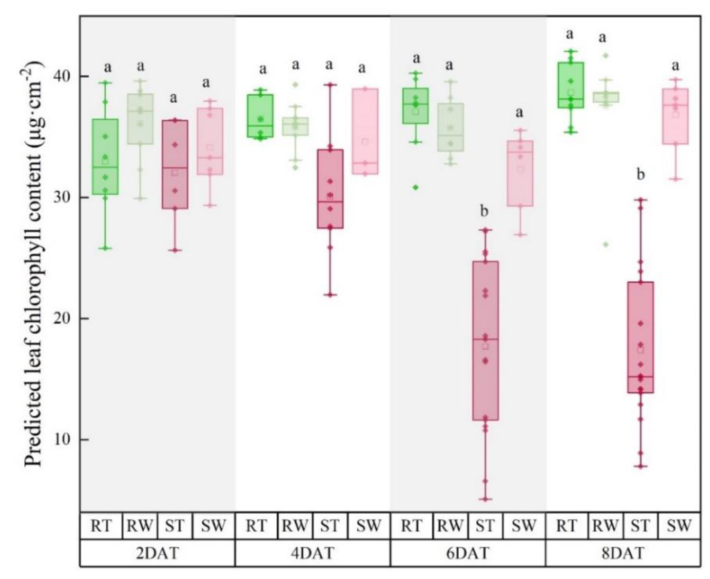
3.2. Effect of Glyphosate Stress on Pigment Content within Leaves of Maize Seedlings

Based on LCC predicted by the model with the best performance, its ANOVA result was shown in Figure 3. Although RT plants’ LCC decreased on 2 DAT, there was no significant difference seen between RT and RW plants throughout the trial. However, ST plants revealed notable lower LCC when compared to SW on 4 DAT, and this tendency was more obvious on 6 and 8 DAT. This result was similar to previous studies [16,24], which indicated that the two transfer strategies can improve the transferability of model and are expected to estimate LCC of samples from other datasets accurately.

3.3. OJIP Transient Captures the Difference Responses to Glyphosate Stress

In Experiment 3, the OJIP transient curves of all four groups presented a typical polyphasic O-J-I-P shape on a logarithmic time scale at the early stage of treatment (Figure 4). The OJIP curves of RW and SW plants were basically the same at four sampling points. This indicated that there was no significant difference in photosynthetic response between the two cultivars. The spraying with glyphosate did not cause a change in F₀ but led to a change in fluorescence intensity at J, I, and P steps before the plants died. Regardless of cultivar, the P-step was the most sensitive to glyphosate among the four steps in OJIP curves. The fluorescence intensity at P-step (F_M) decreased significantly in both cultivars at 2 DAT. Interestingly, the fluorescence intensity difference between RT and RW decreased from 2 DAT progressively, and at 6 DAT, the difference had almost disappeared, which suggested GR plants returned to a normal photosynthetic state at 6 DAT. However, the OJIP curve trend of ST was significantly different from SW at 6 DAT without a recovery sign. Therefore, under glyphosate stress, the difference of OJIP curves between GR and GS became obvious with time both in fluorescence intensity and curve morphology, which indicated the feasibility of the ChlF transient curve in screening glyphosate-resistant cultivars. Similar results were observed in Experiments 1 and 2 (Figure S1). Thus, the results of Experiment 3 were mainly presented and analyzed in the following sections.

To further visualize the information hidden in the raw OJIP transient curves, a semiquantitative analysis of normalization [25] was applied for the better depiction of respond difference between GR and GS. Normalization and corresponding subtractions were carried out in the OK, OJ, OI, and IP-phase, respectively. The fluorescence rise kinetics was normalized between O-step (20 μs) and K-step (300 μs), as W_OK = (F_t − F₀)/(F_K − F₀), then the difference kinetics (ΔW_OK = W_{OK (treatment)} − W_{OK (control)}) were plotted in the linear time scale (Figure 5A). Between O-step and K-step, a hidden L-band (~100 μs) could be observed by such a subtraction. As researchers reported [18], a negative L-band was the signal of good energetic connectivity or the grouping of PSII units, while a positive L-band was caused by stress. Therefore, Figure 5A shows that the L-band of ST plants could be observed clearly, and the value of ∆W_OK at L-band increased with time. On the other hand, RT plants retained a negative L-band with slight fluctuation from 2 DAT to 8 DAT. In the same way, in order to explore whether the application of glyphosate lead to the emergence of K-band, raw fluorescence data were double normalized by F₀ (20 μs) and F_J (2 ms), as W_OJ = (F_t − F₀)/(F_J − F₀) and the difference between treatment and control (ΔW_OJ = W_{OJ (treatment)} − W_{OJ (control)}) was calculated and plotted on a logarithmic time scale (Figure 5B). The trend of curves was similar to Figure 5A, K-band (~300 μs) in ST plants was elicited at 6 DAT and up to maximum at 8 DAT. However, RT plants were still below the zero level at all sampling points. This indicated that glyphosate affected the inactivation of the oxygen-evolving complex (OEC) centers in sensitive cultivars. Of course, this effect would become more serious over time. Moreover, IP-phase was evaluated by two frequently used normalization procedures to obtain information on PSI acceptor side. As shown in Figure 5C, double normalization between O-step (20 μs) and I-step (30 ms), as W_OI = (F_t − F₀)/(F_I − F₀), was plotted in the linear time scale (only W_OI > 1 was shown). In Figure 5D, double normalization between I-step (30 ms) and the peak of fluorescence intensity (~500 ms), as W_IP = (F_t − F₀)/(F_P − F_I) was plotted in its linear time scale. Therefore, we were able to find changes between different cultivars/treatment/DAT from W_OI = f(t) and W_IP = f(t). The maximal amplitude of the W_OI curve was positively related to the relative size of the end electron acceptors pool at PSI acceptor side. From Figure 5C it can be seen that RT plants had higher amplitude than RW plants, while the opposite phenomenon appeared in GS plants, which might be related to the resistance mechanism of the glyphosate-resistant cultivar. A comparison of W_IP = f(t) could provide insight into the overall reduction rate of the end electron acceptors pool at PSI acceptor side, which rules out possible effects on pool size. Here it shown that glyphosate resulted in a decreased rate only in ST plants (Figure 5D). Generally, the half-time, corresponding to W_IP = 0.5, was negatively correlated with electron transport rate. Thus, from the analysis of the IP-phase, it was concluded that the glyphosate introduced a greater size of the end electron acceptors pool without a change in electron transport rate for GR plants, while the smaller size of the end electron acceptors pool and lower electron transport rate for GS plants.

3.4. Effect of Glyphosate Stress on PSII and PSI by JIP-Test

As a quantitative method, on the basis of several assumptions and approximations [18], the JIP-test plays an important role in the translation of raw fluorescence signals into biophysical parameters. Some functional and structural parameters were selected to explore the effect of glyphosate stress on PSII and PSI of different tolerance cultivars.

PCA was first applied to oversee the entire ChlF data and acquire a potential pattern of difference caused by glyphosate tolerance between wild and transgenic maize to stress in a more intuitive way (Figure 6). The first two principal components explained 70.0%, 86.3%, 86.7%, and 92.7% of JIP-test parameters variation among cultivars under different treatment on 2, 4, 6, and 8 DAT, respectively. On 2 DAT, all groups could not be separated from each other. Since 4 DAT, four groups were divided into two categories well separated in score plot, where ST formed a distinct cluster, indicated there was a different reaction of ST from the other groups. Specifically, from 4 DAT, ST, positioned on the negative side of the PC1, were mostly determined by the higher values of absorption and trapping per reaction center (ABS/RC and TR₀/RC), relative variable fluorescence at J-step (V_J) and at I-step (V_I) and the initial slope of normalized OJIP transient curve (M₀). The other three groups (RT, RW, and SW), classified into the other category, were basically in the positive region of PC1 from 4 DAT onward. Apart from these, parameters δ_R0 and ABS/CS₀ devoted the lower contribution to the discrimination of different glyphosate-tolerance genotypes compared to other parameters.

More specifically, all values of JIP-test parameters were presented as the ratio of glyphosate treatment to corresponding control on each sampling point for better readability. From the results of ANOVA (Table S2) and Figure 7, most parameters of GS plants deviated from 1 (donated as the value of the control group). Parameters directly extracted from raw fluorescence data, such as ratio of original fluorescence data (F_v/F₀) and normalization complementary partial area above the OJIP curve on the maximal variable fluorescence (S_m) were significantly decreased from 4 DAT and 6 DAT, respectively, while the relative variable fluorescence at the J-step (V_J) and I-step (V_I) and the initial slope of the V_t = f(t) kinetics (M₀) were notably increased along with time from 4 DAT. For the specific energy fluxes per Q_A⁻ reducing PSII reaction center, glyphosate decreased parameters ET₀/RC and RE₀/RC of GS plants significantly from 4 DAT, and improved ABS/RC and TR₀/RC from 6 DAT. Similar results could be found in the specific energy fluxes per excited cross-section (CS) except for ABS/CS₀, which did not change significantly until 8 DAT. As the index of RCs density, RC/CS₀ and γ_RC were notably reduced from 6 DAT. Additionally, γ_RC was also used to estimate the ratio of chlorophyll in RCs and entire PSII. For quantum yields, four parameters (φ_P0, ψ_E0, φ_E0, φ_R0) were significantly decreased from 4 DAT in the whole. Moreover, a strong decrease (about 44%) of PI_ABS was found at 4 DAT, and another commonly used parameter, φ_P0 (F_v/F_M), was also significantly decreased (about 8%) at 4 DAT. According to the degree of change, PI_ABS was more sensitive to glyphosate stress than φ_P0 (F_v/F_M). Almost contrary to GS plants, all 21 parameters of GR plants were less affected by glyphosate, only S_m was notably decreased at 4 DAT.

3.5. JIP-Test Parameters Selection for Responses of Sensitive Genotype to Glyphosate

The above results suggested maize seedlings’ response to glyphosate is complex especially at the time scale. It is reasonable to select optimal JIP-test parameters in a time-series manner instead of one particular day or over the whole experimental period [26]. Therefore, PCA loadings was conducted to screen key features to evaluate glyphosate injury. According to the biplot (Figure 6C,D,G,H), because the separation of ST and RT on PC1 was better than that of PC2, owing to higher explained variance, only the loadings of JIP-test parameters of PC1 were considered and were sorted by the absolute value of their loadings at each sampling point. The results were listed in order of importance (

Table 2. Optimal features selected by PCA loading for each sampling day. They were listed in order of importance. DAT, days after treatment.

Sampling Point	Selected JIP–Test Parameters
2 DAT	VJ, ψE0, M0, ET0/CS0, RC/CS0, φE0
4 DAT	M0, φE0, PIABS, RE0/CS0, VJ, ψE0
6 DAT	φE0, M0, VJ, ψE0, ET0/CS0, RE0/CS0
8 DAT	M0, φE0, γRC, VJ, ψE0, ABS/RC

). From 2 DAT to 8 DAT, six selected features were not exactly the same, in which parameters φ_E0, V_J, ψ_E0, and M₀ had the highest frequency. To validate the performance of optimal features, cluster analysis was carried out on glyphosate-stressed plants (RT and ST) at each sampling point. Since the noteworthy shift occurred from 4 DAT to 6 DAT, only the Ward.D linkage clustering results of these days were shown (Figure 8). Selected parameters exhibited the same pattern in PCA results (Figure 6) using all parameters. With the advance of stress time, the separation degree of resistant and sensitive cultivars gradually increased, and at 6 DAT, RT and ST were distinctly categorized into two clusters indicating selected features could recognize plants of each genotype on 6 DAT. It was concluded that the selected features explained most of the information of all JIP-test parameters and contributed significantly to the response of photosynthetic performance pattern of maize seedlings under glyphosate-stress.

4. Discussion

4.1. Robustness of LCC Prediction Model

It is a common phenomenon that even though the parameters are the same each experiment, the model or methodology developed with the data from the first experiment is not applicable to the second experiment dataset, let alone the datasets obtained under a newly field condition. Consequently, when no sample in Experiment 3 was introduced into the model development from the datasets of Experiment 1 and Experiment 2 and without TCA applied, the performance of predicting LCC was relatively poor. In view of this, both updating the source domain and transfer component analysis can improve the model robustness with higher accuracy by narrowing the difference of data distribution between source domain and target domain. Moreover, based on the proposed model, we analyzed the changes of LCC under glyphosate stress according to the predicted values. Hence, the proposed method was able to be extended in order to predict LCC between different times’ datasets.

4.2. Glyphosate Treatment Effects on Photosynthetic Physiology

A prompt ChlF transient curve is sensitive to both biotic and abiotic stress [27,28]. In this study, a typical OJIP transient curve appeared in both RT and ST plants (Figure 4). With glyphosate, the decrease in F_M in the two different glyphosate-tolerant maize plants could suggest the dissociation of LHC and the disruption of energetic connectivity and this is an inherent protective mechanism to avoid light damage, the over-reduction of the PQ, and the damage of PSII [29]. At 6 DAT, the resistance or activation of GR plants adaptive mechanism functioned, while the plant phenotyping difference of between ST and SW plants became larger and larger, which indicated that GR plants have a more robust defense strategy against glyphosate.

When plants are exposed to stress for some days, a rapid ChlF induction kinetics curve may exhibit other bands before J-step [28,30]. By the double normalization of OJIP curve, a L-band and K-band are observed in the OJIP curve of ST plants. The OJ-phase gives information of PSII; for example, the L-band is an indicator of the energetic connectivity or grouping of antenna pigment and each PSII unit [28,31], reflecting the stability of the system and the utilization of excitation energy between PSII units. In our research, the OJIP curve of ST plants showed a positive L-band and the amplitude of it increased with time, which indicated glyphosate affects the connection between antenna pigment and PSII reaction center or it may be a sign of interruption in energy transfer under light capture condition. According to the review [18], the positive L-band means that ST plants have a worse connectivity in the PSII units than SW plants and less energy exchange, resulting in a partial loss of stability of PSII units. Once exposed to glyphosate stress, they become more vulnerable. However, GR with glyphosate-stress maintained negative value at the L-band, indicating that glyphosate has little influence on the connection performance of antenna and the PSII reaction center and excitation energy utilization of resistant cultivars. The presence of a K-band is attributed to an imbalance in the electron transfer from the PSII donor side to the acceptor side and can be used to indicate the activity of OEC [28,32]. As the rate of the electron transfer from OEC to the secondary electron donor tyrosine residue (Y_Z) slows, Y_Z becomes a stable oxidation state (Z⁺), and more and more P680⁺ accumulates, resulting in less electron transfer to the primary electron acceptor Q_A. In this study, the emergence of a positive K-band indicates that the electron transfer from the PSII donor side to the receptor side of glyphosate-sensitive cultivar is inhibited under glyphosate stress due to the dissociation of OEC. At this time, the electrons of the secondary electron donor Y_Z can still flow to the PSII reaction center normally, resulting in the continuous accumulation of Z⁺, which leads to the increase of W_K at ~300 μs and the K-band appears. To illustrate IP-phase response to glyphosate stress more comprehensively, the most common approach is to compare curves W_OI = f(t) and W_IP = f(t) simultaneously. In curve W_OI = f(t), the amplitude of ST was lower than that of SW, indicating that the electron acceptor pool on the PSI acceptor side is relatively smaller. W_IP informs the relative reduction rate per reduction pool [18,33]. In this study, the W_IP amplitude of ST plants decreased with time due to the changes of the reduction rate of the PSI acceptor side, while the W_IP amplitude of RT plants were basically the same as those of RW plants.

The JIP-test is widely used to describe abiotic pressure on plants. At 4 DAT, some parameters of ST plants changed significantly when compared with SW plants. As the commonest evaluation index of stress tolerance, PI_ABS exhibited better performance than φ_P0 (F_v/F_m), which is in agreement with the findings of a published study [34]. PI_ABS is obtained by multiplying three independent parameters (Table 1); it can evaluate the effect of stress on the photosynthetic apparatus more comprehensively and accurately [35]. Glyphosate increased V_J and V_I for GS plants, which indicated the poor ability to accept electrons from the PQ pool, leading the limited electron transfer ability of Q_A from acceptor side to Q_B, while the electron transfer from pheo to Q_A generates Q_A⁻. This eventually leads to a large accumulation of Q_A⁻ and a decrease in the electron transfer efficiency in PSII. Similarly, M₀ is another important indicator of the electron transfer ability from Q_A to Q_B, and the decrease of M₀ agrees with the above inference.

The increase in ABS/RC in ST plants could suggest that the proportion of active RCs decreases and the absorbed light energy increases, which is related to the inactivation of light RCs or the increase of antenna size. This finding could be additionally supported by a decrease in RC/CS₀. In general, the inactivation of RCs is associated with photoinhibition in plants, which refers to the decline in photosynthetic function when the amount of light absorbed by plants exceeds the amount that can be utilized by the photosynthetic system. Once photoinhibition occurs, plants will actively close parts of their RCs and emit excess absorbed light energy in the form of heat [36,37]. In this study, the increase in ABS/RC in ST plants is much greater than the increase in TR₀/RC and the decrease in φ_P0. It is certain that the mechanism to protect itself from glyphosate stress exists in sensitive cultivar, and some studies have shown that plants are more prone to light suppression or light damage under stress [38,39]. However, the resistant cultivar does not show obvious light damage with glyphosate treatment, indicating that the resistant cultivar was able to flexibly adjust its antenna size and absorb energy according to the external environment, while the sensitive cultivar could not. Hence, there is a lot of excessive excitation energy in the PSII reaction center, thus destroying the activity of RCs and dissipating it as heat.

The chlorophyll content in RT plants was slightly lower than that in RW plants at 2 DAT (the difference was not significant based on the result of ANOVA, p > 0.05), but then gradually returned to a normal level, while chlorophyll content in ST plants were significantly lower than that in SW from 6 DAT. This phenomenon indicates that resistant cultivar can avoid glyphosate’s negative effects to the greatest extent on the basis of its own genetic advantages, but such finite protection could not completely avoid glyphosate damage on sensitive cultivars, which can also be supported by the significant reduction of φ_P0 (F_v/F_M, represents maximum quantum yield of PSII primary photochemistry in the dark-adapted state). Therefore, although GR plants are also affected by glyphosate, the negligible impact on the photosynthesis and oxidation process is greatly slighter than GS plants [40].

4.3. Potential Applications and Future Prospect

Based on time series datasets, source domain dataset-updating strategy improves the robustness of TCA_SVM regression model. Although this model is proposed based on leaf reflectance in the laboratory, it also has considerable potential in the field from the canopy scale to estimate chlorophyll content. In addition, the proposed method framework can be extended to other different crops and physiological biochemical indexes, not just maize or chlorophyll. Considering that ChlF exhibits great performance in detecting glyphosate tolerance, more cultivars with different levels of tolerance should simultaneously be further investigated to define tolerance criteria more accurately. Further work will focus on these and develop a decision-making platform for chlorophyll content prediction and glyphosate-resistant cultivars identification. Furthermore, to accelerate the application of remote sensor equipment with various sensors in agriculture, it is imperative to develop a comprehensive crop spectral database.

5. Conclusions

In this study, a glyphosate-sensitive cultivar exhibited significant changes in leaf reflection and photosynthetic activity at 6 DAT, and this may be useful for phenotyping. Then we demonstrated the feasibility of using the LCC-predicted results from robust machine learning models to analyze physiological responses to glyphosate stress. By updating source domain and applying TCA algorithm, the model performance was improved effectively (R²_p increased from 0.65 to 0.84, RMSE_p decreased from 4.94 to 4.03 μg⸱cm⁻²). We also investigated the potential of using a time-series rapid ChlF transient to dynamically dissect the photosynthetic physiological response of different glyphosate-tolerance maize cultivars. Combining LCC with ChlF data, it was concluded that the oxidative stress caused by glyphosate and the detrimental effects on photosynthesis are interconnected. For glyphosate-sensitive cultivars, the inhibition of the shikimic acid pathway led to changes in redox status and acted on the photosynthesis of plants. Moreover, according to the result of PCA loadings, φ_E0, V_J, ψ_E0, and M₀ could be used to indicate damage caused by glyphosate stress to differentiate resistant cultivars. This research was the first attempt to analyze the response of LCC to glyphosate by using improved machine learning algorithms with transfer strategies based on datasets from different experiment times. Moreover, the rapid ChlF transient technique exhibits potential for glyphosate stress response monitoring and was able to facilitate superior genotype screening and developing.

References

1. Duke, S.O.; Powles, S.B. Glyphosate: A once-in-a-century herbicide. Pest Manag. Sci. 2008, 64, 319–325. [Google Scholar] [CrossRef] [PubMed]
2. De Freitas-Silva, L.; de Araújo, T.O.; Nunes-Nesi, A.; Ribeiro, C.; Costa, A.C.; da Silva, L.C. Evaluation of morphological and metabolic responses to glyphosate exposure in two neotropical plant species. Ecol. Indic. 2020, 113, 106246. [Google Scholar] [CrossRef]
3. Beckie, H.J. Herbicide-resistant weed management: Focus on glyphosate. Pest Manag. Sci. 2011, 67, 1037–1048. [Google Scholar] [CrossRef] [PubMed]
4. Singh, V.; Dou, T.; Krimmer, M.; Singh, S.; Humpal, D.; Payne, W.Z.; Sanchez, L.; Voronine, D.V.; Prosvirin, A.; Scully, M.; et al. Raman Spectroscopy Can Distinguish Glyphosate-Susceptible and -Resistant Palmer Amaranth (Amaranthus palmeri). Front. Plant Sci. 2021, 12, 657963. [Google Scholar] [CrossRef]
5. Bloem, E.; Gerighausen, H.; Chen, X.; Schnug, E. The potential of spectral measurements for identifying glyphosate application to agricultural fields. Agronomy 2020, 10, 1409. [Google Scholar] [CrossRef]
6. Vahtmäe, E.; Kotta, J.; Orav-Kotta, H.; Kotta, I.; Pärnoja, M.; Kutser, T. Predicting macroalgal pigments (Chlorophyll a, chlorophyll b, chlorophyll a + b, carotenoids) in various environmental conditions using highresolution hyperspectral spectroradiometers. Int. J. Remote Sens. 2018, 39, 5716–5738. [Google Scholar] [CrossRef]
7. Kuckenberg, J.; Tartachnyk, I.; Noga, G. Temporal and spatial changes of chlorophyll fluorescence as a basis for early and precise detection of leaf rust and powdery mildew infections in wheat leaves. Precis. Agric. 2009, 10, 34–44. [Google Scholar] [CrossRef]
8. Kalaji, H.M.; Rastogi, A.; Živčák, M.; Brestic, M.; Daszkowska-Golec, A.; Sitko, K.; Alsharafa, K.Y.; Lotfi, R.; Stypiński, P.; Samborska, I.A.; et al. Prompt chlorophyll fluorescence as a tool for crop phenotyping: An example of barley landraces exposed to various abiotic stress factors. Photosynthetica 2018, 56, 953–961. [Google Scholar] [CrossRef] [Green Version]
9. Chen, S.; Yang, J.; Zhang, M.; Strasser, R.J.; Qiang, S. Classification and characteristics of heat tolerance in Ageratina adenophora populations using fast chlorophyll a fluorescence rise O-J-I-P. Environ. Exp. Bot. 2016, 122, 126–140. [Google Scholar] [CrossRef]
10. Stirbet, A.; Lazár, D.; Kromdijk, J. Govindjee Chlorophyll a fluorescence induction: Can just a one-second measurement be used to quantify abiotic stress responses? Photosynthetica 2018, 56, 86–104. [Google Scholar] [CrossRef]
11. Chen, X.; Zhou, Y.; Cong, Y.; Zhu, P.; Xing, J.; Cui, J.; Xu, W.; Shi, Q.; Diao, M.; Liu, H.Y. Ascorbic Acid-Induced Photosynthetic Adaptability of Processing Tomatoes to Salt Stress Probed by Fast OJIP Fluorescence Rise. Front. Plant Sci. 2021, 12, 594400. [Google Scholar] [CrossRef] [PubMed]
12. Kalaji, H.M.; Račková, L.; Paganová, V.; Swoczyna, T.; Rusinowski, S.; Sitko, K. Can chlorophyll-a fluorescence parameters be used as bio-indicators to distinguish between drought and salinity stress in Tilia cordata Mill? Environ. Exp. Bot. 2018, 152, 149–157. [Google Scholar] [CrossRef]
13. Zhang, T.; Huang, Y.; Reddy, K.N.; Yang, P.; Zhao, X.; Zhang, J. Using machine learning and hyperspectral images to assess damages to corn plant caused by glyphosate and to evaluate recoverability. Agronomy 2021, 11, 583. [Google Scholar] [CrossRef]
14. Feng, X.; Zhao, Y.; Zhang, C.; Cheng, P.; He, Y. Discrimination of transgenic maize kernel using NIR hyperspectral imaging and multivariate data analysis. Sensors 2017, 17, 1894. [Google Scholar] [CrossRef] [PubMed] [Green Version]
15. Kalaji, H.M.; Oukarroum, A.; Alexandrov, V.; Kouzmanova, M.; Brestic, M.; Zivcak, M.; Samborska, I.A.; Cetner, M.D.; Allakhverdiev, S.I.; Goltsev, V. Identification of nutrient deficiency in maize and tomato plants by invivo chlorophyll a fluorescence measurements. Plant Physiol. Biochem. 2014, 81, 16–25. [Google Scholar] [CrossRef]
16. Feng, X.; Yu, C.; Chen, Y.; Peng, J.; Ye, L.; Shen, T.; Wen, H.; He, Y. Non-destructive determination of shikimic acid concentration in transgenic maize exhibiting glyphosate tolerance using chlorophyll fluorescence and hyperspectral imaging. Front. Plant Sci. 2018, 9, 468. [Google Scholar] [CrossRef]
17. Neubauer, C.; Schreiber, U. The polyphasic rise of chlorophyll fluorescence upon onset of strong continuous illumination: I. saturation characteristics and partial control by the photosystem II acceptor side. Z. Für Nat. C 1987, 42, 1246–1254. [Google Scholar] [CrossRef] [Green Version]
18. Tsimilli-Michael, M. Revisiting JIP-test: An educative review on concepts, assumptions, approximations, definitions and terminology. Photosynthetica 2020, 58, 275–292. [Google Scholar] [CrossRef] [Green Version]
19. Spyroglou, I.; Rybka, K.; Rodriguez, R.M.; Stefański, P.; Valasevich, N.M. Quantitative estimation of water status in field-grown wheat using beta mixed regression modelling based on fast chlorophyll fluorescence transients: A method for drought tolerance estimation. J. Agron. Crop Sci. 2021, 207, 589–605. [Google Scholar] [CrossRef]
20. Zhang, J.; Wan, L.; Igathinathane, C.; Zhang, Z.; Guo, Y.; Sun, D.; Cen, H. Spatiotemporal Heterogeneity of Chlorophyll Content and Fluorescence Response Within Rice (Oryza sativa L.) Canopies Under Different Nitrogen Treatments. Front. Plant Sci. 2021, 12, 499. [Google Scholar] [CrossRef]
21. Wan, L.; Cen, H.; Zhu, J.; Zhang, J.; Zhu, Y.; Sun, D.; Du, X.; Zhai, L.; Weng, H.; Li, Y.; et al. Grain yield prediction of rice using multi-temporal UAV-based RGB and multispectral images and model transfer—A case study of small farmlands in the South of China. Agric. For. Meteorol. 2020, 291, 108096. [Google Scholar] [CrossRef]
22. Feudale, R.N.; Woody, N.A.; Tan, H.; Myles, A.J.; Brown, S.D.; Ferré, J. Transfer of multivariate calibration models: A review. Chemom. Intell. Lab. Syst. 2002, 64, 181–192. [Google Scholar] [CrossRef]
23. Weng, H.; Lv, J.; Cen, H.; He, M.; Zeng, Y.; Hua, S.; Li, H.; Meng, Y.; Fang, H.; He, Y. Hyperspectral reflectance imaging combined with carbohydrate metabolism analysis for diagnosis of citrus Huanglongbing in different seasons and cultivars. Sens. Actuators B Chem. 2018, 275, 50–60. [Google Scholar] [CrossRef]
24. Fan, L.; Feng, Y.; Weaver, D.B.; Delaney, D.P.; Wehtje, G.R.; Wang, G. Glyphosate effects on symbiotic nitrogen fixation in glyphosate-resistant soybean. Appl. Soil Ecol. 2017, 121, 11–19. [Google Scholar] [CrossRef]
25. Kalaji, H.M.; Jajoo, A.; Oukarroum, A.; Brestic, M.; Zivcak, M.; Samborska, I.A.; Cetner, M.D.; Łukasik, I.; Goltsev, V.; Ladle, R.J. Chlorophyll a fluorescence as a tool to monitor physiological status of plants under abiotic stress conditions. Acta Physiol. Plant. 2016, 38, 102. [Google Scholar] [CrossRef] [Green Version]
26. Sun, D.; Zhu, Y.; Xu, H.; He, Y.; Cen, H. Time-series chlorophyll fluorescence imaging reveals dynamic photosynthetic fingerprints of sos mutants to drought stress. Sensors 2019, 19, 2649. [Google Scholar] [CrossRef] [Green Version]
27. Magyar, M.; Sipka, G.; Kovács, L.; Ughy, B.; Zhu, Q.; Han, G.; Špunda, V.; Lambrev, P.H.; Shen, J.R.; Garab, G. Rate-limiting steps in the dark-tolight transition of photosystem ii-revealed by chlorophyll-a fluorescence induction. Sci. Rep. 2018, 8, 2755. [Google Scholar] [CrossRef] [Green Version]
28. Yusuf, M.A.; Kumar, D.; Rajwanshi, R.; Strasser, R.J.; Tsimilli-Michael, M.; Govindjee; Sarin, N.B. Overexpression of γ-tocopherol methyl transferase gene in transgenic Brassica juncea plants alleviates abiotic stress: Physiological and chlorophyll a fluorescence measurements. Biochim. Biophys. Acta Bioenerg. 2010, 1797, 1428–1438. [Google Scholar] [CrossRef] [Green Version]
29. Oukarroum, A.; Schansker, G.; Strasser, R.J. Drought stress effects on photosystem i content and photosystem II thermotolerance analyzed using Chl a fluorescence kinetics in barley varieties differing in their drought tolerance. Physiol. Plant. 2009, 137, 188–199. [Google Scholar] [CrossRef]
30. Jiang, H.X.; Chen, L.S.; Zheng, J.G.; Han, S.; Tang, N.; Smith, B.R. Aluminum-induced effects on Photosystem II photochemistry in Citrus leaves assessed by the chlorophyll a fluorescence transient. Tree Physiol. 2008, 28, 1863–1871. [Google Scholar] [CrossRef]
31. Mlinarić, S.; Dunić, J.A.; Babojelić, M.S.; Cesar, V.; Lepeduš, H. Differential accumulation of photosynthetic proteins regulates diurnal photochemical adjustments of PSII in common fig (Ficus carica L.) leaves. J. Plant Physiol. 2017, 209, 1–10. [Google Scholar] [CrossRef] [PubMed]
32. Strasser, B.J. Donor side capacity of Photosystem II probed by chlorophyll a fluorescence transients. Photosynth. Res. 1997, 52, 147–155. [Google Scholar] [CrossRef]
33. Kalaji, H.M.; Bąba, W.; Gediga, K.; Goltsev, V.; Samborska, I.A.; Cetner, M.D.; Dimitrova, S.; Piszcz, U.; Bielecki, K.; Karmowska, K.; et al. Chlorophyll fluorescence as a tool for nutrient status identification in rapeseed plants. Photosynth. Res. 2018, 136, 329–343. [Google Scholar] [CrossRef] [PubMed] [Green Version]
34. Ambreen, S.; Athar, H.-R.; Khan, A.; Zafar, Z.U.; Ayyaz, A.; Kalaji, H.M. Seed priming with proline improved photosystem II efficiency and growth of wheat (Triticum aestivum L.). BMC Plant Biol. 2021, 21, 502. [Google Scholar] [CrossRef]
35. Gururani, M.A.; Venkatesh, J.; Ghosh, R.; Strasser, R.J.; Ponpandian, L.N.; Bae, H. Chlorophyll-a fluorescence evaluation of PEG-induced osmotic stress on PSII activity in Arabidopsis plants expressing SIP1. Plant Biosyst. 2018, 152, 945–952. [Google Scholar] [CrossRef]
36. Derks, A.; Schaven, K.; Bruce, D. Diverse mechanisms for photoprotection in photosynthesis. Dynamic regulation of photosystem II excitation in response to rapid environmental change. Biochim. Biophys. Acta Bioenerg. 2015, 1847, 468–485. [Google Scholar] [CrossRef] [Green Version]
37. Gururani, M.A.; Venkatesh, J.; Tran, L.S.P. Regulation of photosynthesis during abiotic stress-induced photoinhibition. Mol. Plant 2015, 8, 1304–1320. [Google Scholar] [CrossRef] [Green Version]
38. Zeng, F.; Wang, G.; Liang, Y.; Guo, N.; Zhu, L.; Wang, Q.; Chen, H.; Ma, D.; Wang, J. Disentangling the photosynthesis performance in japonica rice during natural leaf senescence using OJIP fluorescence transient analysis. Funct. Plant Biol. 2021, 48, 206–217. [Google Scholar] [CrossRef]
39. Bano, H.; Athar, H.-u.-R.; Zafar, Z.U.; Kalaji, H.M.; Ashraf, M. Linking changes in chlorophyll a fluorescence with drought stress susceptibility in mung bean [Vigna radiata (L.) Wilczek]. Physiol. Plant. 2021, 172, 1244–1254. [Google Scholar] [CrossRef]
40. Zobiole, L.H.S.; Kremer, R.J.; Oliveira, R.S.; Constantin, J. Glyphosate affects chlorophyll, nodulation and nutrient accumulation of “second generation” glyphosate-resistant soybean (Glycine max L.). Pestic. Biochem. Physiol. 2011, 99, 53–60. [Google Scholar] [CrossRef]
Figure 1. Flowchart of maize phenotype monitoring. Three individual experiments (Experiments 1–3) were conducted in the same greenhouse in August, November, and December 2021, respectively. GR: glyphosate-resistant cultivar; GS: glyphosate-sensitive cultivar; DAT: days after treatment; HSI: hyperspectral image; ChlF: chlorophyll a fluorescence; LCC: leaf chlorophyll content; RT, RW, ST, and SW: “R” stands for “glyphosate-resistant”, “S” stands for “glyphosate-sensitive”, “T” stands for “with glyphosate”, and “W” stands for “with water”; RF: random forest; SVM: support vector machine; TCA: transfer component analysis.
Processes 10 02206 g001
Figure 2. The prediction results of leaf chlorophyll content. The subscripts c and p represented the calibration set and prediction dataset. The results were accomplished by a support vector machine (SVM) regression model developed from multi−temporal spectral reflectance dataset (Experiments 1 and 2) with adding an external dataset from Experiment 3 using transfer component analysis (TCA).
Processes 10 02206 g002
Figure 3. Impact of glyphosate stress on leaf chlorophyll content on 2, 4, 6, and 8 days after treatment (DAT). Within the same sampling point, any two bars with a common letter are not statistically significant according to ANOVA (Holm−Bonferroni post hoc test, p > 0.05). RT, RW, ST, and SW plants are represented by green, light green, red, and light red.
Processes 10 02206 g003
Figure 4. The OJIP transient curve of two maize cultivars (glyphosate-sensitive and glyphosate-resistant) with two treatments (glyphosate and water) at (A) 2, (B) 4, (C) 6, and (D) 8 days after treatment (DAT) in Experiment 3. As for the marks of the four groups, “R” stands for “glyphosate-resistant”, “S” stands for “glyphosate-sensitive”, “T” stands for “with glyphosate”, and “W” stands for “with water”.
Processes 10 02206 g004
Figure 5. Changes in the (A) OK, (B) OI, (C) OP, and (D) IP-phase of fluorescence rise kinetics of different glyphosate-tolerance cultivars. WXY = (FtF0)/(FYFX), ΔWXY = WXY (treatment)WXY (control).
Processes 10 02206 g005
Figure 6. Principal component analysis of variation among 21 selected JIP−test parameters for RT (green solid pentacle), RW (green hollow pentacle), ST (red solid circle), and SW (red hollow circle) on 2 (A,C), 4 (B,D), 6 (E,G), and 8 (F,H) days after treatment (DAT). Correlation between variables (C,D,G,H) and the distribution of samples (A,B,E,F) along the first two PC axes are presented.
Processes 10 02206 g006
Figure 7. Relative changes of JIP-test parameters induced by glyphosate stress in maize seedlings (GR and GS) on 2, 4, 6, and 8 DAT. Taking each cultivar sprayed with water as the control (each parameter is set to 1, denoted by a black circle) and parameters of glyphosate treatment are expressed by fraction relative to the responding value of control. Individual sampling point is the mean value of replicates (three times the number of plants).
Processes 10 02206 g007
Figure 8. Clustering of samples using the Ward.D linkage algorithm with selected features of PCA loading at 4 and 6 days after treatment (DAT).
Processes 10 02206 g008