Optimization and Control for Separation of Ethyl Benzene from C₈ Aromatic Hydrocarbons with Extractive Distillation

Abstract

Extractive distillation has great significance for the separation of ethylbenzene from C₈ aromatic hydrocarbons. Herein, a distillation process for the separation of ethylbenzene was designed using methyl phenylacetate as an extractant. A genetic algorithm (GA) was used to evaluate the economic and environmental factors of the process, and Aspen Dynamic was used to assess the dynamic performance. The sequential optimization method was used to obtain the initial process parameters. Then, the total annual cost and CO₂ emissions were minimized by NSGA-III to increase the economic and environmental benefits. To enhance the search performance of GA, the mutation probability and crossover probability were studied and adjusted. The optimal total annual cost and CO₂ emissions were 11.7% and 23.7% lower than those of the initial process. Based on a steady process, two control strategies, which were the flow rate of the recycling solvent controlled by entrainer makeup flow rate (CS1) and the bottom flow rate of the extractant recovery column (CS2), were designed. The results showed that the temperature deviation of CS2 was smaller than that of CS1, and the temperature of the process was more stable under the control of CS2.

1. Introduction

The petrochemical industry produces a large amount of aromatic as by-products. The main components of aromatics are benzene, toluene, ethylbenzene, and xylene mixtures. Benzene and toluene can be easily separated by distillation. However, ethylbenzene and xylene mixtures are difficult to separate with distillation because their relative volatility is close to 1.

In general, extractive distillation is a promising method to separate ethylbenzene and xylene mixtures by adding extractants to increase the relative volatility. Our previous studies have reported on some potential extractants, such as methyl phenylacetate and ethyl benzoate. In the extractive distillation process, economic and environmental factors should be evaluated. Due to the process being nonlinear, a heuristic search algorithm is needed. A genetic algorithm is an algorithm for the directional search of the optimal value based on computer coding, which has been widely used in chemical process optimization. Shubham R. Pandit et al. used the second generation of a genetic algorithm to optimize and separate the adjacent column of BTX [1], which saved 23% of the total cost, 45% of the operation cost, and 45% of the CO₂ emissions of the system. You et al. used NSGA-II to optimize the extractive distillation process of acetonitrile and water–ethylene glycol and reduced the annual total cost by 20% [2]. Gu et al. used NSGA-II to optimize the ternary azeotropic distillation process of water–methanol–tetrahydrofuran, which reduced the TAC by 25.1% and CO₂ emissions by 30.4% [3]. Han studied the extractive distillation process of isopropanol and water, and optimized the total annual cost (TAC) and CO₂ emissions by NSGA-II; the TAC and CO₂ emissions decreased by 23.83 and 23.43% [4], respectively. Yang used NSGA-II; to evaluate the TAC and CO₂ emissions of a tetrahydrofuran–ethyl acetate extractive distillation system, which reduced the TAC by 33% and CO₂ emissions by 26% [5]. Shi used NSGA-II to study the TAC and CO₂ emissions of EtOAc lateral line extractive distillation and found that the TAC and CO₂ emissions of the optimized process were reduced by 7.78% and 9.28%, respectively, compared with the initial process [6]. In this paper, NSGA-III was used as a multi-objective optimization algorithm. Compared with NSGA-II and NSGA-I, the reference plane method of NSGA-III has a better global search ability and makes the total group diversity better [7].

In the actual operation of the industrial process, the purity of the product will be affected by the fluctuation of operating conditions. So, it is necessary to add a control structure to eliminate bias. PID control strategies have been widely used in chemical process control. Jesus A. Jaime et al. introduced an entraining agent flow rate to control the liquid level at the bottom of the recovery column and an entraining agent feed flow rate at the bottom of the column in the conventional control strategy of extractive distillation to improve the product concentration and reduce energy consumption [8]. Qin changed the fixed reflux ratio of conventional rectification control to a feedforward control structure, shortening the process stabilization time and reducing the temperature fluctuation [9]. Hesam Ahmadian Behrooz found that a fixed reflux ratio could make the distillation process of a benzene/acetonitrile azeotropic mixture unaffected by feed composition fluctuations [10].

Because the components in the mixture of ethylbenzene and xylene have similar boiling points, it was difficult to separate the system using ordinary distillation. In order to solve the problem of separating ethylbenzene from the xylene mixture, an extractive distillation process using methyl phenylacetate as an extractant was designed, and the optimization and control of the process were fully studied. Firstly, the separation sequence of ethylbenzene was designed, and the initial process parameters of the process were determined by sequence optimization [11]. NSGA-III was used for the multi-objective optimization of the TAC and CO₂ emissions of the process because the sequential optimization could not comprehensively consider environmental and economic indicators. In addition, the effects of different algorithm parameters on the optimization process were investigated [12]. Aiming at the problem that the traditional control structure had a poor ability to resist flow disturbance, this paper proposed a new flow control strategy, which was to adjust the circulating flowrate of the extractant by supplementing the flowrate of the extractant.

2. Process Simulation and Optimization Method

Aspen Plus was used to build a steady-state process for the separation of ethyl benzene from C8 aromatic hydrocarbons because AspenPlus has a large physical property database and the Radfrac module to accurately simulate the distillation process. The multi-objective optimization algorithm was derived from the geatpy framework using the Active X plugin to connect Aspen Plus and Python and perform the multi-objective optimization of the process [13,14].

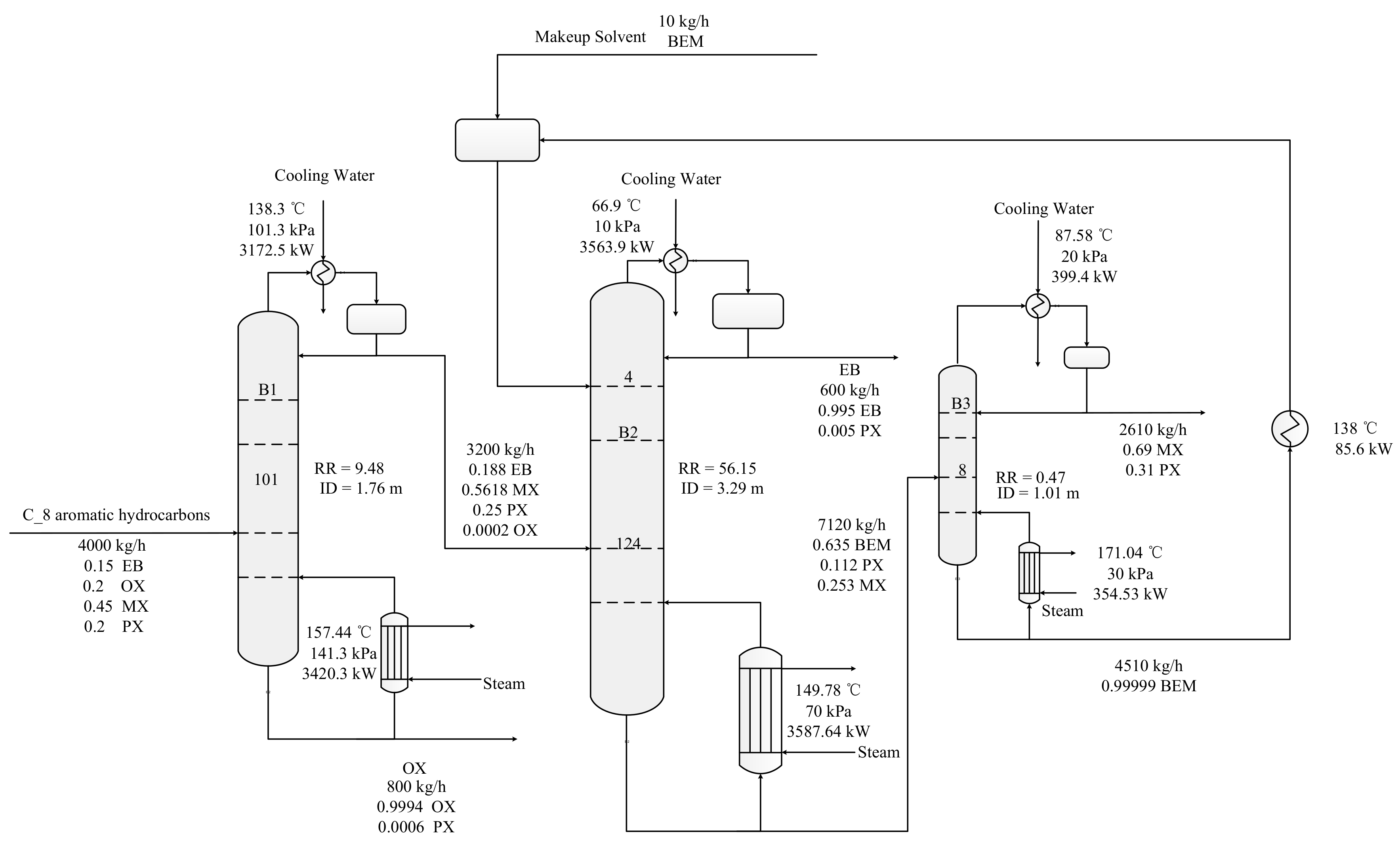
2.1. Steady-State Process

The feed flow was 4000 kg/h with mass concentrations of 0.15, 0.2, 0.45, and 0.2 for ethylene, o-xylene, m-xylene, and p-xylene, respectively. The feed temperature was 30 °C, and the pressure was 200 kPa. Column B1 was used to separate o-xylene from the bottom of the column. The purity of o-xylene was 0.999 (wt.). Column B2 was an extractive distillation, which was used to separate ethylbenzene from the top of the column. The purity of ethylbenzene was 0.995 (wt.). Column B3 was an extractant recovery column, which was used to separate methyl phenylacetate from the bottom of the column. The purity of methyl phenylacetate was 0.999 (wt.) [15,16].

2.2. Optimization Methods

2.2.1. Process Evaluation Indexes

As a common indicator to evaluate the cost of a process, the TAC includes the cost of equipment and utilities. The calculation formula of TAC is as Formula (1) [17]:

TAC = CC/Pay pack Period + OC

(1)

where CC is the capital cost, which includes the cost of column shells, column trays, reboiler, condenser, and vessels. OC is the cost of steam and cooling water. The operation time was 8000 h/year, and the payback period was 3 years. The cost of the distillation column was estimated using Guthrie’s equation [18,19,20,21], as shown in

Table 1. The formulas and parameters of TAC.

Category	Formula	Unit
Column diameter	Aspen tray sizing	m
Column height	H = 0.125 × (N − 2)	m
Column shell cost	shell = 141,320 × D1.066 × H0.802	$
Column stage cost	packing = 12,000 × 3.14/4 × D2 × H	$
Exchanger area	Area = Q/K/ΔTln	m2
Heat exchanger cost	Exchanger = 6.2 × (8500 + 409 × Area0.85)	$
Capital investment	CC = (shell + packing + Exchanger) × 2	$
Heat transfer coefficient	KCB1 = 1864.6	kW/(K × m2)
	KCB2 = 304.7
	KCB3 = 789.2
	KRB1 = 605.58
	KRB2 = 862.74
	KRB3 = 613.53
Utilities cost	Cooling water: 0.03	$
	HP steam (527 K, 1.5 MPa): 25	$

.

The indicator of environmental performance was CO₂ emissions. The CO₂ emissions in the distillation process mainly came from the reboiler at the bottom of the column, which was calculated using Formula (2).

[CO₂]_emission= Q _Fuel × Fuel _Fact.

(2)

where Q _Fuel represents the total heat of fuel combustion in the heating device, kW. This was calculated by Formula (3). Fuel Fact is the amount of carbon dioxide emitted per unit of energy [22], as defined by Formula (4).

$$\mathrm{Q}{ }_{\mathrm{Fuel}}=\frac{{\mathrm{Q}}_{\mathrm{proc}}}{{\mathsf{\lambda }}_{\mathrm{proc}}}({\mathrm{h}}_{\mathrm{proc}}-419)\frac{\mathrm{TFTB}-{\mathrm{T}}_0}{\mathrm{TFTB}-{\mathrm{T}}_{\mathrm{stack}}}$$

(3)

where λ_Proc and hproc represent the latent heat and enthalpy of steam gasification, respectively, kJ/kg. Q_Proc represents the heat duty of the rectifying column, kW. TFTB is the flame temperature of the boiler and Tstack is the chimney temperature, K. T₀ is the ambient temperature, K. The flame temperature was 2073.15 K, the chimney temperature was 433.15 K, and the ambient temjperature was 298.15 K.

$$\mathrm{Fuel}{ }_{\mathrm{Fact}}=(\frac{\mathsf{\alpha }}{\mathrm{NHV}})(\frac{\mathrm{C}\%}{100})$$

(4)

where α represents the ratio of the molar molecular mass of CO₂, and its value was 3.67. NHV is the net calorific value generated by the fuel with C% carbon content. The NHV and C% values of the process were 39,771 kJ/kg and 86.5%, respectively.

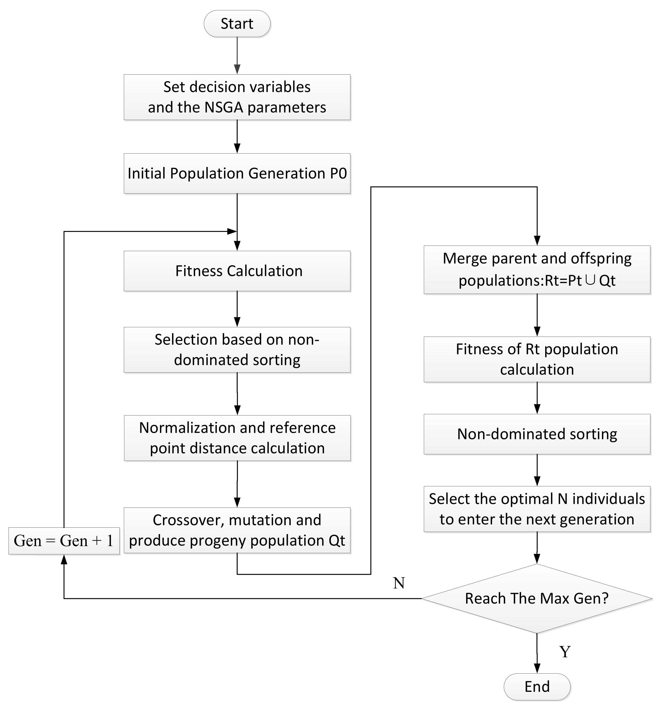
2.2.2. Process Optimization Method

Optimization algorithms are usually divided into two categories. One is a heuristic algorithm that performs optimization calculations based on the information of the problem itself, and the other is a meta-heuristic algorithm that does not use the information of the problem, but searches through algorithm rules. Since the process information could not be obtained in the optimization process of the chemical process, a meta-heuristic algorithm was selected [23]. NSGA-III is a meta-heuristic that does not require explicit information about the mathematical model and its derivatives. The algorithm was suitable for the multi-objective optimization of the chemical process.

A sequential optimization method was used to determine the initial values of the process parameters before the multi-objective optimization. The applied optimization procedure is presented in Figure 1. A random number generator was used to generate the initial population in the search space, and the labeled generation was 0. The initial population was passed into Aspen Plus to obtain the process condition data for the calculation of the fitness function value, and the population was ranked non-dominated according to the calculated fitness function value. A part of the individuals was selected from the sorted population set to perform crossover mutation according to a certain probability. Then, the offspring population was obtained. At this time, the number of generations was added to 1. If the number of iterations reached the set value, the search ended. If not, it was merged with the parent and searched again as a new population [24]. When the search ended, the Pareto front was computed. The ideal point distance method was used as the final solution to calculate the distance between each point in the Pareto front and the ideal point. The point with the smallest distance was selected as the final solution.

The TAC and CO₂ emissions were chosen as the two indicators for the non-dominated ranking. Herein, the TAC and CO₂ emissions were minimized by GA optimization [25,26], which could be simplified in Formula (5).

$$\mathrm{Objective} \mathrm{function} \left\{\begin{array}{c}min TAC\\ min ECO2 \end{array}\right.$$

(5)

Subject to:

X _O-XYL-01 ≥ 0.999

X _EB ≥ 0.995

X _BEM ≥ 0.999

where ECO₂ is the CO₂ emissions, X_O-XYL-01 is the mass purity of o-xylene, the mass purity of ethyl benzene is denoted as X_EB, and X_BEM represents the mass purity of methyl phenylacetate. The decision variables were the number of trays and the feed stage of the three columns.

The search results could be affected by mutation probability and crossover probability. It was necessary to adjust the mutation probability and crossover probability to improve the algorithm’s search performance. In this paper, the performance of the algorithm was evaluated by HV (supervolume index (Formula (6))) and spacing (standard deviation of spatial point distance (Formula (7))).

$$\mathrm{HV}(\mathrm{P})={{\displaystyle \bigcup }}_{\mathrm{x}\in \mathrm{P}}\mathrm{vol}\left(\mathrm{x}\right)$$

(6)

where P is the Pareto front, x is the point in the Pareto front, and vol(x) represents the topological measure value formed by x points in a real Pareto before clicking on P.

$$\mathrm{Spacing}=\sqrt{\frac{1}{|\mathrm{P}|-1}{{\displaystyle \sum }}_{\mathrm{I}=1}^{|\mathrm{P}|}{\left(\mathrm{di}-\overline{\mathrm{d}}\right)}^2}$$

(7)

where |P| represents the number of points in the Pareto front, di is the distance from point i to the other points, and $\overline{\mathrm{d}}$ is the average of all distances.

2.3. Dynamic Simulation Method

During the process, the disturbance of actual operation variables would cause the fluctuation of product concentration. From the steady state to dynamic calculation, it was necessary to calculate the size of the equipment. The tray spacing was 0.125 m. The liquid residence time was 5 min as the benchmark and a 50% margin was left. The height–diameter ratio of the tank was set to 2:1, and the diameter of the tank was calculated with the following Formula (8).

$$\mathrm{V}= \frac{\mathsf{\pi }}{4}{\mathrm{D}}^2\times \left(2\mathrm{D}\right)$$

(8)

where V is the volume of the tank and D is the diameter of the tank.

The temperature-sensitive tray of the rectifying column was calculated with the open-loop gain method. Introducing a 0.1% reboiler heat load fluctuation while keeping other operation variables constant, a new tray temperature profile could be obtained. Using the difference of the temperature distribution of the tray before and after the reboiler heat load disturbance, the steady-state gain value K was obtained through dividing the temperature distribution difference by the reboiler heat load disturbance value, which could be defined as Formula (9).

K = ΔT_S/ΔR

(9)

where K is the steady state gain value, ΔT_S represents the temperature difference of the tray, and ΔR is the heat duty difference of reboiler.

The integral absolute error (IAE) value and response time were used as the evaluation indexes of the control performance of the distillation column. The control performance was better when the IAE value was smaller and the response time was shorter. The IAE was defined as Formula (10).

$$\mathrm{IAE}={{\displaystyle \int }}_0^T\left|\mathrm{e}\left(\mathrm{t}\right)\right|\mathrm{dt}$$

(10)

where e represents the deviation between the measured value and the set value and T is dynamic simulation time.

3. Results and Discussion

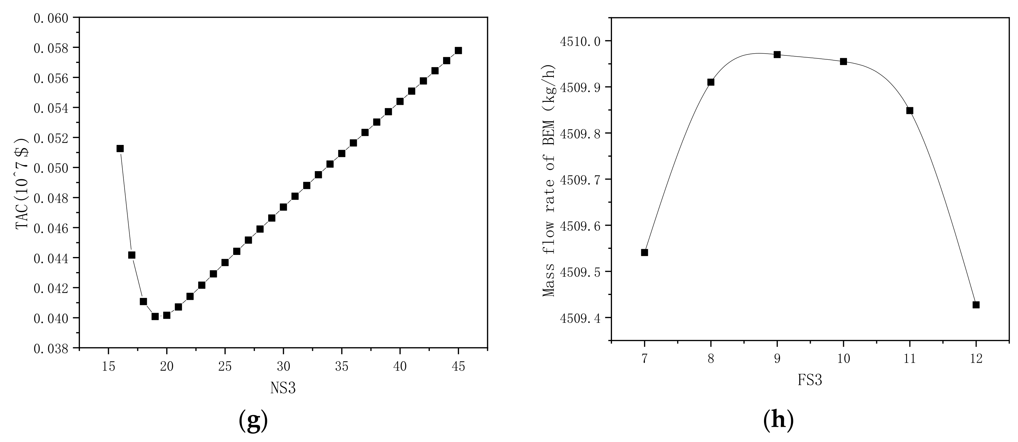
3.1. Sequence Optimization

The sequence optimization method was used to determine the initial process parameters of the process. The main parameters of the process included the number of stages of B1 (NS1), the feed location of B1 (FS1), the number of stages of B2 (NS2), the flowrate of the extraction agent (EF), the feed location of extracting agent (ES), the number of stages of B3 (NS3), and the feed location of B3 (FS3). The total stage number of the column was determined by the minimum TAC. The extractant dosage was determined by the purity of ethylbenzene. The optimum feed location was determined by the maximum product mass flow rate.

The constraint condition of column B1 was that the quality purity of o-xylene at the bottom of the column was greater than 0.999. As shown in Figure 2, the optimum process conditions for column B1 were NS1 = 146 and FS1 = 83. Under optimum conditions, the TAC was the smallest, the mass flow rate of o-xylene was the largest, and the reflux ratio was 15.83.

In column B2, the constraint condition was that the purity of ethylbenzene at the top of the column was greater than 0.995. Figure 3c,d shows that the optimal tray number was 248, and the optimal feed location was at the 128th tray. As shown in Figure 3e, when the extractant flow rate was 4025 kg/h, and the mass purity of ethylbenzene just reached 0.995. In order to ensure the mass purity of ethylbenzene, the extraction agent flow rate was selected as 4500 kg/h. As shown in Figure 3f, the optimal feed location of extractant was at the fourth tray.

Column B3 was the extractant recovery column, and the constraint condition was that the mass purity of methyl benzoate at the bottom of the column was greater than 0.999. Figure 3g,h shows that the TAC value was the smallest when the number of trays in column B3 was nineteen, and the best feed location was at the ninth tray.

Table 2. The result of sequence optimization.

	B1	B2	B3	Total
NS	146	248	19	\
FS	83	4/128	9	\
Reflux ratio	15.83	64.5	0.49	\
TAC (107 $/year)	0.553	1.015	0.040	1.608
[CO2]emissions (ton/year)	10,056.96	7082.08	676.56	17,815.60

shows the detailed comparisons of all the processes. The lowest TACs of the three columns were 0.553 × 10⁷ USD/year, 1.015 × 10⁷ USD/year, and 0.04 × 10⁷ USD/year, respectively. Column B2 had the largest TAC and column B1 had the largest CO₂ emissions.

In this section, sequence optimization method was used to obtain the initial process parameters of the extractive distillation process. The results showed that column B2 had the highest cost among the three columns, and column B1 had the largest CO₂ emissions.

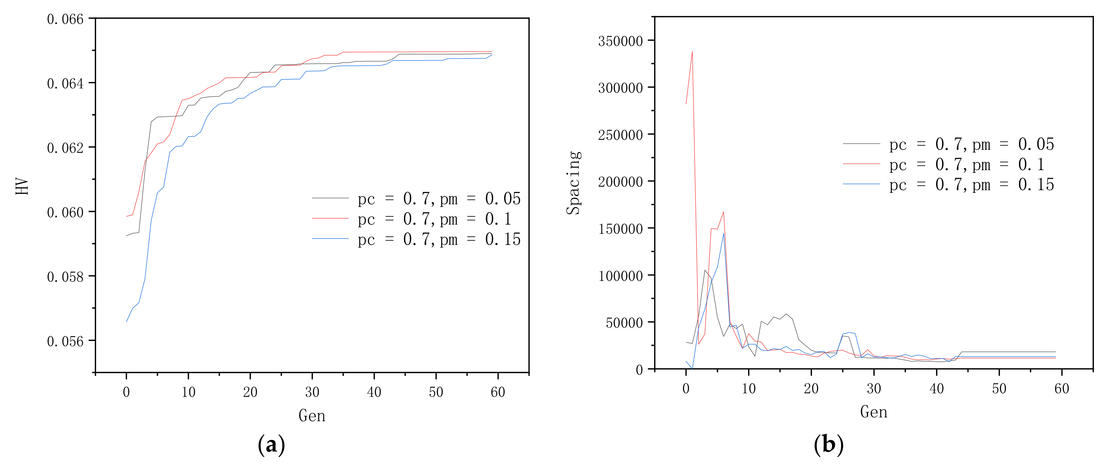
3.2. Optimization of Genetic Algorithm Parameter

In the optimization process of the genetic algorithm, the setting of the mutation probability and crossover probability affected the final result of the algorithm.

The crossover probability pc was fixed at 0.7, and the mutation probability pm was set as 0.05, 0.1, and 0.15. The influence of the mutation probability pm on HV and spacing was discussed. The results are shown in Figure 4. When the mutation probability pm was 0.1, HV converged the fastest and reached the true Pareto frontier at the 30th generation. The standard deviation of the distance between the spatial points near the Pareto frontier was the smallest. Therefore, the mutation probability was selected as 0.1.

The mutation probability pm was fixed at 0.1, and the crossover probability pc was set as 0.7, 0.8, and 0.9. The influence of the crossover probability pc on HV and spacing was studied. The results are shown in Figure 5. When the crossover probability was 0.8, HV converged the fastest in the 24th generation, reaching the true Pareto frontier. The standard deviation of the distance between the spatial points near the Pareto frontier was the smallest. Therefore, the crossover probability was determined to be 0.8.

The influences of the mutation probability and crossover probability on the optimization results under different iterations are shown in Figure 6. It could be seen from Figure 6a–c that when the crossover probability was 0.8, the algorithm converged the fastest and converged to the 24th generation Pareto frontier. When the crossover probability was 0.7 and 0.9, both converged in the 36th generation. As shown in Figure 6a,d,e, when the mutation probability was 0.1, the search performance was the best. When the mutation probability was 0.05, the number of pre-Pareto solutions was the least. When the mutation probability was 0.15, the convergence was the slowest.

Finally, the Pareto frontier with a mutation probability of 0.1 and a crossover probability of 0.8 was selected as the final solution set, which had a total of 36 non-inferior solutions.

This subsection investigated the influence of different settings of the parameters of NSGA-III on the searching process. The results showed that the best mutation probability was 0.1, the best crossover probability was 0.8, and the suitable numbers of generations of the algorithm was 60.

3.3. The Global Optimal Solution

Figure 7 shows the Pareto optimal boundaries of the TAC and ECO₂ after 60 iterations. The solution set consisted of 36 solutions, each of which was a Pareto optimal solution. In Figure 7a, Opt point 1 was the minimum point of the TAC, and was the maximum point of CO₂ emissions. Conversely, Opt point 2 was the maximum point of the TAC, and was the minimum point of CO₂ emissions. Therefore, it was necessary to choose a point among them as the optimal solution. The ideal point distance method is a common method used to calculate the global optimal value. A straight line was made perpendicular to the horizontal axis through Opt point1, and a straight line was made perpendicular to the vertical axis through Opt point 2. The intersection of two lines was the ideal point of the solution set. The distance from each point in the solution set to the ideal point was calculated, and the results are shown in Figure 7b. It could be seen from Figure 7b that the 32nd scheme was the optimal scheme. The TAC value of this scheme was 1.420 × 107 USD/year, and the CO₂ emissions value was 13,588.6 kg/h.

As shown in

Table 3. The result of multiple-objective optimization.

	B1	B2	B3	Total
NS	180	252	15	\
FS	101	4/128	6	\
Reflux ratio	9.48	56.15	0.47	\
TAC (107 $/year)	0.432	0.950	0.038	1.420
[CO2]emissions (kg/h)	6294.4	6646.4	647.8	13,588.6

, under the optimization of the NSGA algorithm, the total TAC and CO₂ emissions both decreased. The number of trays in column B1 increased from 146 to 180, and the reflux ratio decreased from 15.83 to 9.48. The number of trays in column B2 increased from 248 to 252, and the reflux ratio decreased from 64.5 to 56.15. The number of trays in column B3 was reduced from 19 to 15, and the reflux ratio was reduced from 0.49 to 0.47. The total TAC dropped by 11.7%, and total CO₂ emissions dropped by 23.7%.

Based on the final Pareto front, this subsection used the ideal point distance method to find the global optimal solution. The results showed that the TAC of the final solution decreased by 11.7% and the CO₂ emissions of the final solution decreased by 23.7% compared with the initial value.

4. Dynamic Control

According to the optimization results in Table 2, the process flow shown in Figure 8 was obtained. When a steady state model was switched to a dynamic model, the dimensions of the device were be calculated first. The diameter and height of the reflux tanks of column B1 were 1.8 m and 3.6 m, respectively. Similarly, the diameters of the reflux tanks of column B2 and B3 were 1.7 m and 1.0 m respectively, and the height of reflux tanks of column B2 and B3 were 3.4 m and 2.0 m, respectively.

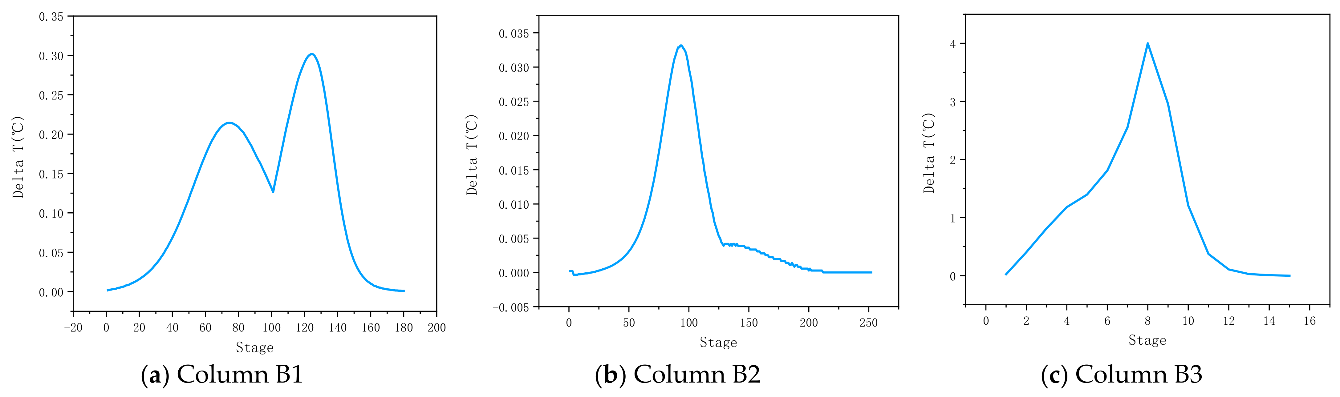
4.1. Determination of Temperature-Sensitive Tray

During the dynamic operation of the distillation column, the disturbance would lead to a rapid temperature change in some trays, which would affect the purity of products. Therefore, the temperature-sensitive tray should be determined before designing control structure. Herein, the position of the temperature-sensitive tray was determined by the open-loop gain method. When the heat duty of the reboiler increased by 0.1%, the temperature distribution before and after the increase was different and divided by the open-loop gain of the reboiler heat load disturbance for the column temperature, as shown in Figure 9. According to Figure 9a, column B1 had two sensitive trays, which were the 74th stage and the 124th stage. According to Figure 9b, the 85th sensitive tray was the sensitive tray of column B2. Similarly, Figure 9c shows that the sensitive tray of column B3 was the 8th tray.

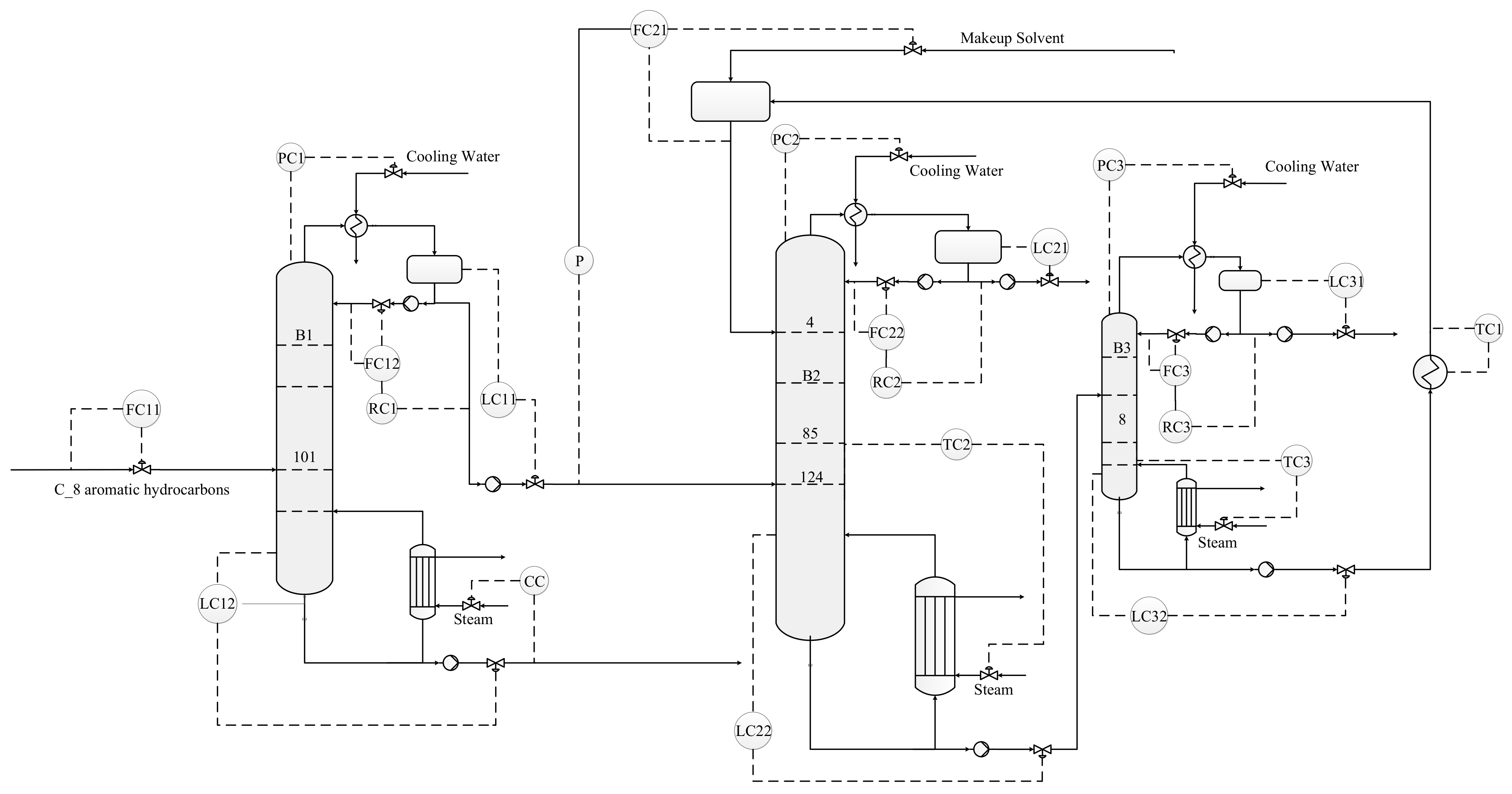
4.2. Basic Control Structure for Circulating Flow Rate of Extractant (CS1)

First of all, a conventional extractant circulation flow control structure is shown in Figure 10. To stabilize the purity of the product, some control strategies were added in CS1. The overall basic control loops are illustrated as below [27,28,29]:

• The feed flow rate was controlled by a throughput valve (reverse action).
• The liquid level of the reflux tank was manipulated by the distilled flow rates (positive action).
• The sump level of the column of B1 and B2 was manipulated by the bottom flowrate (positive action).
• The sump level of the column of B3 was controlled by the flow of entrainer makeup (reverse action).
• All pressure in the three columns were controlled by manipulating the top condenser duties.
• The reflux ratios in the three columns were fixed.
• The temperature of the recycling solvent was controlled by a heat exchanger (reverse action).
• The recycled solvent flowrate was rationed to the distilled flow rates of column B1 and controlled by a throughput valve (reverse action).
• The temperature of the sensitive tray of the column of B1 was controlled by component controller to manipulate the reboiler duty of column B1 (reverse action).
• The temperatures of the sensitive trays of the columns of B2 and B3 were controlled by changing the reboiler heat duty (reverse action).

Figure 10. Control structure 1 (CS1).

Figure 10. Control structure 1 (CS1).

All controllers were PI controllers. The parameters of the liquid level controller were set as Kc = 2 and τ_I = 9999 min. The top pressure control loop parameters of the three columns were set as Kc =20 and τ_I =12 min. The feed flow controller was set as Kc = 0.5 and τI = 0.3 min. The missing parameters of the temperature and component controller were obtained by the Tyreus–Luyben tuning method.

Table 4. Controller gain and integration time.

	CS1		CS2
	Gain	Integral Time (min)	Gain	Integral Time (min)
CC	5675	28	5297	30.1
TC1	3.1	13.2	3.7	13.2
TC2	8.9	76.7	8.9	76
TC3	2.1	18.5	1.1	23.8

shows the controller tuning parameters:

Flow and composition disturbances were added to examine the dynamic response to the process. After adding the concentration controller, the o-xylene product of column B1 stabilized at 0.99935, so it will not be discussed further. The dynamic responses of CS1 at a ±10% feed flow rate disturbance are shown in Figure 11. The first sensitive plate of B1 was stabilized in 5 h with a temperature fluctuation of 1.7 °C, and the second sensitive plate was equilibrated in 4 h with a temperature fluctuation of 3.2 °C. The temperature of the sensitive tray of B2 was stabilized within 17 h, and the fluctuation range of the temperature was 0.1 °C. The temperature of the sensitive tray of B3 was stable within 10 h, and the fluctuation range of the temperature was 15 °C. The EB concentration of B2 was stable within 13 h, and the fluctuation range of the concentration was 0.001. The BEM concentration of B3 was stable within 10 h, and the fluctuation range of the concentration was 0.0004.

The dynamic responses of the CS1 structure to the concentration disturbance are shown in Figure 12. The first sensitive plate of B1 reached a stable state within 20 h with a temperature fluctuation of 0.548 °C, and the second sensitive plate reached a stable state within 16 h with a temperature fluctuation of 0.031 °C. The sensitive plate of B2 was stable within 16 h with a temperature fluctuation of 0.007 °C, and the sensitive plate of B3 was stable within 8 h with a temperature fluctuation of 0.000002 °C. The EB concentration of B2 was stable within 20 h, and the fluctuation range of the concentration was 0.0001. The BEM concentration of B3 was stable within 8 h, and the fluctuation range of the concentration was 0.0000002.

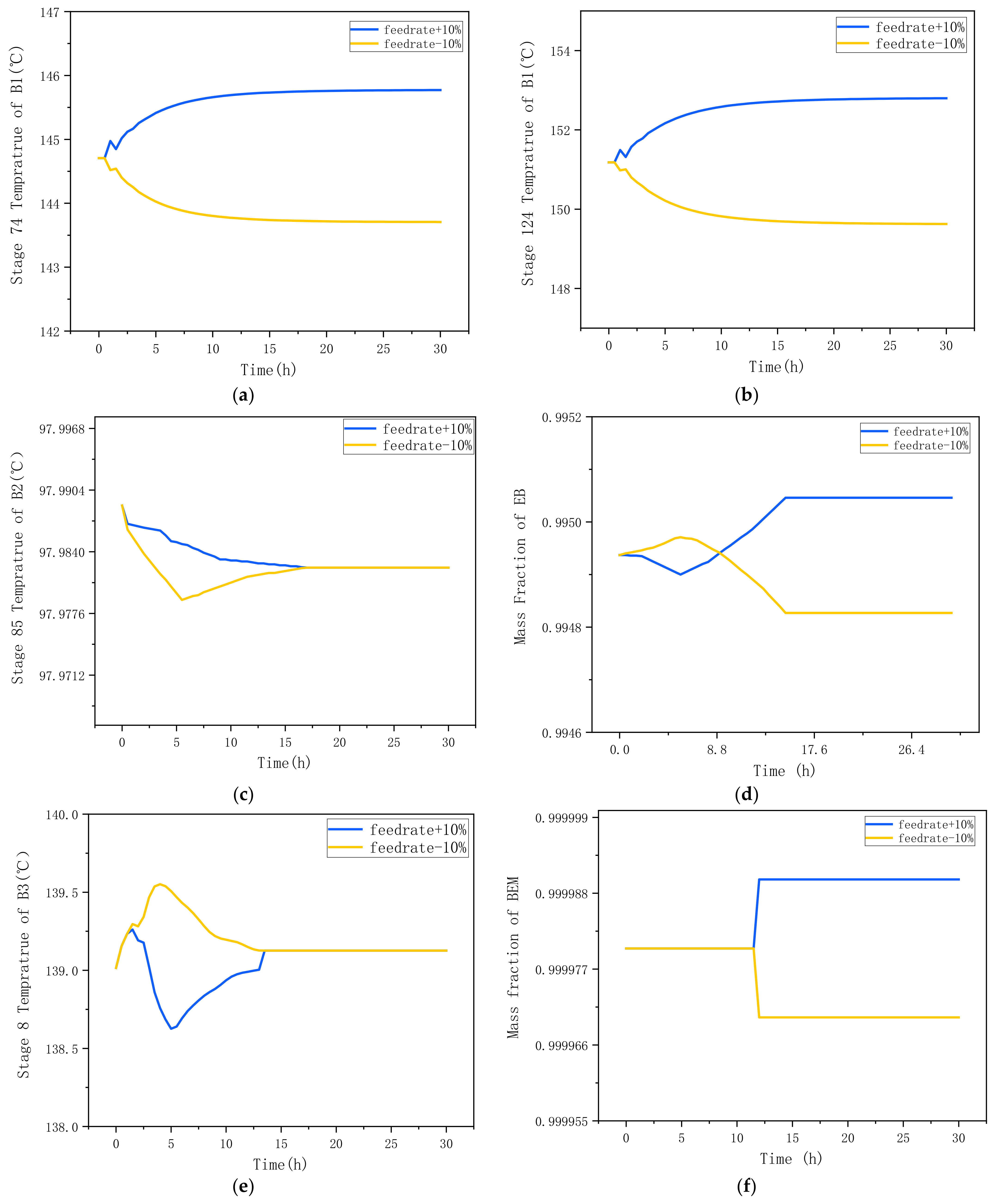
4.3. An Improved Control Structure (CS2)

In order to stabilize the sensitive tray temperature of column B3, the control structure of CS1 was improved. The liquid level of the column bottom was controlled by controlling the flow of the column bottom, and the circulation flow of extractant was maintained by controlling the make-up amount of extractant. The reflux flow of column B1 was determined by the feed flow. The improved structure is shown in Figure 13.

A ±10% feed flow rate disturbance was added to the CS2 control structure. The results are shown in Figure 14. The temperature of the first sensitive plate of column B1 was stable within 15 h with a temperature fluctuation of 1.8 °C, and the second sensitive plate was balanced within 15 h with a temperature fluctuation of 3 °C. The temperature of the sensitive plate of column B2 was stable within 15 h with a temperature fluctuation amplitude of 0.014 °C. The EB concentration of B2 was stable within 21 h, and the fluctuation range of the concentration was 0.0001. The temperature of column B3 was stable within 14 h with a temperature fluctuation amplitude of 1 °C. The BEM concentration of B3 was stable within 12 h, and the fluctuation range of the concentration was 0.00002. Compared with CS1, the temperature fluctuation of the sensitive plate of column B3 under the control of CS2 was significantly reduced.

The dynamic responses of the CS2 structure to the concentration disturbance are shown in Figure 15. The first sensitive tray was stable within 12 h with a temperature fluctuation of 0.554 °C, and the second sensitive tray was stable within 25 h with a temperature fluctuation of 0.055 °C. The sensitive plate of B2 was stable within 15 h with a temperature fluctuation of 0.014 °C, and the sensitive plate of B3 was stable within 17 h with a temperature fluctuation of 0.15 °C. The EB concentration of B2 was stable within 21 h, and the fluctuation range of the concentration was 0.0001. The BEM concentration of B3 was stable within 8 h, and the fluctuation range of the concentration was 0.000004. Under the concentration disturbance, the performance of the two control strategies was similar.

In this section, two control strategies were designed, namely, the flowrate of the entraining agent (CS1) and the flowrate of the extractant recovery column (CS2) to control the flowrate of solvent recovery. The results showed that two control strategies had similar performances in resisting the concentration disturbance, but CS2 had a better performance against flow disturbance. To sum up, the CS2 control strategy should be selected for this process.

5. Conclusions

An extractive distillation process was proposed for the separation of ethylbenzene from a C₈ aromatic hydrocarbon mixture species. The TAC and CO₂ emissions of the process were optimized by NSGA-III. A new control strategy for the extractive distillation process was designed.

A distillation process for the separation of ethylbenzene was designed using methyl phenylacetate as an extractant. The economic and environmental effects of the process were studied with a sequence optimization method and a genetic algorithm. The sequential optimization method was used to obtain the initial process parameters. Then, the total annual cost and CO₂ emissions were minimized by NSGA-III. When the mutation probability was 0.1 and the crossover probability was 0.8, the genetic algorithm had the largest hypervolume index value and the smallest spatial point distance variance. The optimal total annual cost and CO₂ emissions were 11.7% and 23.7% lower than those of the initial process. Based on the steady process, Aspen Dynamic was used to assess the dynamic performance. Two control strategies, which were the flow rate of the recycling solvent controlled by entrainer makeup flowrate (CS1) and the bottom flow rate of the extractant recovery column (CS2), were established. The calculation results showed that the CS2 structure was more stable in terms of process parameters than CS1, especially in terms of the temperature control of the extractant recovery column.

The future work of this paper will focus on the extension of the existing processes and in-depth research on more advanced control strategies, and we will apply the results of this research to industrialization.

References

1. Pandit, S.R.; Jana, A.K. Transforming conventional distillation sequence to dividing wall column: Minimizing cost, energy usage and environmental impact through genetic algorithm. Sep. Purif. Technol. 2022, 297, 121437. [Google Scholar] [CrossRef]
2. You, X.; Gu, J.; Gerbaud, V.; Peng, C.; Liu, H. Optimization of pre-concentration, entrainer recycle and pressure selection for the extractive distillation of acetonitrile-water with ethylene glycol. Chem. Eng. Sci. 2018, 177, 354–368. [Google Scholar] [CrossRef] [Green Version]
3. Gu, J.; You, X.; Tao, C.; Li, J. Analysis of heat integration, intermediate reboiler and vapor recompression for the extractive distillation of ternary mixture with two binary azeotropes. Chem. Eng. Process. Process Intensif. 2019, 142, 107546. [Google Scholar] [CrossRef]
4. Han, D.; Chen, Y.; Shi, D. Different extractive distillation processes for isopropanol dehydration using low transition temperature mixtures as entrainers. Chem. Eng. Process. Process Intensif. 2022, 178, 109049. [Google Scholar] [CrossRef]
5. Yang, A.; Yang Kong, Z.; Sunarso, J.; Su, Y.; Wang, Q.; Zhu, S. Insights on sustainable separation of ternary azeotropic mixture tetrahydrofuran/ethyl acetate/water using hybrid vapor recompression assisted side-stream extractive distillation. Sep. Purif. Technol. 2022, 290, 120884. [Google Scholar] [CrossRef]
6. Shi, T.; Chun, W.; Yang, A.; Su, Y.; Jin, S.; Ren, J.; Shen, W. Optimization and control of energy saving side-stream extractive distillation with heat integration for separating ethyl acetate-ethanol azeotrope. Chem. Eng. Sci. 2020, 215, 115373. [Google Scholar] [CrossRef]
7. Hou, Y.; Wu, N.; Li, Z.; Zhang, Y.; Qu, T.; Zhu, Q. Many-objective optimization for scheduling of crude oil operations based on NSGA-III with consideration of energy efficiency. Swarm Evol. Comput. 2020, 57, 100714. [Google Scholar] [CrossRef]
8. Jaime, J.A.; Rodríguez, G.; Gil, I.D. Control of an Optimal Extractive Distillation Process with Mixed-Solvents as Separating Agent. Ind. Eng. Chem. Res. 2018, 57, 9615–9626. [Google Scholar] [CrossRef]
9. Qin, J.; Ye, Q.; Xiong, X.; Li, N. Control of Benzene–Cyclohexane Separation System via Extractive Distillation Using Sulfolane as Entrainer. Ind. Eng. Chem. Res. 2013, 52, 10754–10766. [Google Scholar] [CrossRef]
10. Ahmadian Behrooz, H. Robust Design and Control of Extractive Distillation Processes under Feed Disturbances. Ind. Eng. Chem. Res. 2017, 56, 4446–4462. [Google Scholar] [CrossRef]
11. Yu, B.; Wang, Q.; Xu, C. Design and Control of Distillation System for Methylal/Methanol Separation. Part 2: Pressure Swing Distillation with Full Heat Integration. Ind. Eng. Chem. Res. 2012, 51, 1293–1310. [Google Scholar] [CrossRef]
12. Lu, J.; Wang, Q.; Zhang, Z.; Tang, J.; Cui, M.; Chen, X.; Liu, Q.; Fei, Z.; Qiao, X. Surrogate modeling-based multi-objective optimization for the integrated distillation processes. Chem. Eng. Process. Process Intensif. 2021, 159, 108224. [Google Scholar] [CrossRef]
13. Yamanee-Nolin, M.; Andersson, N.; Nilsson, B.; Max-Hansen, M.; Pajalic, O. Trajectory optimization of an oscillating industrial two-stage evaporator utilizing a Python-Aspen Plus Dynamics toolchain. Chem. Eng. Res. Des. 2020, 155, 12–17. [Google Scholar] [CrossRef]
14. Zhang, H.; Zhao, Q.; Zhou, M.; Cui, P.; Wang, Y.; Zheng, S.; Zhu, Z.; Gao, J. Economic effect of an efficient and environmentally friendly extractive distillation/pervaporation process on the separation of ternary azeotropes with different compositions. J. Clean. Prod. 2022, 346, 131179. [Google Scholar] [CrossRef]
15. Gil, I.D.; Botía, D.C.; Ortiz, P.; Sánchez, O.F. Extractive Distillation of Acetone/Methanol Mixture Using Water as Entrainer. Ind. Eng. Chem. Res. 2009, 48, 4858–4865. [Google Scholar] [CrossRef]
16. Chen, J.; Ye, Q.; Liu, T.; Xia, H.; Feng, S. Improving the performance of heterogeneous azeotropic distillation via self-heat recuperation technology. Chem. Eng. Res. Des. 2019, 141, 516–528. [Google Scholar] [CrossRef]
17. Ahmed, M.; Abdullah, A.; Laskar, A.; Patle, D.S.; Vo, D.N.; Ahmad, Z. Process simulation and stochastic multiobjective optimisation of homogeneously acid-catalysed microalgal in-situ biodiesel production considering economic and environmental criteria. Fuel 2022, 327, 125165. [Google Scholar] [CrossRef]
18. Gutiérrez-Guerra, R.; Segovia-Hernández, J.G.; Hernández, S. Reducing energy consumption and CO2 emissions in extractive distillation. Chem. Eng. Res. Des. 2009, 87, 145–152. [Google Scholar] [CrossRef]
19. Di Pretoro, A.; Montastruc, L.; Manenti, F.; Joulia, X. Flexibility assessment of a biorefinery distillation train: Optimal design under uncertain conditions. Comput. Chem. Eng. 2020, 138, 106831. [Google Scholar] [CrossRef]
20. Gadalla, M.A.; Olujic, Z.; Jansens, P.J.; Jobson, M.; Smith, R. Reducing CO2 Emissions and Energy Consumption of Heat-Integrated Distillation Systems. Environ. Sci. Technol. 2005, 39, 6860–6870. [Google Scholar] [CrossRef]
21. Gu, J.; You, X.; Tao, C.; Li, J.; Gerbaud, V. Energy-Saving Reduced-Pressure Extractive Distillation with Heat Integration for Separating the Biazeotropic Ternary Mixture Tetrahydrofuran–Methanol–Water. Ind. Eng. Chem. Res. 2018, 57, 13498–13510. [Google Scholar] [CrossRef] [Green Version]
22. Liu, J.; Ren, J.; Yang, Y.; Liu, X.; Sun, L. Effective semicontinuous distillation design for separating normal alkanes via multi-objective optimization and control. Chem. Eng. Res. Des. 2021, 168, 340–356. [Google Scholar] [CrossRef]
23. Liu, Q.; Liu, X.; Wu, J.; Li, Y. An Improved NSGA-III Algorithm Using Genetic K-Means Clustering Algorithm. IEEE Access 2019, 7, 185239–185249. [Google Scholar] [CrossRef]
24. Suggala, S.V.; Bhattacharya, P.K. Real Coded Genetic Algorithm for Optimization of Pervaporation Process Parameters for Removal of Volatile Organics from Water. Ind. Eng. Chem. Res. 2003, 42, 3118–3128. [Google Scholar] [CrossRef]
25. Sohani, A.; Delfani, F.; Hosseini, M.; Sayyaadi, H.; Karimi, N.; Li, L.K.B.; Doranehgard, M.H. Dynamic multi-objective optimization applied to a solar-geothermal multi-generation system for hydrogen production, desalination, and energy storage. Int. J. Hydrogen Energy 2022, 47, 31730–31741. [Google Scholar] [CrossRef]
26. Li, W.; Shi, L.; Yu, B.; Xia, M.; Luo, J.; Shi, H.; Xu, C. New Pressure-Swing Distillation for Separating Pressure-Insensitive Maximum Boiling Azeotrope via Introducing a Heavy Entrainer: Design and Control. Ind. Eng. Chem. Res. 2013, 52, 7836–7853. [Google Scholar] [CrossRef]
27. Kong, Z.Y.; Yang, A.; Segovia Hernández, J.G.; Putranto, A.; Sunarso, J. Towards sustainable separation and recovery of dichloromethane and methanol azeotropic mixture through process design, control, and intensification. J. Chem. Technol. Biotechnol. 2022. [Google Scholar] [CrossRef]
28. Li, D.; Zeng, F.; Jin, Q.; Pan, L. Applications of an IMC based PID Controller tuning strategy in atmospheric and vacuum distillation units. Nonlinear Anal. Real World Appl. 2009, 10, 2729–2739. [Google Scholar] [CrossRef]
29. Shen, W.; Chien, I. Design and Control of Ethanol/Benzene Separation by Energy-Saving Extraction–Distillation Process Using Glycerol as an Effective Heavy Solvent. Ind. Eng. Chem. Res. 2019, 58, 14295–14311. [Google Scholar] [CrossRef]
Figure 1. Process diagram of C8 aromatics extractive distillation.
Processes 10 02237 g001
Figure 2. Optimization procedures of NSGA for ED process.
Processes 10 02237 g002
Figure 3. Optimization of NS1 (a), FS1 (b), NS2 (c), FS2 (d), EF (e), ES (f), NS3 (g), and FS3 (h).
Processes 10 02237 g003aProcesses 10 02237 g003b
Figure 4. Effect of mutation probability on HV and spacing: (a) HV with different mutation probability, (b) Spacing with different mutation probability.
Processes 10 02237 g004
Figure 5. Effect of crossover probability on HV and spacing: (a) HV with different mutation probability, (b) Spacing with different mutation probability.
Processes 10 02237 g005
Figure 6. Influence of mutation probability and crossover probability on optimization results under different iteration times.
Processes 10 02237 g006
Figure 7. Pareto front of the optimal solution: (a) The calculation diagram of the global optimal solution; (b) the number of the ideal point distance of the solution.
Processes 10 02237 g007
Figure 8. Process flow chart of C8 aromatics extractive distillation.
Processes 10 02237 g008
Figure 9. The open-loop sensitivity plots for +0.1% increase in reboiler duty of three columns.
Processes 10 02237 g009
Figure 11. Dynamic responses for CS1 with ±10% feed flow rate disturbance: (a) the temperature of the first sensitive tray in column B1, (b) the temperature of the second sensitive tray in column B1, (c) the temperature of the sensitive tray in column B2, (d) mass concentration of EB at the top of the column B2, (e) the temperature of the sensitive tray in column B3, (f) mass concentration of BEM at the bottom of the column B3.
Processes 10 02237 g011
Figure 12. Dynamic responses for CS1 with feed composition disturbances: (a) the temperature of the first sensitive tray in column B1, (b) the temperature of the second sensitive tray in column B1, (c) the temperature of the sensitive tray in column B2, (d) mass concentration of EB at the top of the column B2, (e) the temperature of the sensitive tray in column B3, (f) mass concentration of BEM at the bottom of the column B3.
Processes 10 02237 g012
Figure 13. Control structure 2 (CS2).
Processes 10 02237 g013
Figure 14. Dynamic responses for CS2 with ±10% feed flow rate disturbance: (a) the temperature of the first sensitive tray in column B1, (b) the temperature of the second sensitive tray in column B1, (c) the temperature of the sensitive tray in column B2, (d) mass concentration of EB at the top of the column B2, (e) the temperature of the sensitive tray in column B3, (f) mass concentration of BEM at the bottom of the column B3.
Processes 10 02237 g014
Figure 15. Dynamic responses for CS2 with feed composition disturbances: (a) the temperature of the first sensitive tray in column B1, (b) the temperature of the second sensitive tray in column B1, (c) the temperature of the sensitive tray in column B2, (d) mass concentration of EB at the top of the column B2, (e) the temperature of the sensitive tray in column B3, (f) mass concentration of BEM at the bottom of the column B3.
Processes 10 02237 g015