Article

Reinforcement Learning Control with Deep Deterministic Policy Gradient Algorithm for Multivariable pH Process

by
Chanin Panjapornpon
*,
Patcharapol Chinchalongporn
,
Santi Bardeeniz
,
Ratthanita Makkayatorn
and
Witchaya Wongpunnawat
Department of Chemical Engineering, Center of Excellence on Petrochemicals and Materials Technology, Faculty of Engineering, Kasetsart University, Bangkok 10900, Thailand
*
Author to whom correspondence should be addressed.
Processes 2022, 10(12), 2514; https://doi.org/10.3390/pr10122514
Submission received: 7 October 2022 / Revised: 10 November 2022 / Accepted: 21 November 2022 / Published: 26 November 2022

Abstract

:
The pH treatment unit is widely used in various processes, such as wastewater treatment, pharmaceutical manufacturing, and fermentation. It is essential to get the on-specifications product. Thus, controlling pH is key management for accomplishing the manufacturing objective. However, the highly nonlinear pH characteristics of acid–base titration make pH regulation difficult. Applications of artificial intelligence for process control have progressed and gained popularity recently. The development of reinforcement learning (RL) control with a deep deterministic policy gradient (DDPG) algorithm to handle coupled pH and liquid level control in a continuous stirred tank reactor with a strong acid–base reaction is presented in this study. To validate the RL model, the reward functions are created individually for the level and pH controls. The grid search technique is deployed to optimize the hyperparameters of the RL controller models, including the number of nodes in the hidden layers and the number of episodes. The control performance of the proposed RL control system was compared with that of the proportional-integral controller in a servo-regulatory test. The simulation results show that the proposed RL controllers outperform the proportional-integral controllers in approaching setpoints faster, with better performance and less oscillation.

1. Introduction

pH treatment is used extensively in industrial processes to maintain product quality within the desired range of specifications. Therefore, controlling pH is essential for achieving the required product specification. For example, the pH of the effluent stream from a wastewater treatment plant must be maintained within environmental regulations, the pH of the liquid fertilizer must be adjusted to control soil quality and enhance plant growth [1], and the pH of sugarcane juice after bleaching must be treated by alkalinization [2]. Due to the high nonlinearities of pH, advanced control techniques, especially model-based control, have received considerable attention in the design of pH control systems over the past few decades. The model-based controller can be constructed by using both physical and neural models. Chi et al. [3] use the ARX cascaded neural network structure for latent-variable nonlinear model predictive control in pH adjustment. Estofanero et al. [4] used the neural ARIMA model to control the HCl-NaOH neutralization process with a model predictive controller (MPC). Mahmoodi et al. [5] presented a nonlinear predictive control based on the Wiener–Laguerre model to control the pH neutralization process. Although model-based pH control is highly accurate and efficient, it requires more time for process modeling and acid–base reaction determination [6].
The reinforcement learning (RL)-based control has been developed and has evolved for two decades. The RL structure consists of an agent that learns and maps actions to maximize a numerical reward. The deep Q-learning network (DQN) was an early developed RL algorithm that was used to play Atari games by receiving pixels and game scores as inputs. Dressler et al. [7] performed drop microfluidic control using the RL with the DQN algorithm in a real experiment. The deterministic policy gradient (DPG) algorithm was developed by Silver et al. to handle continuous states and actions [8]. Lillicrap et al. presented an actor-critic RL algorithm known as the deep deterministic policy gradient (DDPG) in which the DPG is an actor and the DQN is a critic to control continuous environments. Fujii et al. used the actor-critic RL algorithm to apply a self-tuning two-degree-of-freedom control based on reinforcement learning to film production [9]. The DDPG has some drawbacks requiring numerous training episodes to find the solutions [10]. Yoo et al. applied a Monte Carlo method to improve actor learning in the DDPG algorithm for controlling a batch polymerization process [11].
In this work, an RL-based control system is proposed to handle the coupled pH and liquid level control in a strong acid–base continuous stirred tank reactor. The DDPG is used to develop multiple agents for level control and pH control to make continuous control action decisions for the optimal flow rate of the feed and titrant streams to achieve desired setpoints. In model training, a mathematical model of the pH process is used as the environment, and the reward is calculated based on reward policies that are defined with output errors. The proposed RL controllers are evaluated with the servo-regulatory test under the MATLAB/Simulink environment. The main contributions of this paper can be summarized as follows:
  • Develop the RL control using the multi-DDPG agents to handle the multivariable pH process with highly nonlinear dynamics and use the grid search—hyperparameter tuning technique—to optimize the RL control performance.
  • Study the control performance of the pH and level control by comparing the RL controller with multi-DDPG agents and the multi-single-input and single-output controllers.
The remainder of this work is divided into the following sections: Section 2 integrates the concept of actor-critic learning, which is the base knowledge leading to the DDPG algorithm and presents the grid search hyperparameter tuning concepts with the performance evaluation. Section 3 presents the procedure for RL development for the pH process that consists of process modeling, network, policy design, and algorithm setup. Section 4 shows the performance of the proposed control system with the servo-regulatory test compared with the proportional-integral (PI) control. Finally, conclusions are drawn in Section 5.

2. Preliminary

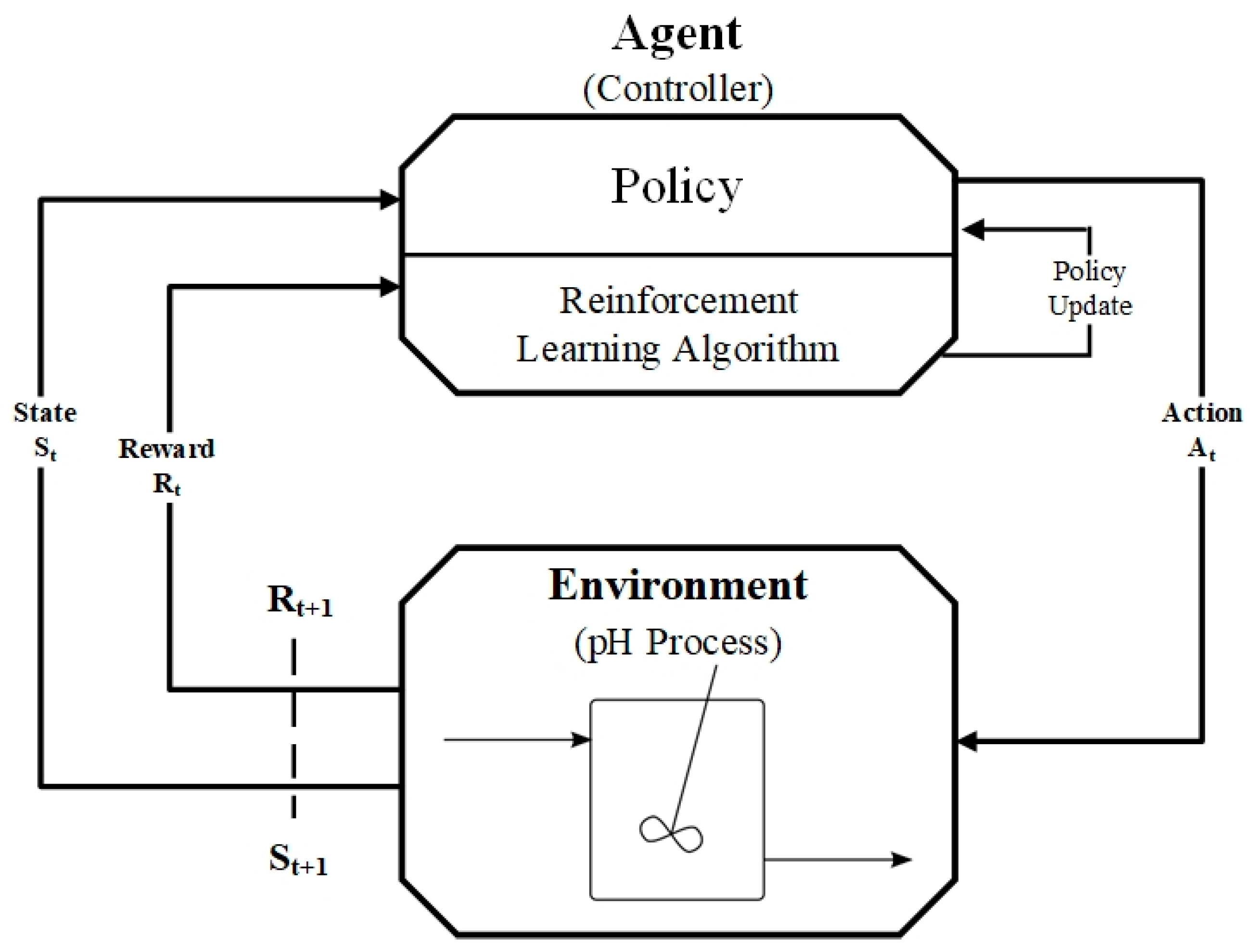
2.1. Reinforcement Learning Control

The process of learning what to do and how to map a situation to action in order to maximize numerical rewards is known as reinforcement learning (RL). RL has been conducting active research in the control system to choose the best control action. Syafiie and colleagues [12] used the model-free learning controller (MFLC) based on reinforcement learning with the Q-learning algorithm for pH process control. In the Q-learning algorithm, Q-values are updated in the Q-table by selecting the optimal action from the maximum Q-value to obtain the optimal policy. Shah and Gopal [13] used a model-free predictive controller based on reinforcement learning to control the coolant flow velocity using a fuzzy inference system (FIS) with Q-learning as an approximator for tuning the PID controller. The disadvantage of Q-learning is that it has a finite set of states and actions. With the improvement in artificial intelligence technology, it has been utilized to improve the RL learning model for making the sequence of decisions. Alves and Dutra [14] proposed the RL pH controller with a particle swarm optimization (PSO) algorithm to vary the RL hyperparameters. The actor-critic algorithm is applied the value function approximation stochastic policy to work with a continuous space of states and actions. Sedighizadeh and Rezazadeh [15] applied the RL-based adaptive PID controller to wind energy conversion systems. Actor-critic learning with a deep neural network (DNN) is used as an approximator for parameters in the PID controller. The actor-critic learning architecture consists of three parts: an actor, a critic, and a stochastic action modifier (SAM). The actor and the critic can use the input data and hidden layers of the DNN together. The SAM is used to generate the actual PID parameters based on the recommended parameters from the actor and the estimated signal from the critic.
As aforementioned, a Q-table approach in which data are filled into the table to select the appropriate value may be unsuitable for a continuous action system learning from large amounts of dynamic data. Furthermore, the application of reinforcement learning in process control has primarily been studied in a single-input and single-output control system. This work has developed a model-based RL controller with multi-DDPG agents with actor-critic neural networks.
Because the pH dynamics are more nonlinear than the liquid level dynamics, implementing a single DDPG agent capable of controlling both the pH and the liquid level at the same time is difficult. In addition, the MATLAB software does not support normalization through an input layer of the actor-critic neural network by default, resulting in diminished learning efficiency. Thus, the DDPG agent has been designed to control the liquid level and pH separately. The RL system has the main characters, which are the agent and the environment. The agent stays and interacts with the environment. The agent observes the state (St) to do an action (At) and gets the reward (Rt) signal returning. Then the environment generates the reward (Rt+1) and the next state (St+1) in each iteration. The agent contains two components which are the policy and the reinforcement learning algorithm. Policy mapping determines an action based on the state of the environment. The learning algorithm updates the policy parameters continuously based on action, state, and reward. The objective of the agent needs to maximize its cumulative reward. The RL overview is shown in Figure 1.
A standard reinforcement is considered when an agent interacts with a stochastic and fully observable environment by choosing the sequent actions in a discrete-time step to calculate the cumulative reward (Gt), which is defined in Equation (1). This series of processes is called the Markov decision process (MDP). It is necessary to reduce the importance of discrete rewards in the future using the discount factor ( γ ), where γ [ 0 , 1 ] is a discount factor that determines the importance of rewards.
G t = R t + 1 + γ R t + 2 + γ 2 R t + 3 + = k = 0 γ k R ( t + 1 ) + k
A state-action value function, Q π ( S t , A t ) , is defined to estimate the performance of an action in the state to maximize the reward following a target policy (𝜋). The long-term reward expectation is earned for each action-value function following Equation (2).
Q π ( S t , A t ) = E π G t S t = S , A t = A
Q-learning is a typical type of off-policy learning that updates a target policy using samples generated by any stochastic behavior policy in an environment. It has the goal of estimating the Q-value or state-action value. Following the Bellman equation for the action-value function, the Q-value is updated by Equation (3). In Q-learning updating, the behavior policy followings an epsilon-greedy exploration strategy to sample the next actions A t + 1 . Then, the A is selected from the action that makes the largest Q-value following the target policy
Q ( S t , A t ) = Q ( S t , A t ) + α r t + 1 + γ max A A Q ( S t + 1 , A ) Q ( S t , A t )
where α is the learning rate.

2.2. Deep Deterministic Policy Gradient Algorithm

The DDPG uses an actor-critic method that significantly improves the algorithm to handle a continuous action space [16]. It has two neural networks: the actor network, μ (with parameter θ μ ), and the critic network, λ (with parameter θ λ ). The actor estimates the value function between states and actions, whereas the critic evaluates the impact.
The schematic diagram of the DDPG agent is illustrated in Figure 2. The action interacts with the environment to get the following observation and reward. The replay memory buffer stores observation, action, next observation, and reward. An N-size batch is sampled randomly from the replay memory buffer in each iteration. The actor and critic target networks are used to determine the Q-value in the next observation and insert it into the actor target network to get action ( μ ). The action obtained from the actor target network is used to determine the Q-value in the next observation. The Q-value obtained from the main network is used to find loss from Equation (4) by gradient distribution to update the critic network. The actor network is updated based on the prediction from the critic network with the policy gradient as in Equation (5). Noise is added into an action ( μ ) obtained from the actor network to improve exploration efficiency as shown in Equation.
The loss function for updating the critic network is shown as follows:
L = E ( R + γ Q ( S i + 1 , μ ( S i + 1 ) ) Q ( S i , A i ) ) 2
The policy gradient for updating the actor network is given in Equation (5).
θ μ J = 1 N i = 0 N ( A Q ( S i , μ ( S i ) θ λ ) θ μ μ ( S i θ μ ) )
The equation of action from the actor network for improving the exploration efficiency is shown as follows:
A t = μ ( S t ) + ε
where μ represents the stochastic action policy and ε represents the stochastic noise.

2.3. Gated Recurrent Unit Network

The gated recurrent unit (GRU) is the improved artificial neural network that can solve the vanishing gradient problem. It uses two vectors, the update gate and reset gates, to choose which information should be passed to the output. Moreover, the relevant information to the prediction can be kept without washing through time. Figure 3 depicts the GRU unit structure. The update gate function ( z t ) in Equation (7) helps the model to decide which information from the previous time steps can be passed along to the next time steps.
z t = σ ( W z [ h t 1 , x t ] )
where x t is an input in the GRU network unit and h t 1 is the hold information from the previous t − 1 units. These two parameters are multiplied by their weight ( W z ). The results are applied with the sigmoid activation function to force the result between 0 and 1.
The reset gate function ( r t ) is used to decide which of the past information needs to be forgotten. It can be calculated with the following equation:
r t = σ ( W r [ h t 1 , x t ] )
This formula is the same as Equation (7). The difference is in the weights and the gate usage.
The current memory content ( h ˜ t ) is the function, as shown in Equation (9), that uses the reset gate to store the relevant information from the past. The final value is applied with the hyperbolic tangent activation function (tanh). Afterwards, the current memory content and the hold information are validated by Equation (10) that determines which information needs to be collected. The h t vector holds the information and passes it to the next network.
h ˜ t = tanh ( W [ r t h t 1 , x t ] )
h t = ( 1 z t ) h t 1 + z t h ˜ t

2.4. Hyperparameter Tuning Technique

The grid search technique is used to find the optimal model hyperparameter to increase the model performance. The grid search defines a coarse grid space as the searched parameter. The parameter grids are evaluated to seek a global minimum of all the parameter’s grid points. The hyperparameters of the RL agents, including episode number and numbers of nodes in the hidden layer, have been optimized by the grid search method to minimize the control performance indexes such as the integral absolute error (IAE), integral squared error, and integral of time-weighted absolute error (ITAE). These performance indexes have been defined as Equation (11).
I A E = 0 e ( t ) d t I S E = 0 e ( t ) 2 d t I T A E = 0 t · e ( t ) d t
where e(t) is the error between the setpoint and the output.

3. Development of RL for pH Process

The framework for developing reinforcement learning for the liquid level and pH control is demonstrated in Figure 4.

3.1. Process Description and Modeling

The pH process model of liquid level can be derived from the mass balance of the process shown in Figure 5. It is assumed that the system is well mixed. The parameters, including the cross-sectional area of the reactor (A), the density of the influent and the effluent streams ( ρ ), and the density of the titrant stream ( ρ b ), are constant.
A dynamic model of the reactor level can be described as follows:
d h d t = ρ F w + ρ b F b ρ F s ρ A
where h is the reactor level, Fw is the flow rate of the influent stream, Fb is the flow rate of the titrant stream, and Fs is the flow rate of the effluent stream defined by F s = 0.0063 h 0.5 .
The pH value of the system is studied in terms of net proton-hydroxide ions. It can be described by the following equation:
η = 10 p H K w 10 p H
where η is net proton/hydroxide ions, and Kw is the equilibrium constant for the ionization of water (KW = 10−14).
By performing the component balance, a dynamic model of net proton/hydroxide ions in the reactor can be described as follows:
d η d t = η w F w + C b F b η F s A h η ρ F w + ρ b F b ρ F s ρ A h
where Cb is the concentration of titrant flow and η w is the net proton/hydroxide ions of the influent feed stream.
The process model of the reactor for a level and pH can be summarized by Equation (15). The process parameters of the process and process constraints are given in Table 1.
d h d t = ρ F w + ρ b F b ρ F s ρ A d η d t = η w F w + C b F b η F s A h η ρ F w + ρ b F b ρ F s ρ A h η = 10 p H K w 10 p H y 1 = h , y 2 = p H u 1 = F w , u 2 = F b

3.2. Design RL Network Structures

The RL level control system is created in MATLAB and Simulink through a reinforcement learning toolbox using the DDPG agent [17]. The mathematical model in Equation (15) is deployed in Simulink as the RL environment. The simulation time and sample time of this control system are set to 200 s and 1 s, respectively.
In the control system, the neural network structure is used for the critic and actor networks with the GRU layer as shown in Figure 6. The critic network receives three states from the process model: height level, error, and integrated error of height level with 3 nodes input layer. The network then receives the action and the influent feed stream flow rate with a node input layer and a fully connected layer. State and action are combined with an additional layer to define Q-value, and output data are sent to a GRU layer and an output layer.
The actor network receives three states from the process model: height level, error, and integrated error of height level with 3 nodes input layer. It then sends output data to the GRU layer and an output layer.
The RL control system with the DDPG algorithm is developed for the pH control system by using two neural networks with the gated recurrent unit (GRU) layer for the critic and actor networks. The simulation time and sample time of this control system are set to 200 s and 1 s, respectively. The neural network structure used for critic and actor networks is shown in Figure 7. The critic network receives three states: pH; error; and integrated error of pH with 3 layers that are input layer, GRU layer, and fully connected layer. It has an activation function, a rectified linear unit (ReLU) function, which converts data in the range of [0, 1] to send data from the hidden layer to the next node. An action enters the critic network through these layers. It has been through a ReLU function. State and action are combined with an additional layer to define Q-value. Output data are sent out through the ReLU function and an output layer.

3.3. Design RL Policies

Two policies have been developed for the liquid level control system in this work. In the reward function of policy 1 and policy 2, the error of liquid level value and the exceed bound condition are considered to calculate the reward. The reward is derived from the reward function as follows:
L e v e l   C o n t r o l   P o l i c y   1   R h = 10 ; e h < 0.01 1 ; e h 0.01 500 ; h 0   cm   or   h 90   cm L e v e l   C o n t r o l   P o l i c y   2   R h = 10 ; e h < 0.01 0.5 ; 0.01 e h < 0.05 1 ; e h 0.05 500 ; h 0   cm   or   h 90   cm
where R h is the reward of the height level and e h is the error of the height level ( e h = h s p h ); h s p is the reference height level and h is the height level.
The reward function of policy 1 consists of three parts: the first part gives a reward of +10 points when an error is less than 0.01, the second part gives a penalty of −1 point when an error is greater than or equal to 0.05, and the third part gives a penalty of −500 points if the liquid level exceeds the height of a reactor tank. The reward function of policy 2 consists of four parts: the first part gives a reward of +10 points when an error is less than 0.01, the second part gives a penalty of −0.5 points when an error is greater than or equal to 0.01 and less than 0.05, the third part gives a penalty of −1 point when an error is greater than or equal to 0.05, and the fourth part gives a penalty of −500 points if the liquid level exceeds the height of a reactor tank (overflowed) or the liquid has dried in a reactor tank. The studied pH process is a standalone unit without a downstream process. The overflow and liquid drying scenarios are essential in terms of process operation. As a result, the penalties in both scenarios are treated as equal in importance and higher in penalty value when compared with those other scenarios.
The initial values for height level and reference height are initialized for the liquid level control system. The reset function randomizes the initial value for the height level and reference height in each step of the episode. In the reset function, the reference height is changed by the random numbers so that the value cannot exceed the height of a reactor tank. The initial value obtained from the reset function is used to determine the liquid level along with the action calculated by an agent in the process model. The liquid level obtained is used to find a difference with the reference height to calculate an error constituting system state variables error, integrated error, and liquid level. An error and liquid level are used to calculate the reward by Equation (16). Suppose the liquid level exceeds the height of a reactor tank. In that case, the training is terminated in the current episode, or if the episode number reaches its maximum, the training stops. Otherwise, the training continues by sending the state variables and rewards to the agent to calculate an action for the next state.
In the pH control system, two policies have been deployed. In the reward functions of both policies, the value of pH error and the exceeding bound conditions are considered to calculate the reward. The reward is derived from the reward function as follows:
p H   C o n t r o l   P o l i c y   1   R p H = 10 ; e p H < 0.05 0.25 ; 0.05 e p H < 0.1 0.5 ; 0.1 e p H < 0.5 1 ; 0.5 e p H < 1 2 ; e p H 1 p H   C o n t r o l   P o l i c y   2   R p H = 10 ;   e p H 0.5 ; 6 p H s p 8 e p H 0.25 ; 4.5 p H s p < 6   or   8 < p H s p 9.5 e p H 0.1 ;   p H s p < 4.5   or   p H s p > 9.5 _ _ _ _ _ _ _ _ _ _ _ _ _ _ _ _ _ _ _ _ _ _ _ _ _ _ _ _ _ _ _ _ _ 1 ;   e p H > 0.5 ;   6 p H s p 8 e p H > 0.25 ;   4.5 p H s p < 6   or   8 < p H s p 9.5 e p H > 0.1 ;   p H s p < 4.5   or   p H s p > 9.5
where R p H is the pH reward, e p H is the output error ( e p H = p H s p p H ), and p H s p is the pH setpoint.
The reward function of policy 1 is divided into five sections: the first section gives a reward of +10 points when an error is less than 0.05, the second section gives a penalty of −0.25 points when an error is less than 0.1 and greater than or equal to 0.05, the third section gives a penalty of −0.5 points when an error is less than 0.5 and greater than or equal to 0.1, the fourth section gives a penalty of −1 point when an error is less than 1 and greater than or equal to 0.5, and the fifth section gives a penalty of −2 points when an error is greater than 1.
In the compensation section of policy 2, due to the highly nonlinear pH control system depicted in Figure 8, the reference for pH is considered in four different ranges: {4.5 ≤ p H s p < 6}, {6 ≤ p H s p ≤ 8}, {8 < p H s p ≤ 9.5}, and { p H s p < 4.5 or p H s p > 9.5}. If the reference pH is in the range of 6 ≤ p H s p ≤ 8, the system will be given a reward of +10 points when an error is less than or equal to 0.5, and it will be given a penalty of −1 point when an error is greater than 0.5. If the reference pH is in the range of 4.5 ≤ p H s p < 6 and the range of 8 < p H s p ≤ 9.5, the system will be given a reward of +10 points when an error is less than or equal to 0.25, and it will be given a penalty of −1 point when an error is greater than 0.25. If the reference pH is in the range of p H s p < 4.5 and p H s p > 9.5, the system will be given a reward of +10 points when an error is less than or equal to 0.1, and it will be given a penalty of −1 point when an error is greater than 0.1. In the range of 6 ≤ p H s p ≤ 8, which is very sensitive due to the steep slope of a titration curve, a constraint of error of 0.5 was imposed to make the system more flexible and to balance the multiple constraints.
In the pH control system, the reset function initializes or randomizes the values for pH, reference pH, and liquid level at each step of the episode. The initial value for pH and the initial value for height level are used to determine the pH and height level, as well as the action calculated from an agent. The pH obtained from the process model is compared with the reference pH to calculate an error. Equation (17) uses an error and reference pH to calculate the reward. Unless the maximum number of episodes has been reached, training will continue by sending a state variable from the current episode and a reward to an agent in order to calculate an action for the next state.

3.4. Training Algorithm Setup

The noise from the noise model in Figure 9 is added to the action generated by the actor network in the liquid level and pH control systems. In each control system, the noise will oscillate around the mean values of the action parameters (the influent and the titrant flows). The standard deviation decay will provide the opportunity for the model to conduct additional exploration, which will enable the model to investigate potential options leading to convergence, while mean attraction depicts how quickly the noise model output is attracted to the mean. Figure 10 represents the simple flow diagrams of the DDPG agent development for each RL controller.

4. Results and Discussion

4.1. Liquid Level Control

4.1.1. Hyperparameter Tuning Results

Two parameters are varied to find the best model for the RL level controller: the number of episodes (300, 500, and 700 episodes) and the number of nodes in the hidden layer (10, 20, and 30 nodes). The number of nodes in the hidden layer is varied in the fully connected and GRU layers. These parameters are used to validate the model with level control policies 1 and 2. To find the best RL level controller, a grid search is performed by training the liquid level controller with different sets of parameters. The simulation time to validate and collect data is set to 400 s, with a step of the liquid level setpoint from 10 cm to 80 cm at 200 s. The training results include a current episode reward and an average cumulative reward that is updated every 20 episodes.
The reward in the RL concept is an indication of RL learning behavior. Nonetheless, the highest reward cannot be used to conclude that the control was successful. It may cause the agent to become overfitted and fail to cover the entire condition range [18]. Furthermore, the system response can indicate the trajectory profile of the controller. As a result, the episode rewards and average cumulative rewards do not properly represent the performance of the controller. Thus, the performance indexes (ITAE, ISE, and IAE) are employed as evaluation criteria in this study. Table 2 shows the grid search results of liquid level control and shows the results of the servo test with performance indicators.
Two different reward functions for the RL level controller, policy 1 and policy 2, are evaluated under the control performance indexes. It can be seen that the trend of the performance index of the controller with the reward function of policy 2 is less than the controller with the reward function of policy 1. Therefore, the reward function of policy 2 was selected.
The effects of episode number and number of nodes in the hidden layer are considered by performance indexes. The result shows the model that trained in 500 episodes and has 20 nodes in the hidden layer tends to decrease when compared with the model with 10 and 30 nodes in the hidden layer. It can be concluded that more nodes in the hidden layer improve performance, but too many nodes in the hidden layer can lead to poor controller performance. Additionally, an increasing episode number will cause an overtraining problem which increases the errors in the servo-regulatory test. Therefore, the liquid level controller in case 11 was chosen as the final model.

4.1.2. Setpoint Tracking Performance of the RL Level Control

To study the behavior of the liquid level control system, setpoint tracking performance was performed by stepping a setpoint of liquid level from 10 cm to 80 cm at 200 s.
In the liquid level control system, the PI controller is developed as a base case because the PI controller is simple. The PI controller has been chosen as a base case to compare the control performance of the proposed RL controller for level control systems. It is widely used in the pH process where process disturbances typically occur. The PI controller for the level control is tuned with an initial guess by the internal model control (IMC) tuning method for the first-order transfer function model. The obtained tuning parameters are k c 1 = 0.005   m 2 s 1 ,   τ i 1 = 7.46   s .
The system adjusts the liquid level to enter the first setpoint at 10 cm, as shown in Figure 11. Both the proposed and PI controllers can enforce the level to enter the desired setpoint. The PI controller has a faster and smoother response than the proposed controller. In the second step, at 200 s, although both controllers successfully enforce the level to the setpoint of 80 cm, the proposed controller provides a faster response than the PI controller. The results of the setpoint tracking performance show that the proposed RL level controller performs better than the PI controller. According to the settling time in Table 3, it enters the setpoint faster than the PI controller.

4.2. pH Control

4.2.1. Hyperparameter Tuning Results

To find the best model for the RL pH controller, two parameters are varied: the number of episodes (300, 500, and 700 episodes) and the number of nodes in the hidden layer (40, 60, and 80 nodes). These parameters are used to validate the model with two reward functions: pH control policies 1 and 2. A grid search is performed by training the pH controller with different sets of parameters, as shown in Table 4. The simulation time for validating and collecting data is set to 400 s. The pH setpoint is changed from 8.4 to 9.1 at 200 s. The training results include an episode reward for the current episode, an average cumulative reward that is updated every 20 episodes, and the results of performance indexes during the servo test.
When examining the RL pH controller with the different reward functions of policies 1 and 2, it can be seen that the trend of the performance index of the controller with the reward function of policy 2 is less than the controller with the reward function of policy 1. Therefore, the reward function of policy 2 was chosen.
The performance indexes consider the effects of the episode number as well as the number of nodes in the hidden layer. According to the results, the error of the RL model that trained 500 episodes and has 80 hidden layer nodes tends to decrease when compared with those with 40 and 60 hidden layer nodes. Furthermore, the results show that increasing the number of nodes improves performance. Therefore, the RL pH controller from case 12 was chosen and used in the subsequent study.

4.2.2. Setpoint Tracking Performance of the RL pH Control

The PI controller is used to compare the performance of the RL pH control system. The PI controller for pH control is also tuned with an initial guess by the IMC tuning method. The obtained tuning parameters are k c 2 = 8.01 × 10 - 9   m 3 s 1 ,   τ i 2 = 1.153   s . The setpoint tracking is performed by stepping the pH setpoint from pH 8.4 to pH 9.1 at 600 s.
Figure 12 illustrates the process responses under the proposed PI controllers. The system first adjusts pH to enter the first setpoint at pH 8.4. The pH response of the proposed controller is faster than that of the PI controller, and it has less overshoot than the PI controller. In the second step at time 600 s, both the proposed and the PI controller successfully enforce the outputs to reach the setpoint at pH 9.1. The response of the proposed controller is faster than that of the PI controller.
Table 5 shows the performance comparison between the proposed and PI controllers for various indexes. The proposed controller performs better than the PI controller because of fewer errors and a faster response.

4.3. Implementation of Coupled pH and Level RL Control System

The selected liquid level controller and pH controller are deployed to the pH process control with the implementation of the liquid level controller. A servo-regulatory test is performed to evaluate the performance of the proposed controller by introducing a disturbance, a decrease in liquid level from 20 cm to 10 cm at 200 s while maintaining the pH at 9. The coupled PI controllers for liquid level and pH control developed in the previous study have been used and compared with the proposed multi-agent RL controllers. The responses under both controllers are shown in Figure 13.
Figure 14 shows that the proposed controller successfully maintains the pH at pH 9 despite the oscillation caused by the interactions of the influent feed stream and titrant stream in the system. This is because pH 9 is within the range that the proposed controller can control (pH 8.4–9.1), whereas sustained oscillation occurs in the response of both the PI level controller and PI pH controller. Table 6 compares the performance of both controllers with various performance indexes. The response of the proposed controller is faster and has fewer error values than the response of the PI controller, which has an oscillation. According to the results, the proposed controller performs better than the PI controller in terms of rejecting disturbances.

5. Conclusions

This paper develops a model-based reinforcement learning controller with multi-DDPG agents utilizing the reinforcement learning toolbox in MATLAB and Simulink to manage the coupled control of liquid level and pH in the strong acid–base pH process. because of the high level of nonlinearity between pH dynamics and level dynamics, multi-DDPG agents are created and deployed for coupled level and pH control. The grid search approach is used to optimize the control performance of the designed RL controllers by adjusting the number of training episodes and the number of nodes in the hidden layer. The developed multi-agent RL control system is applied to pH process control because the sensitivity of pH characteristics is relatively different from that of the level. A servo-regulatory test is used to evaluate the proposed model compared with the multi-single-input and single-output PI controllers. From the results, it can be concluded that the performance indexes indicate controlling efficiency with significantly decreasing error metrics. The proposed controller outperforms the PI controllers by approaching the setpoints faster, with better performance indexes and less oscillation.

Author Contributions

Conceptualization, C.P.; methodology, P.C.; software, S.B., R.M., and W.W.; validation, C.P., S.B. and P.C.; formal analysis, C.P. and P.C.; investigation, C.P. and S.B.; resources, R.M. and W.W.; data curation, R.M. and W.W.; writing—original draft preparation, C.P. and P.C.; writing—review and editing, C.P., S.B. and P.C.; visualization, C.P., S.B. and P.C.; supervision, C.P.; project administration, C.P.; funding acquisition, C.P. and P.C. All authors have read and agreed to the published version of the manuscript.

Funding

This research was funded by the Faculty of Engineering, Kasetsart University.

Data Availability Statement

Not applicable.

Acknowledgments

The author would like to acknowledge the support of the Faculty of Engineering, Kasetsart University, Center for Advanced Studies in Industrial Technology, and the Center of Excellence on Petrochemical and Materials Technology. Support from these sources is gratefully acknowledged.

Conflicts of Interest

The authors declare no conflict of interest.

References

  1. Shan, Y.; Zhang, L.; Ma, X.; Hu, X.; Hu, Z.; Li, H.; Du, C.; Meng, Z. Application of the Modified Fuzzy-PID-Smith Predictive Compensation Algorithm in a PH-Controlled Liquid Fertilizer System. Processes 2021, 9, 1506. [Google Scholar] [CrossRef]
  2. Palacio-Morales, J.; Tobón, A.; Herrera, J. Optimization Based on Pattern Search Algorithm Applied to pH Non-Linear Control: Application to Alkalinization Process of Sugar Juice. Processes 2021, 9, 2283. [Google Scholar] [CrossRef]
  3. Chi, Q.; Fei, Z.; Liu, K.; Liang, J. Latent-Variable Nonlinear Model Predictive Control Strategy for a pH Neutralization Process: Q. Chi et al.: Latent-Variable NMPC Strategy for a pH Process. Asian J. Control 2015, 17, 2427–2434. [Google Scholar] [CrossRef]
  4. Estofanero, L.; Edwin, R.; Claudio, G. Predictive Controller Applied to a pH Neutralization Process. IFAC-Pap. 2019, 52, 202–206. [Google Scholar] [CrossRef]
  5. Mahmoodi, S.; Poshtan, J.; Jahed-Motlagh, M.R.; Montazeri, A. Nonlinear Model Predictive Control of a pH Neutralization Process Based on Wiener–Laguerre Model. Chem. Eng. J. 2009, 146, 328–337. [Google Scholar] [CrossRef]
  6. Salehi, S.; Shahrokhi, M.; Nejati, A. Adaptive Nonlinear Control of pH Neutralization Processes Using Fuzzy Approximators. Control Eng. Pract. 2009, 17, 1329–1337. [Google Scholar] [CrossRef]
  7. Dressler, O.J.; Howes, P.D.; Choo, J.; deMello, A.J. Reinforcement Learning for Dynamic Microfluidic Control. ACS Omega 2018, 3, 10084–10091. [Google Scholar] [CrossRef] [PubMed]
  8. Silver, D.; Lever, G.; Heess, N.; Degris, T.; Wierstra, D.; Riedmiller, M. Deterministic Policy Gradient Algorithms. In Proceedings of the International Conference on Machine Learning; PMLR: Cambridge, MA, USA, 2014; pp. 387–395. [Google Scholar]
  9. Fujii, F.; Kaneishi, A.; Nii, T.; Maenishi, R.; Tanaka, S. Self-Tuning Two Degree-of-Freedom Proportional–Integral Control System Based on Reinforcement Learning for a Multiple-Input Multiple-Output Industrial Process That Suffers from Spatial Input Coupling. Processes 2021, 9, 487. [Google Scholar] [CrossRef]
  10. Lillicrap, T.P.; Hunt, J.J.; Pritzel, A.; Heess, N.; Erez, T.; Tassa, Y.; Silver, D.; Wierstra, D. Continuous Control with Deep Reinforcement Learning. arXiv 2019, arXiv:1509.02971. [Google Scholar]
  11. Yoo, H.; Kim, B.; Kim, J.W.; Lee, J.H. Reinforcement Learning Based Optimal Control of Batch Processes Using Monte-Carlo Deep Deterministic Policy Gradient with Phase Segmentation. Comput. Chem. Eng. 2021, 144, 107133. [Google Scholar] [CrossRef]
  12. Syafiie, S.; Tadeo, F.; Martinez, E. Model-Free Learning Control of Neutralization Processes Using Reinforcement Learning. Eng. Appl. Artif. Intell. 2007, 20, 767–782. [Google Scholar] [CrossRef]
  13. Shah, H.; Gopal, M. Model-Free Predictive Control of Nonlinear Processes Based on Reinforcement Learning. IFAC-Pap. 2016, 49, 89–94. [Google Scholar] [CrossRef]
  14. Alves Goulart, D.; Dutra Pereira, R. Autonomous pH Control by Reinforcement Learning for Electroplating Industry Wastewater. Comput. Chem. Eng. 2020, 140, 106909. [Google Scholar] [CrossRef]
  15. Sedighizadeh, M.; Rezazadeh, A. Adaptive PID Controller Based on Reinforcement Learning for Wind Turbine Control. Int. Sch. Sci. Res. Innov. 2008, 2, 124–129. [Google Scholar]
  16. Gao, Y.; Matsunami, Y.; Miyata, S.; Akashi, Y. Operational Optimization for Off-Grid Renewable Building Energy System Using Deep Reinforcement Learning. Appl. Energy 2022, 325, 119783. [Google Scholar] [CrossRef]
  17. Options for DDPG Agent—MATLAB. Available online: https://www.mathworks.com/help/reinforcement-learning/ref/rlddpgagentoptions.html (accessed on 9 November 2022).
  18. Schepers, J.; Eyckerman, R.; Elmaz, F.; Casteels, W.; Latré, S.; Hellinckx, P. Autonomous Building Control Using Offline Reinforcement Learning. In Proceedings of the Advances on P2P, Parallel, Grid, Cloud and Internet Computing; Barolli, L., Ed.; Springer International Publishing: Cham, Switzerland, 2022; pp. 246–255. [Google Scholar]
Figure 1. An overview of the RL structure.
Processes 10 02514 g001
Figure 2. Schematic diagram of the DDPG agent.
Processes 10 02514 g002
Figure 3. The GRU unit structure.
Processes 10 02514 g003
Figure 4. A framework for developing reinforcement learning control for the pH process.
Processes 10 02514 g004
Figure 5. Schematic diagram of a pH process.
Processes 10 02514 g005
Figure 6. Structures of critic and actor networks for the liquid level controller.
Processes 10 02514 g006
Figure 7. Structures of critic and actor networks for the RL pH controller.
Processes 10 02514 g007
Figure 8. Criteria curve of the pH control system.
Processes 10 02514 g008
Figure 9. Action noise models of the DDPG agents: (a) influent feed (Fw) and (b) titrant feed (Fb).
Processes 10 02514 g009
Figure 10. Simple flow diagrams of the RL training step for (a) liquid level control and (b) pH control.
Processes 10 02514 g010
Figure 11. Responses of liquid level control: (a) liquid level and (b) influent feed.
Processes 10 02514 g011
Figure 12. The output and input responses of pH controller in base range (a) pH and (b) titrant feed.
Processes 10 02514 g012
Figure 13. Output responses of the coupled control of the pH process: (a) liquid level and (b) pH.
Processes 10 02514 g013
Figure 14. Actions of the coupled control of the pH process: (a) influent feed and (b) titrant feed.
Processes 10 02514 g014
Table 1. The parameters and constraints of the studied pH process.
ParameterValueUnit
A0.0284m2
ρ 1000kg/m3
ρ b 1010.71kg/m3
C b 0.3159mol/L
F w 0–6L/s
F b 0–0.02L/s
Table 2. Grid search results of liquid level control.
Case
Number
Episode
Number
Reward
Function
of Policy
Number of Nodes in
Hidden Layer
Average
Cumulative
Reward
Performance Indexes
ITAEISEIAE
130011079.9587.1050.0420.247
2209737.0970.0340.118
330108.5594.3230.0390.262
421017.88110.5680.0700.355
520−99.0596.1540.0620.348
630−99.0596.1540.0620.348
750011026533.4650.0280.112
82029.3066.6830.0380.196
930−94.4040.6420.0290.124
10210174.3046.6960.0280.134
112011.4520.2270.0260.066
1230−252.75109.0280.0660.418
13700110194.3530.6540.0280.097
142015.6048.0800.0300.140
1530−210.4027.6860.0280.089
16210241.1054.8490.0380.165
172051.2178.8770.0440.216
1830−297.1259.8140.0340.197
Table 3. The performance comparison of the controllers for liquid level control.
Height Level ChangeControllerSettling Time
(s)
Performance Index
ITAEISEIAE
From 10 to 80 cmProposed2020.2270.0260.066
PI3529.8040.0290.096
Table 4. Grid search results of pH control.
Case
Number
Episode
Number
Reward
Function
of Policy
Number of Nodes in
Hidden Layer
Average
Cumulative
Reward
Performance Indexes
ITAEISEIAE
1300140−4006664151.77526.947
260−224.256664151.77526.947
380−298.756664151.77526.947
4240−67.456664151.77526.947
560−137.306664151.77526.947
680−197.25406040.45319.788
7500140−321.146664151.77526.947
860−299.336372141.81926.082
980−309.036664151.77526.947
102402.956664151.77526.947
1160−93.30342339.22019.415
1280−90264734.95611.049
13700140−2226658155.37126.926
1460−4006660151.63826.935
1580−182.756283133.82725.285
16240−21.806664151.77526.947
17601901281838.97617.186
1880−200295342.80322.064
Table 5. The performance comparison of the controllers for pH control.
pH ChangeControllerSettling Time
(s)
Performance Index
ITAEISEIAE
From pH 8.4 to 9.1Proposed16264734.95611.049
PI385047128.80023.620
Table 6. The performance comparison between the proposed and PI controllers.
ControlStep ChangeControllerSettling Time
(s)
Performance Index
ITAEISEIAE
Liquid LevelFrom 0.2 to 0.1Proposed2271.3931.982 × 10−40.005
PI-6.6878.662 × 10−40.021
pHpH = 9Proposed88313906.3605.338
PI-14906.4486.717
Publisher’s Note: MDPI stays neutral with regard to jurisdictional claims in published maps and institutional affiliations.

