Association Measure and Compact Prediction for Chemical Process Data from an Information-Theoretic Perspective

Abstract

Mutual information (MI) has been widely used for association mining in complex chemical processes, but how to precisely estimate MI between variables of different numerical types, discriminate their association relationships with targets and finally achieve compact and interpretable prediction has not been discussed in detail, which may limit MI in more complicated industrial applications. Therefore, this paper first reviews the existing information-based association measures and proposes a general framework, GIEF, to consistently detect associations and independence between different types of variables. Then, the study defines four mutually exclusive association relations of variables from an information-theoretic perspective to guide feature selection and compact prediction in high-dimensional processes. Based on GIEF and conditional mutual information maximization (CMIM), a new algorithm, CMIM-GIEF, is proposed and tested on a fluidized catalytic cracking (FCC) process with 217 variables, one which achieves significantly improved accuracies with fewer variables in predicting the yields of four crucial products. The compact variables identified are also consistent with the results of Shapley Additive exPlanations (SHAP) and industrial experience, proving good adaptivity of the method for chemical process data.

1. Introduction

Process models are the basis for simulation, control, optimization, safety management and other relevant areas. They link industrial practices and engineering science by constructing mathematical connections between different variables and provide quantitative descriptions for process behaviors. Generally, the process models can be classified into first-principle and data-driven types. The first-principle models allow one to take deep insights and interpret complex interactions between variables and parameters [1,2,3]. Meanwhile, the data-driven models exhibit excellent performance on high-dimensional data for time series prediction [4], fault diagnosis [5,6], etc.

Data-driven models are mainly achieved based on linear or nonlinear associations between different variables, and models such as decision trees and neural networks have been proved effective for chemical processes [5,6,7,8,9]. One of the keys to developing data-driven models is to match model structures and parameters with the inherent complexity of predictions. Various data-dimensionality reduction methods have been proposed to tackle this problem. The main idea is to realize compact predictions, that is, fully exploiting the predictive information related to the target while excluding redundant and irrelevant factors, and finally achieving accurate models with small feature sets. However, in these methods, the single-factor methods [10,11,12] cannot distinguish redundancy in the associated variables and may lead to excessive features [7,13]. Linear methods such as Lasso [14] and Ridge [15] regressions do not apply to nonlinear data [7]. The feature-extraction methods such as Principal Component Analysis (PCA) [16], Partial Least Square (PLS) [17], and Linear Discriminant Analysis (LDA) [18] transform the data and variable relationships. In contrast, graph methods [7,9,19,20,21,22,23,24] can achieve a better balance between accuracy, compactness and interpretability. They use directed or undirected graphs to describe complex causal associations, guiding data dimensionality reduction, prediction, and causal inference, etc. The basis of constructing process graphs is identifying complex causal associations between variables. Relevant approaches can be classified into two categories: knowledge-driven and data-driven. The former is based on process rules, mechanism equations and flowsheet diagrams [9,25,26,27,28,29]; while the latter relies primarily on independence or conditional independence tests between one- or multi-dimensional variables [30,31,32] with statistical metrics such as Pearson’s coefficient (PearsonCorr), Spearman’s coefficient (SpearmanCorr) and MI, etc.

Compared with metrics such as PearsonCorr and SpearmanCorr, MI is receiving increasing attention in chemical process research due to its non-parametric characteristic and adaptability to linear and nonlinear data. It has broadened scopes for chemical process applications such as data dimensionality reduction [7,33], reaction networks [34], soft sensors [35,36,37], fault diagnosis [13,38,39,40,41], etc. For example, He et al. [38] combined MI with PLS and proposed the Dynamic Mutual Information Similarity (DMIS), which achieved good performance in diagnosing transition state faults in the Tennessee Eastman Process (TEP). Tian et al. [13] adopted MI to evaluate and eliminate the nonlinear redundancy between variables, which, combined with PCA, achieved accurate fault diagnosis with fewer variables in TEP. Ji et al. [39,40] used time-delay MI to identify fault propagation paths in complex chemical processes and locate the root cause of faults, achieving good effects in both TEP and ethylene cracking processes.

Although relevant studies have demonstrated the adaptability and accuracy of MI and other data-information-based modeling approaches for chemical processes, some issues remain. First, many studies treat variables as the same type of value [7,13,33,38,39], but actually, there are mixed types of variables (e.g., continuous and discrete) in these processes, something which few studies have stressed in algorithm realizations, while approximating continuous variables to discrete with data quantization can bring significant bias in the results [42]. So, there is still a lack of more general data information estimation procedures. In addition, most studies adopt MI for association measurement [13,38,39]. They do not, however, further explore possible forms of such associations and their statistical connections to distill predictions from a higher information-theoretic perspective. Recent studies have found that distinguishing different forms of associations can help eliminate redundancy and irrelevancy in the data [7,43]. It can further help discover the target’s immediate causes and effects, i.e., parents and children in the Bayesian network, thus guiding the causal analysis and effective implementations of control interventions [30,31]. Finally, most studies focus on small- or medium-scale simulated processes such as TEP or CSTR [39,40] and lack further validations in actual processes with more complex variable relations.

Currently, in the context of complex process information, predictive models need to extract from high-dimensional process data the necessary information with prediction to reduce the complexity of the problem. The key lies in utilizing MI and relevant statistical measurements to accurately identify necessarily associated variables while stripping out irrelevance and redundancy to the greatest extent possible. Based on the above review and discussion, this paper first aims to propose a more general data information estimation and independence test approach for continuous and discrete variables, then explores different association relations of the variables from the information-theoretic perspective to guide compact prediction, and finally realizes relevant algorithms and applies them to actual industrial data.

The rest of the paper is organized as follows. Section 2 will discuss the essence of prediction, introduce information entropy (i.e., marginal entropy in the latter part of this paper) and MI, and then propose a general information estimation framework (GIEF) for data information measure and independence tests for chemical process variables. Next, Section 3 will define typical forms of process variable associations through probabilistic graph and information theory, then discuss their graph-structural connections with compact prediction, and finally put forward algorithms based on GIEF to achieve the compact associated variable identification and differentiation, which will lay a foundation for future research in local causal structure identification. Section 4 will apply the algorithms to actual steady-state FCC data for predicting the yields of four products and evaluating the performance of the algorithms. Finally, Section 5 concludes the paper. Figure 1 below provides an overall flow chart of the rest of the paper to help readers understand the content.

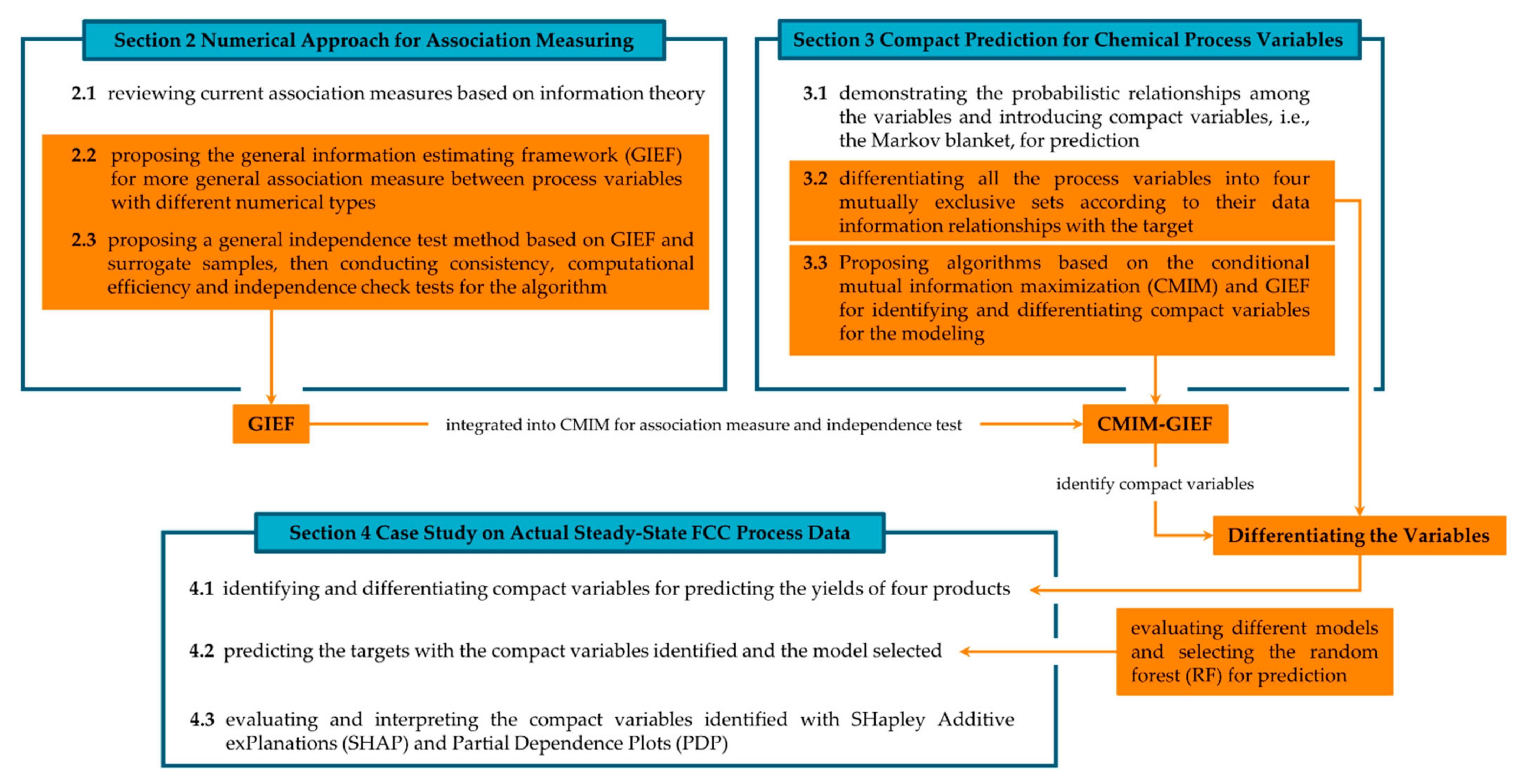
2. Data Predictability and Numerical Approach for Information Estimation

The essence of data-driven prediction lies in finding a subset of variables ${\mathcal{X}}^{\prime }=\left\{X_1,\cdots ,X_d\right\}$ in the full set $\mathcal{X}$ such that the posterior distribution of the target given ${\mathcal{X}}^{\prime }$, $P\left(Y|{\mathcal{X}}^{\prime }\right)$, will differ from the prior $P\left(Y\right)$ [44,45]. If $Y$ is associated with some variable $X\in {\mathcal{X}}^{\prime }$, a more precise prediction for it can be achieved compared to merely speculating from $P\left(Y\right)$. That is, $\exists X=x, Y=y$ so that

$$P\left(Y=y|X=x\right)\ne P\left(Y=y\right)$$

(1)

which means the association between $X$ and $Y$ can lead to a more accurate prediction. Otherwise, if $X$ is independent of $Y,$ for $\forall x,y$,

$$P\left(Y=y|X=x\right)=P\left(Y=y\right)$$

(2)

and $X$ cannot provide a better prediction. Note that Equations (1) and (2) indicate feasibility, not accuracy, while the latter characteristic is of more interest in industrial applications, which can further indicate association strengths between the variables and targets and imply the potential in the data for the prediction, i.e., predictability [44,45,46]. In statistics, the predictability of $X$ for $Y$ can be measured with MI, i.e., $I\left(Y;X\right)$ [47,48], which can be regarded as the sum of the logarithmic differences between the prior and posterior distributions of $Y$, i.e., $P\left(Y\right)$ and $P\left(Y|X\right)$, over the entire space. In this paper, the natural logarithm $\ln \left(·\right)$ is used for logarithmic operations because relevant conclusions in the later part of this section are obtained based on the natural logarithm [49,50]. If $X$ and $Y$ are both discrete,

$$\begin{array}{cc}\hfill I\left(X;Y\right)& ={\displaystyle {\displaystyle \sum }_{x,y\in \mathcal{X},\mathcal{Y}}}P\left(x,y\right)\left[\ln P\left(y|x\right)-\ln P\left(y\right)\right]\hfill \\ & ={\displaystyle {\displaystyle \sum }_{x,y\in \mathcal{X},\mathcal{Y}}}P\left(x,y\right)\ln \frac{P\left(x,y\right)}{P\left(x\right)P\left(y\right)}\hfill \end{array}$$

(3)

Similarly, if $X$ and $Y$ are both continuous,

$$I\left(X;Y\right)={{\displaystyle \iint }}_{x,y\in \mathcal{X},\mathcal{Y}}p\left(x,y\right)\ln \frac{p\left(x,y\right)}{p\left(x\right)p\left(y\right)}\mathrm{d}x\mathrm{d}y$$

(4)

where $\mathcal{X}$ and $\mathcal{Y}$ are the sets of all possible values; $P\left(x\right)$ and $P\left(y\right)$ are the probabilities at $X=x$ and $Y=y$; $p\left(x\right)$ and $p\left(y\right)$ are the probability densities.

MI can also be decomposed into combinations of marginal entropies $H\left(X\right)$, $H\left(Y\right)$ and joint entropies $H\left(X,Y\right)$ [48] in Equation (5):

$$I\left(X;Y\right)=H\left(X\right)+H\left(Y\right)-H\left(X,Y\right)$$

(5)

For discrete $X$ and $Y$,

$$H\left(X\right)=-{\displaystyle \sum }_{x\in \mathcal{X}}P\left(x\right)\ln P\left(x\right),H\left(Y\right)=-{\displaystyle \sum }_{y\in \mathcal{Y}}P\left(y\right)\ln P\left(y\right)$$

(6)

and for continuous $X$ and $Y$,

$$H\left(X\right)=-\underset{x\in \mathcal{X}}{{\displaystyle \int }}p\left(x\right)\ln p\left(x\right)\mathrm{d}x,H\left(Y\right)=-\underset{y\in \mathcal{Y}}{{\displaystyle \int }}p\left(y\right)\ln p\left(y\right)\mathrm{d}y$$

(7)

2.1. Numerical Approaches for Estimating Marginal Entropy and MI

Compared with classical statistical measurements such as Pearson’s and Spearman’s coefficients which have strict application prerequisites (e.g., types of distributions and monotonic linearity of data), marginal entropy and MI provides a non-parametric way to quantify arbitrary associations between nonlinear and nonnormal data [7,13,38,51]. Besides, these data-information-based metrics also have elegant and rigorous mathematical properties that make them applicable for bivariate or multivariate analysis. (Please see Equations (A1)–(A15) in Appendix A for more details and proofs.) However, despite easy prerequisites, the accuracy of the above data-information methods can still be affected by factors such as variable numerical types and varying sample sizes. Few studies have paid attention to such underlying computational details when applying the methods to chemical process data. For example, some process variables, such as temperature and pressure, are continuous, since their values are numerically comparable. While other variables closely related to process operations, such as the on-off states of valves, pumps, and wind blowers, are discrete since their values show no order and are incomparable. A chemical process typically consists of numerous continuous and discrete variables, which may lead to estimating entropies, MI, and conditional MI (CMI) for or between variables of different value types. Besides, it often involves concatenating multiple low-dimensional variables $X$ and $Y$ into the high-dimensional variable $\left(X, Y\right)$ to estimate the joint entropy $H\left(X,Y\right)$. Equations (3), (4), (6) and (7) and Equations (A1)–(A4) in Appendix A have demonstrated that continuous and discrete variables cannot be treated as the same type of value when computing the above metrics. Only the variables of the same type can be directly concatenated; otherwise, the type of the concatenated variable may be ambiguous.

If both $X$ and $Y$ are discrete, the estimated probabilities $\widehat{P}\left(x\right)$, $\widehat{P}\left(y\right)$ and $\widehat{P}\left(x,y\right)$ can be directly obtained by the sample frequencies, then taken into Equations (3), (6) and (A12) to get the estimates ${\widehat{H}}_{\mathrm{discrete}}\left(X\right)$, ${\widehat{H}}_{\mathrm{discrete}}\left(Y\right)$, ${\widehat{I}}_{\mathrm{discrete}}\left(X;Y\right)$ and ${\widehat{I}}_{\mathrm{discrete}}\left(X;Y|Z\right)$. However, if at least one of $X$ or $Y$ is continuous, common approaches using data quantization [44,52,53] to transform continuous variables into discrete may cause significant errors [42,50,54]. To solve this problem, Kozachenko and Leonenko [49] and Singh [55] et al. first proposed a classical KL entropy estimator based on the k-nearest neighbors:

$${\widehat{H}}_{\mathrm{KL}}\left(X\right)=\psi \left(N\right)-\psi \left(k\right)+\ln c_d+\frac{d}{N}{\displaystyle \sum }_{i=1}^N\ln {\epsilon }_i$$

(8)

where $N$ denotes the sample size; $k$ is the number of nearest neighbors; $\psi$ denotes the digamma function; $c_d$ denotes the volume of a unit ball in the $d$ dimensional space of $X$; and ${\epsilon }_i$ is the distance of the $i^{\mathrm{th}}$ sample to its $k^{\mathrm{th}}$ nearest neighbor. Note that the value of $c_d$ is related to the spatial distance metric selected. For example, when taking the maximum norm $L_{\infty }$, i.e., the Chebyshev distance, $c_d=2^d$; and when taking the $L_2$ norm, i.e., the Euclidean distance, $c_d={\pi }^{d/2}/\mathsf{\Gamma }\left(1+d/2\right)$ and $\mathsf{\Gamma }$ denotes the gamma function [54]. Studies show that the Euclidean distance generally applies to low-dimensional rather than high-dimensional data [56,57]. Based on the KL entropy estimator, Kraskov [50], Ross [42], Lombardi [54], Lord et al. [58], further proposed more accurate estimation approaches for mixed types of variables.

If both $X$ and $Y$ are continuous, Kraskov proposed computing the marginal and joint entropies of $X$ and $Y$ with adaptive $k$ and replacing the Euclidean distance with the Chebyshev distance to offset the bias caused by the scale differences between the marginal and joint spaces [50]. Kraskov’s estimate is shown in Equation (9) below:

$${\widehat{I}}_{\mathrm{Kraskov}}\left(X;Y\right)=\psi \left(N\right)+\psi \left(k\right)-\frac{1}{N}{\displaystyle \sum }_{i=1}^N\psi \left(n_{X,i}\right)+\psi \left(n_{Y,i}\right)$$

(9)

where $n_{X,i}$ is the number of neighbors that lie within the range of $x_i\pm {\epsilon }_i/2$. Furthermore, if one of $X$ and $Y$, say $X$, is discrete, Ross et al. [42] proposed the following MI estimate in Equation (10):

$${\widehat{I}}_{\mathrm{Ross}}\left(X;Y\right)=\psi \left(N\right)+\psi \left(k\right)-\frac{1}{N}{\displaystyle \sum }_{i=1}^N\psi \left(N_{X,i}\right)-\frac{1}{N}{\displaystyle \sum }_{i=1}^N\psi \left(n_i\right)$$

(10)

where $N_{X,i}$ denotes the number of samples with the same Y value as sample i.

2.2. GIEF: A General Framework for Data Information Estimation

The above Equations (3), (6) and (8)–(10) have achieved accurate estimations for marginal entropies and MI between variables of all value types. Further, some research areas in chemical processes such as causality analysis [19,59,60] and time-delayed causal analysis [40], often involve estimating conditional entropy and CMI to get transfer entropy and other metrics between multiple variables. So, this section will realize relevant algorithms and integrate them into the general information estimation framework (GIEF) proposed by the paper. For the convenience of later discussion, the marginal entropy estimations in Equations (6) and (8) is unified as H-GIEF, with the result denoted as ${\widehat{H}}_{\mathrm{g}}\left(X\right)$; MI estimates in Equations (3), (9) and (10) is unified as MI-GIEF, with the result as ${\widehat{I}}_{\mathrm{g}}\left(X;Y\right)$.

According to Equation (A5), the estimation for conditional entropy can be realized as

$${\widehat{H}}_{\mathrm{g}}\left(X|Z\right)={\widehat{H}}_{\mathrm{g}}\left(X\right)-{\widehat{I}}_{\mathrm{g}}\left(X;Z\right)$$

(11)

where ${\widehat{H}}_{\mathrm{g}}\left(X\right)$ and ${\widehat{I}}_{\mathrm{g}}\left(X;Z\right)$ can be obtained by former Equations (3), (6) and (8)–(10). It may be more difficult, however, to estimate CMI. If the conditional variable $Z$ is of the same type as $X$ or $Y$, say $Y$, then $Z$ and $Y$ can be concatenated into a new variable. Thus, CMI can be estimated by Equation (A7):

$${\widehat{I}}_{\mathrm{g}}\left(X;Y|Z\right)={\widehat{I}}_{\mathrm{g}}\left(Y,Z;X\right)-{\widehat{I}}_{\mathrm{g}}\left(X;Z\right)$$

(12)

Suppose Z is not of the same type as X and Y (implying that X and Y are in the same type). In this case, CMI can be estimated by Equation (A8) or (A9). Note that, although these two equations are mathematically equivalent, the former will have higher computational efficiency by avoiding the estimation of $H\left(Z\right)$.

$$\begin{array}{c}{\widehat{I}}_{\mathrm{g}}\left(X;Y|Z\right)={\widehat{I}}_{\mathrm{g}}\left(X;Y\right)+{\widehat{I}}_{\mathrm{g}}\left(X,Y;Z\right)-{\widehat{I}}_{\mathrm{g}}\left(X;Z\right)-{\widehat{I}}_{\mathrm{g}}\left(Y;Z\right)\\ ={\widehat{I}}_{\mathrm{g}}\left(X;Y\right)+{\widehat{H}}_{\mathrm{g}}\left(Z|X\right)+{\widehat{H}}_{\mathrm{g}}\left(Z|Y\right)-{\widehat{H}}_{\mathrm{g}}\left(Z|X,Y\right)-{\widehat{H}}_{\mathrm{g}}\left(Z\right)\end{array}$$

(13)

According to the above discussion, this paper puts forward a general approach for estimating the four data-information metrics: marginal entropy, conditional entropy, MI and CMI, as shown in Figure 2 below, which corresponds to the first part of the general information estimation framework (GIEF) proposed in this paper. It first calculates the marginal entropy estimate ${\widehat{H}}_{\mathrm{g}}\left(X\right)$ for continuous or discrete $X$ with Equations (6) and (8), respectively, then obtains the MI estimate ${\widehat{I}}_{\mathrm{g}}\left(X;Y\right)$ with Equations (3), (9) and (10), finally gets the estimates ${\widehat{H}}_{\mathrm{g}}\left(X|Z\right)$ and ${\widehat{I}}_{\mathrm{g}}\left(X;Y|Z\right)$ for condition entropy and CMI, respectively. The approach is applicable to both continuous and discrete variables in chemical processes.

2.3. Performance Tests for GIEF and Other Association Measuring Methods

The complex mechanisms in chemical processes can result in various forms of data relations and associations, coupled with significant differences in sample sizes. Hence, association analysis algorithms applied to studies should consistently quantify arbitrary linear and nonlinear associations with different distribution types and sample sizes. According to the test framework proposed by Kinney et al. [61], this section first conducts consistency and time cost tests for common association measuring approaches in chemical processes, such as PearsonCorr, distance correlation coefficient (DistCorr), SpearmanCorr and MI. Especially for estimating MI, four methods will be adopted: isometric quantization, iso-frequency quantization, adaptive quantization proposed by Darbellay et al. [53] and GIEF proposed in this paper, which are denoted as MI-cut, MI-qcut, MI-Darbellay and MI-GIEF, respectively.

2.3.1. Consistency and Time Costs

Figure S1 in the Supplementary Materials presents association values measured by different methods for 16 types of data relations (please refer to [61] for more dataset details). For each relation, the coefficients measured at different noise levels $1-{\mathrm{R}}^2$ are plotted by fixing $x$ and adding uniform noises on $y$. As the color varies from blue to red, the data linearity and monotonicity become gradually stronger. As Figure S1 illustrates, classical measures such as PearsonCorr, SpearmanCorr and DistCorr have obvious biases for different relations. They get higher coefficient values on linear or monotonic data but fail to detect nonlinearities. For the other four MI methods, only MI-qcut and MI-GIEF can achieve consistent results under a large sample size $N=2000$, with highly overlapped result points in each plot. Note, though, that as $N$ increases, the coefficient of MI-qcut on irrelevant data (where $1-{\mathrm{R}}^2$ equals to 0) deviates from 0 and becomes positive, which is inappropriate for use. Finally, only MI-GIEF achieves consistent measurements on all the data with $N \ge 2000$. Besides, Figure S2 shows variations of average computational time costs obtained by different methods in Figure S1 and the corresponding 95% confidence intervals (CIs) with increasing sample sizes. Combining Figures S1 and S2 suggests that MI-GIEF can obtain more accurate estimates than other MI methods with comparable time costs as DistCorr and MI-Darbellay’s. The algorithm can be further optimized in the future to improve its accuracy and computational efficiency.

2.3.2. Test of Independence in GIEF

The independence test aims to determine whether the variables are independent or conditionally independent from the vantage of statistical significance, and identify hidden associations from a large amount of data. It is an essential topic in statistical analysis and facilitates data dimensionality reduction, process modeling, causal analysis, and identification of control variables in industrial practices [30,31,62]. Compared to traditional linear metrics such as PearsonCorr and SpearmanCorr, MI can detect arbitrary (linear or nonlinear) associations and conditional associations [7,61,63]. Although, compared with quantization-based methods, MI-GIEF and CMI-GIEF can achieve more accurate and stable estimations for mixed-type data [42], studies show that their results are also susceptible to data noise, sample size and association forms [64,65]. This section will propose more accurate independence and conditional independence tests and integrate them into the GIEF framework as the second part.

Figure A1 in Appendix B illustrates that the means and variances of the MI-GIEF estimates can be significantly affected by sample size $N$; the fluctuations in ${\widehat{I}}_{\mathrm{g}}\left(X;Y\right)$ decrease with increasing $N$. Thus, discriminating independence and association based on a fixed threshold of the estimate is not suitable for different data distributions and sample sizes; otherwise, it will cause high rates of Type I errors [62]. So it is necessary to propose more accurate and general independence tests that are less affected by data distributions and sample sizes. This paper will consider the surrogate independence test, which has been proven to be adaptive to varying sample sizes [52,62]. First, the method will randomly construct a set of surrogate samples ${\mathcal{D}}_{\mathrm{surrog}}=\left\{\left(x_1^{\mathrm{s}},y_1\right),\left(x_2^{\mathrm{s}},y_2\right),\dots ,\left(x_N^{\mathrm{s}},y_N\right)\right\}$ from the original set $\mathcal{D}=\left\{\left(x_1,y_1\right),\left(x_2,y_2\right),\dots ,\left(x_N,y_N\right)\right\}$, where the superscript $\mathrm{s}$ denotes the randomly shuffled indexes of $X$. Then, it will estimate ${\widehat{I}}_{\mathrm{g}}\left(x^{\mathrm{s}};y\right)$ for all the surrogate samples and obtain the distribution corresponding to the null hypothesis denoted as $H_0$. The method will finally check whether ${\widehat{I}}_{\mathrm{g}}\left(x;y\right)$ is in the distribution of $H_0$: if P is greater than significance level $\alpha$, accept $H_0$, i.e., reject independence; otherwise, accept $H_1$, i.e., accept independence. Based on the above discussion, this paper proposes the algorithm CheckIndep in Table S1, which composes the second part of the GIEF framework.

Table 1. Detection rates of independence with GIEF.

Dataset	Description	$\mathit{N}=100$	$\mathit{N}=1000$
random	$y~\mathrm{Uniform}\left(0, 1\right)$	0.94 (0.92, 0.96)	0.94 (0.93, 0.96)
linear	$y=x+\epsilon$	0 (0, 0)	0 (0, 0)
parabola	$y=4x^2+\epsilon$	0 (0, 0)	0 (0, 0)
categorical	$y=\left\{\begin{array}{l}0.287+\epsilon , \mathrm{if} x=0.25\\ 0.796+\epsilon , \mathrm{if} x=0.5\\ 0.290+\epsilon , \mathrm{if} x=0.75\\ 0.924+\epsilon , \mathrm{if} x=1\end{array}\right.$	0 (0, 0)	0 (0, 0)

below shows the effects of CheckIndep on the datasets in Figure A1. The data of $X$ in the top three datasets (random, linear and parabola) are randomly sampled from the uniform distribution: $x~\mathrm{Uniform}\left(0, 1\right)$. In the last dataset (categorical), $x$ is sampled from $\left\{0.25, 0.5, 0.75, 1\right\}$ with equal probability. The data of $Y$ are obtained as described in the table, where $\epsilon$ is the uniform noise imposed: $\epsilon ~\mathrm{Uniform}\left(0, 0.01\right)$. Each test is repeated for 100 rounds, and the results are denoted in the format as $median, \left(q_1, q_3\right)$, corresponding to the median, lower and upper quantiles of percentages that accept independence. The results of the random dataset show that when $N$ are set to 100 and 1000, the surrogate-data method can identify all the independence relations with rates equal to 94%. As for the other three datasets, the surrogate-data method identifies all the associations accurately.

Table 2. Detection rates of conditional independence with GIEF.

Dataset	Description	$\mathit{N}=100$	$\mathit{N}=1000$
M1	$x=\tilde{x}+z+{\epsilon }_x$ $y=\tilde{y}+z+{\epsilon }_y$	0.96 (0.95, 0.98)	0.94 (0.92, 0.95)
M2	$x=\tilde{x}+z+{\epsilon }_x$ $y=z^2+{\epsilon }_y$	0.92 (0.90, 0.93)	0.92 (0.91, 0.94)
M3	$x=\tilde{x}+z+{\epsilon }_x$ $y=0.5·\sin \left(\pi \tilde{x}\right)+{\epsilon }_y$	0 (0, 0)	0 (0, 0)
M4	$x=\tilde{x}+z+{\epsilon }_x$ $y=\tilde{x}+\tilde{y}+z+{\epsilon }_y$	0 (0, 0)	0 (0, 0)

below lists the results of conditional independence tests with GIEF for datasets M1 to M4. Samples $\tilde{x},\tilde{y}$ and $\tilde{z}$ are drawn from the standard normal distribution independently. Values ${\epsilon }_x$ and ${\epsilon }_y$ are uniform noises imposed on the outputs. It is easy to check that conditional independence $\left(X\perp Y|Z\right)$ holds for M1 and M2, which is confirmed by the test results.

In summary, Section 2 proposes and tests a general framework GIEF for estimating information entropy, conditional entropy, MI and CMI and independence tests for or between arbitrary types of variables, one which is applicable for chemical processes and will be the basis for the later part of this paper.

3. Compact Prediction for Chemical Process Data Based on Association Measure, Independence Test and Probabilistic Graph

3.1. Compact Variables Set and the Markov Blanket

Due to nonlinear mechanisms and complex material flows, chemical process variables often exhibit complex data-information relations. For example, sometimes multiple sensors may be placed together to precisely measure an important variable $X$ (such as the sensitive plate temperature, reactor temperature, and pressure in distillation columns) for predicting a key outcome $Y$ (such as product yield). Assume the measured signals are denoted as $X_1$, $X_2$ and $X_3$, and their data should be highly linearly correlated so that $X_i\approx X_1$ for $2\le i\le 3$. According to Equation (A14), $I\left(X_i;Y|X_1\right)=0$, so that $I\left(X_1,X_2,X_3;Y\right)=I\left(X_1;Y\right)$, which indicates repeating measurements for the same variable is redundant for prediction. Since $X_2$ and $X_3$ are linearly correlated with $X_1$, such redundancy can be removed through multicollinearity analysis [66,67]. In other situations, sometimes series connections of devices via pipelines can link $X_1$, $X_2$, $X_3$ and $Y$ as a Markov chain: $X_1\to X_2\to X_3\to Y$, so that the variation of $Y$ depends only on $X_3$ and is independent of upper-stream $X_1$ and $X_2$, so that $I\left(X_i;Y|X_3\right)=0$ for $1\le i\le 2$. In this case, only $X_3$ should be kept, while $X_1$ and $X_2$ are redundant for $Y$. In this circumstance, due to potentially nonlinear process mechanisms, $X_1$ and $X_2$ may not be linearly correlated with $X_3$, and multicollinearity analysis may fail to exclude the redundancy effectively.

The above-mentioned repeated measurements and information transfer Markov chains are typical chemical process phenomena related to data redundancy and irrelevancy. Actually, the relations between different process variables can be more complex, which can be described by the Bayesian network ${\mathcal{G}}^{\mathrm{B}}$ in Figure 3a [9,68,69,70]. The nodes of ${\mathcal{G}}^{\mathrm{B}}$ correspond to process variables, and the arrows denote causal connections. For a target $Y$, its parents, children and spouses are denoted as ${\mathcal{X}}^{\mathrm{p}}$ (corresponding to $X_1^{\mathrm{p}}$, $X_2^{\mathrm{p}}$ and $X_3^{\mathrm{p}}$ in the figure), ${\mathcal{X}}^{\mathrm{c}}$ ($X_1^{\mathrm{c}}$ and $X_2^{\mathrm{c}}$) and ${\mathcal{X}}^{\mathrm{s}}$ ($X_1^{\mathrm{s}}$), respectively. It is easy to see that $Y$ is directly connected with ${\mathcal{X}}^{\mathrm{p}}$, ${\mathcal{X}}^{\mathrm{c}}$ and indirectly connected with ${\mathcal{X}}^{\mathrm{s}}$ and other remaining nodes ${\mathcal{X}}^{\mathrm{r}}=\mathcal{X}\backslash \left({\mathcal{X}}^{\mathrm{p}}\cup {\mathcal{X}}^{\mathrm{c}}\cup {\mathcal{X}}^{\mathrm{s}}\right)$.

According to the $d$-separation theorem [51], for a target $Y$ in ${\mathcal{G}}^{\mathrm{B}}$, its parents ${\mathcal{X}}^{\mathrm{p}}$, children ${\mathcal{X}}^{\mathrm{c}}$ and spouses ${\mathcal{X}}^{\mathrm{s}}$ together block the effects of other process variables transmitted to it. In other words, $Y$ is conditionally independent of all the remaining nodes $\mathcal{X}\backslash \left({\mathcal{X}}^{\mathrm{p}}\cup {\mathcal{X}}^{\mathrm{c}}\cup {\mathcal{X}}^{\mathrm{s}}\right)$ given ${\mathcal{X}}^{\mathrm{p}}$, ${\mathcal{X}}^{\mathrm{c}}$ and ${\mathcal{X}}^{\mathrm{s}}$, that is,

$$I\left(Y;{\mathcal{X}}^{\mathrm{r}}|{\mathcal{X}}^{\mathrm{p}},{\mathcal{X}}^{\mathrm{c}},{\mathcal{X}}^{\mathrm{s}}\right)=0$$

(14)

In this way, ${\mathcal{X}}^{\mathrm{p}}$, ${\mathcal{X}}^{\mathrm{c}}$ and ${\mathcal{X}}^{\mathrm{s}}$ can be considered as a whole, i.e., the Markov blanket (MB) of $Y$, which is the union of ${\mathcal{X}}^{\mathrm{p}}$, ${\mathcal{X}}^{\mathrm{c}}$ and ${\mathcal{X}}^{\mathrm{s}}$ in the Bayesian network ${\mathcal{G}}^{\mathrm{B}}$ [30,51,71]:

$${\mathcal{M}}_Y={\mathcal{X}}^{\mathrm{p}}\cup {\mathcal{X}}^{\mathrm{c}}\cup {\mathcal{X}}^{\mathrm{s}}$$

(15)

Then Equation (14) can be re-written to Equation (16), which demonstrates the information-blocking nature of MB:

$$I\left(Y;\mathcal{X}\backslash {\mathcal{M}}_Y|{\mathcal{M}}_Y\right)=0$$

(16)

The paper also finds that the MB variables are irreplaceable for prediction; otherwise, it will lead to unavoidable data information loss and prediction accuracy decrease, as illustrated in the following Equation (17). For any non-empty subset ${\mathcal{M}}^{\prime }\subset {\mathcal{M}}_Y$, the information in ${\mathcal{M}}^{\prime }$ about $Y$ will not be blocked by the other nodes in MB, ${\mathcal{M}}_Y\backslash {\mathcal{M}}^{\prime }$, so that $I\left(Y;{\mathcal{M}}^{\prime }|{\mathcal{M}}_Y\backslash {\mathcal{M}}^{\prime }\right)>0$. At the same time, $I\left(Y;{\mathcal{M}}_Y\right)=I\left(Y;{\mathcal{M}}_Y\backslash {\mathcal{M}}^{\prime }\right)+I\left(Y;{\mathcal{M}}^{\prime }|{\mathcal{M}}_Y\backslash {\mathcal{M}}^{\prime }\right)$ and $I\left(Y;{\mathcal{M}}_Y\right)>0$, so that

$$I\left(Y;{\mathcal{M}}_Y\backslash {\mathcal{M}}^{\prime }\right)<I\left(Y;{\mathcal{M}}_Y\right), \forall {\mathcal{M}}^{\prime }\subset {\mathcal{M}}_Y$$

(17)

Combining the above Equations (16) and (17) demonstrates that MB contains sufficient information for the prediction without redundancy and irrelevancy, implying that it is the compact set of associated variables for $Y$.

3.2. Variable Differentiation from the Information-Theoretic Perspective

Section 3.1 shows that a sufficiently accurate and compact prediction depends on precisely identifying MB in ${\mathcal{G}}^{\mathrm{B}}$, which is composed of parents, children and spouses of the target. Note that the parents and children are directly associated with the target, while some spouses are conditionally associated [30]. Due to the data information transmission discussed in Section 3.1, some variables outside MB may also be associated with the target. Therefore, the independence test algorithm CheckIndep proposed in Section 2.3.2 and Table S1 cannot directly identify MB [31] without further defining and differentiating various types of variables. In addition, in industrial applications, accurately identifying the directly associated variables (i.e., parents and children) can help eliminate redundancy and irrelevancy in the data and discriminate the direct causes and effects of the target [30,72], thus guiding the construction of local causal networks [31], which will be our future work.

This paper first realizes the identification of MB from the data information perspective and then differentiates the types of variables in and out of MB to determine the compact and directly associated variables of the target. Recent studies have defined several association relations, e.g., strong and redundant associations, in different forms [43,73,74,75], but there is still no unified way for numerical computations. Therefore, this paper redefines all the association relations in the forms of MI and CMI and unifies the calculation procedures into the independence tests based on GIEF in Table S1, which will facilitate more convenient calculations. Different sets of variables are defined as follows:

• Strongly associated variables ${\mathcal{X}}^{\mathrm{sa}}$: if a variable node $X_i$ is directly connected to $Y$ on ${\mathcal{G}}^{\mathrm{B}}$ and cannot be blocked by any other node sets ${\mathcal{X}}^{\prime }\subseteq \mathcal{X}\backslash \left\{X_i\right\}$, then $X_i\in {\mathcal{X}}^{\mathrm{sa}}$ is strongly associated with $Y$, that is, for $\forall {\mathcal{X}}^{\prime }\subseteq \mathcal{X}\backslash \left\{X_i\right\}$, $I\left(X_i;Y|{\mathcal{X}}^{\prime }\right)>0$;
• Interactively associated variables ${\mathcal{X}}^{\mathrm{ia}}$: if a node $X_i$ is not directly connected to $Y$ on ${\mathcal{G}}^{\mathrm{B}}$ but conditionally associated with $Y$ given nodes set ${\mathcal{X}}^{\prime }\subseteq \mathcal{X}\backslash \left\{X_i\right\}$, then $X_i\in {\mathcal{X}}^{\mathrm{ia}}$ is interactively associated with $Y$, that is, $I\left(X_i;Y\right)=0$ and $\exists {\mathcal{X}}^{\prime }\subseteq \mathcal{X}\backslash \left\{X_i\right\}$ so that $I\left(X_i;Y|{\mathcal{X}}^{\prime }\right)>0$;
• Redundantly associated variables ${\mathcal{X}}^{\mathrm{ra}}$: if a node $X_i$ is associated with $Y$ but conditionally independent of $Y$ given some nodes ${\mathcal{X}}^{\prime }\subseteq \mathcal{X}\backslash \left\{X_i\right\}$, then $X_i\in {\mathcal{X}}^{\mathrm{ra}}$ is called a redundant associated variable for $Y$, that is, $I\left(X_i;Y\right)>0$ and $\exists {\mathcal{X}}^{\prime }\subseteq \mathcal{X}\backslash \left\{X_i\right\}$ so that $I\left(X_i;Y|{\mathcal{X}}^{\prime }\right)=0$;
• Irrelevant variables ${\mathcal{X}}^{\mathrm{ir}}$: if a node $X_i$ is neither associated nor conditionally associated with $Y$ given any subset ${\mathcal{X}}^{\prime }\subseteq \mathcal{X}\backslash \left\{X_i\right\}$, then $X_i\in {\mathcal{X}}^{\mathrm{ir}}$ is called completely irrelevant to $Y$, that is, for $\forall {\mathcal{X}}^{\prime }\subseteq \mathcal{X}\backslash \left\{X_i\right\}$, $I\left(X_i;Y|{\mathcal{X}}^{\prime }\right)=0$.

Based on the above definitions, Figure 4 below provides a variable differentiation flowsheet that separates all the variables into four mutually exclusive sets:

$$\mathcal{X}={\mathcal{X}}^{\mathrm{sa}}\cup {\mathcal{X}}^{\mathrm{ia}}\cup {\mathcal{X}}^{\mathrm{ra}}\cup {\mathcal{X}}^{\mathrm{ir}}$$

(18)

According to the probabilistic graph theory [30,51], the above four types of relations correspond to different types of nodes in the Bayesian network in Figure 3b, where the strongly associated variables correspond to the combination of parents and children, as they are directly connected to $Y$: ${\mathcal{X}}^{\mathrm{sa}}={\mathcal{X}}^{\mathrm{p}}\cup {\mathcal{X}}^{\mathrm{c}}$; the interactively associated variables correspond to spouses, ${\mathcal{X}}^{\mathrm{ia}}={\mathcal{X}}^{\mathrm{s}}$, as they are indirectly connected with $Y$ via colliders; the redundantly associated variables correspond to the nodes associated with $Y$ but blocked by ${\mathcal{X}}^{\mathrm{sa}}$ and ${\mathcal{X}}^{\mathrm{ia}}$; and the irrelevant variables correspond to the remaining nodes in the network, which are not associated or conditionally associated with $Y$. In addition, according to Figure 3 and Equation (15), ${\mathcal{X}}^{\mathrm{sa}}$ and ${\mathcal{X}}^{\mathrm{ia}}$ constitute the compact association variables, i.e., the MB, of $Y$, and ${\mathcal{X}}^{\mathrm{sa}}$ contains all the direct causes and effects.

Figure 4 also implies that differentiating variables based on pairwise single-factor methods (for example, measuring direct associations by PearsonCorr, SpearmanCorr and MI) are inadequate for identifying compact variables. As shown by the first step in the figure, the methods may probably keep redundant variables and exclude interactively associated variables, which will increase the model’s dimensionality and lose essential predictive information, making it more likely for the model to encounter the curse of dimension problem under limited samples [24]. In the next section, relevant algorithms based on GIEF will be proposed to identify compact associated variables and differentiate them according to the above definitions from the information-theoretic perspective.

3.3. Algorithms for Identifying and Differentiating Compact Variables in Chemical Processes

According to the analysis in Section 3.1 and Section 3.2, this section first considers identifying MB from the information-theoretic perspective. It supposes that the process variables that can provide additional data information about the target should be iteratively selected into the Markov blanket set ${\mathcal{M}}_Y$, until the total MI value $I\left({\mathcal{M}}_Y;Y\right)$ reaches maximum. According to this principle, an incremental feature selection procedure called Conditional Mutual Information Maximization (CMIM) [43,73] is adopted for study (please see Equations (A16)–(A23) in Appendix C for detailed derivations). Note that, in this paper, the algorithm will be realized as Equation (19) based on GIEF, where the CMI estimate ${\widehat{I}}_{\mathrm{g}}\left(f;Y|r\right)$ is supposed to be more accurate and reliable for chemical process data. Table S2 presents a detailed flowsheet for identifying MB step by step with GIEF, which is named CMIM-GIEF and the final result $\mathcal{S}$ corresponds to MB, ${\mathcal{M}}_Y$. As a comparison, the CMIM realized by CMI with iso-frequency quantization is named CMIM-Q. The effects of CMIM-GIEF and CMIM-Q will be compared with other methods later in Section 4.

$$S^{\left(t\right)}=\underset{f\in \mathcal{F}-{\mathcal{S}}^{\left(t-1\right)}}{\arg \max }\left\{\underset{r\in {\mathcal{R}}^{\left(t\right)}}{\min }{\widehat{I}}_{\mathrm{g}}\left(f;Y|r\right)\right\}$$

(19)

After CMIM-GIEF, the flowsheet in Figure 4 and algorithms CheckIndep proposed in Section 2.3.2 are combined to further differentiate the MB and non-MB variables according to their associations with the target. The corresponding algorithm DifferentiateVariables is proposed in Table S3. In summary, this section has completed the data-information-based algorithms for identifying compact associated variables and differentiating their data-information relations with the target. The next section will apply and evaluate the effects of these algorithms on actual FCC process steady-state data for predicting the yields of some important products.

4. Case Study on Actual Steady-State FCC Process Data

The FCC process is one of the most important conversion processes in the petrochemical industry. It mainly uses high-temperature thermal cracking reactions with catalysts to convert high-boiling-point and high-molecular-weight hydrocarbon components in crude oil into valuable products such as gasoline and diesel. The process is highly complex due to nonlinear mechanisms, intricate flows, and numerous variables. Real-time prediction for steady-state FCC product yields is challenging and can provide powerful guidance for reactor design, product property prediction, operation optimization and catalyst selection. Besides, it can also provide more profound knowledge and understanding of reaction mechanisms, further promoting the development of process technology. However, due to the highly coupled reactions and complex variable relations, it is not easy to build models for the process. This paper attempts to use data-driven approaches to achieve regressive predictions for the yields of four critical products: light diesel (LD), heavy diesel (HD), gasoline (GAS), and dry gas (DG). A total number of $N=2727$ steady-state samples from July 2016 to May 2017 are collected for the study, which contain 217 continuous and discrete variables and 4 continuous product yields in the reaction-regeneration and fractionation systems, as shown in Figure S3, in which the four product flows are marked as blue lines and the variables of temperature (T), flow (F), pressure (P), liquid level (L), density (D), and analytical data (A) account for 38%, 27%, 19%, 10%, 5%, and 1% of the total, respectively. The variables and targets are highly coupled with complex relations.

In this section, the algorithms proposed in Section 3 ResolveMarkovBlanket and DifferentiateVariables will be applied to first identify the compact set of associated variables for the four yields, and then differentiate the variables according to their data-information relations with the targets. In the MB identification and variable differentiation steps, key variables associated with the targets are not set in advance by expert experience. The entire calculation is automatically executed based on data, which can better reflect and verify the data interactions. Machine-learning prediction models are also built with the compact associated variables identified. The prediction effects are evaluated, compared and interpreted.

4.1. Identifying Compact Associated Variables for the FCC Product Yields

All the steady-state samples are randomly partitioned into training and testing sets at a ratio of 7:3 for later compact variables identification, differentiation and predictive modeling. In this section, the MB and non-MB variables are first identified for the four yields $Y_{\mathrm{LD}}, Y_{\mathrm{HD}},Y_{\mathrm{GAS}}$ and $Y_{\mathrm{DG}}$ based on ResolveMarkovBlanket with CMIM-GIEF. Then, the variables are differentiated according to DifferentiateVariables.

Table 3. Sizes of MBs identified and the corresponding medians and quantiles of the MI-GIEF estimates.

Target	Variables in MB		Variables Not in MB		Total
-	Number	Distribution of MI	Number	Distribution of MI	Number	Distribution of MI
$Y_{\mathrm{LD}}$	25	0.701 (0.569, 0.808)	192	0.447 (0.303, 0.584)	217	0.476 (0.338, 0.615)
$Y_{\mathrm{HD}}$	23	0.890 (0.787, 1.000)	194	0.549 (0.373, 0.744)	217	0.583 (0.408, 0.773)
$Y_{\mathrm{GAS}}$	20	0.840 (0.707, 0.961)	197	0.526 (0.354, 0.692)	217	0.555 (0.382, 0.705)
$Y_{\mathrm{DG}}$	28	0.520 (0.409, 0.598)	189	0.313 (0.222, 0.403)	217	0.340 (0.231, 0.439)

and Figure 5a show the Markov blankets identified by CMIM-GIEF for the four targets, illustrating that the MB of each target contains significantly fewer variables than the total. The variables in MBs have significantly higher MI values and stronger associations with the targets, demonstrating the validity of the GIEF-based association measurement.

Figure 5a also illustrates that some variables can affect multiple targets simultaneously (e.g., the fifth variable in the figure, i.e., the temperature on the fresh feed nozzle of the lift tube in

Table 4. Variables information related to the product yields of the process in Figure 5b.

Variable Number	Variable Name	Note	Value Range	Targets Affected
5	TI-3107B	fresh material temperature in the lifting tube nozzle, °C	[401, 457]	$Y_{\mathrm{LD}},Y_{\mathrm{HD}},Y_{\mathrm{GAS}},Y_{\mathrm{DG}}$
24	TI-3112	outlet temperature of the settler, °C	[504, 514]	$Y_{\mathrm{DG}}$
26	TI-3117	temperature of the slide valve in the settler, °C	[499, 518]	$Y_{\mathrm{DG}}$
132	TI-3546	outlet temperature (A) of the evaporation section, °C	[391, 547]	$Y_{\mathrm{LD}},Y_{\mathrm{HD}},Y_{\mathrm{DG}}$
133	TI-3542	outlet temperature (B) of the evaporation section, °C	[127, 181]	$Y_{\mathrm{LD}},Y_{\mathrm{GAS}},Y_{\mathrm{DG}}$
134	TI-3551	outlet temperature of coal saver in the waste heat boiler, °C	[129, 192]	$Y_{\mathrm{GAS}},Y_{\mathrm{DG}}$
201	TI-3237	outlet temperature at the bottom of the stripper tower, °C	[136, 180]	$Y_{\mathrm{LD}},Y_{\mathrm{HD}},Y_{\mathrm{GAS}}$
13	FIC-3104	flowrate of refining slurry in the lift tube, t/h	[6, 35]	$Y_{\mathrm{HD}},Y_{\mathrm{GAS}},Y_{\mathrm{DG}}$
52	FIC-3118	flowrate of combustion oil in the first regenerator, m3/min	[0, 7]	$Y_{\mathrm{LD}},Y_{\mathrm{HD}}$
158	FIQ-3519	inlet flowrate (A) of fuel gas in the waste heat boiler, t/h	[0, 2717]	$Y_{\mathrm{LD}},Y_{\mathrm{HD}},Y_{\mathrm{DG}}$
159	FIQ-3520	inlet flowrate (B) of fuel gas in the waste heat boiler, t/h	[0, 1163]	$Y_{\mathrm{GAS}}$
194	FIC-3203	flowrate of oil slurry returning to the fractionation tower, t/h	[220, 407]	$Y_{\mathrm{HD}},Y_{\mathrm{GAS}},Y_{\mathrm{DG}}$
204	FIC-3223	steam flowrate (A) in the stripper tower, t/h	[1, 2]	$Y_{\mathrm{LD}}$
212	FIC-3403	steam flowrate (B) in the stripper tower, t/h	[16, 83]	$Y_{\mathrm{LD}},Y_{\mathrm{HD}},Y_{\mathrm{GAS}}$
71	PI-3114	main air pressure of the second regenerator, MPa	[0.27, 0.35]	$Y_{\mathrm{HD}}$

, affects all the yields), indicating the compact association network in Figure 5b, in which the red and white nodes denote the targets and variables with variable numbers and target names in the center of each node. The undirected edge between two nodes indicates the association relation, and the thickness corresponds to the MI value between them. The figure shows that there are stronger associations between $Y_{\mathrm{LD}}$, $Y_{\mathrm{HD}}$, and $Y_{\mathrm{GAS}}$ and their Markov blankets, implying better prediction effects for them. Table 4 lists the information of some important compact variables identified including material flow rates, temperatures and pressures in the lift tube, settler, waste heat boiler and stripper tower, which correspond to the variables presented in the figures in Section 4.3.

Table 5. Variable differentiation results.

Target	Strongly Associated	Interactively Associated	Redundantly Associated	Irrelevant	Total
$Y_{\mathrm{LD}}$	25	0	144	48	217
$Y_{\mathrm{HD}}$	23	0	151	43	217
$Y_{\mathrm{GAS}}$	20	0	157	40	217
$Y_{\mathrm{DG}}$	28	0	101	88	217

below shows the results of DifferentiateVariables, demonstrating that only a few variables are strongly associated with the yields, while the others are redundant or irrelevant. In addition, the algorithm does not find any interactively associated variables in this case, which is reasonable. Otherwise, if a variable is interactively associated with an outcome yield, there will be a collider between them according to Figure 3a. In this circumstance, the yield will cause the collider (a process variable), which rarely happens and is not detected.

In summary, with the algorithms proposed in Section 3, Section 4.1 has identified compact associated variables for the FCC product yields, which form a network structure. The variable differentiation results show that all the targets are only affected by small numbers of strongly associated variables. The accuracy and compactness of the results will be further verified in the next section.

4.2. Prediction Based on the Compact Associated Variables Identified

This section will use the results in Section 4.1 for building and testing machine-learning predictive models for the four yields to verify the accuracy and compactness of the associated variables identified. Since all the four targets are continuous, only regressive models are considered, and the metrics such as the determination coefficient R², mean absolute error (MAE), mean square error (MSE) and mean absolute percentage error (MAPE) are adopted for the model evaluation process [7,8,76]. First, five rounds of five-fold cross-validations are executed on the training dataset to examine and compare the prediction performance of different candidate machine-learning models, of which the random forest (RF) shows the overall best performance in R², MAE, MSE and MAPE, and is selected for the modeling in the later part of this paper [8,77,78]. Please refer to Table S4 in the Supplementary Materials for model evaluation details.

Table 6. Parameter settings for RF.

Parameter	Note	Value
criterion	the function to measure the quality of a split	“mse” 1
max_features	the number of features to consider when looking for the best split	“sqrt” 2
min_samples_split	the minimum number of samples required to split an internal node	10
min_samples_leaf	the minimum number of samples needed to be at a leaf node	3
n_estimators	the number of trees in the forest	100

¹ Mean square error, i.e., MSE. ² The number of features considered for split equals to the square root of the total number.

shows the parameter settings for RF obtained by the Grid Search strategy [7].

Next, the total and compact associated variables identified by CMIM-GIEF and CMIM-Q are used for building RF models, respectively. Meanwhile, other well-known methods frequently used in chemical processes, such as PearsonCorr [11], SpearmanCorr [10], DistCorr [11], MI [13,79], Mean Decrease Impurity (MDI) [80], Mean Decrease Accuracy (MDA) [81], Genetic Algorithm (GA) [8], Lasso [14], Ridge [15], Principal Component Analysis (PCA) [16], Kernal PCA (KPCA) [72,82], Locally Linear Embedding (LLE) [83] and Partial Least Square (PLS) [17], are also included in building the models. For each method, a hundred-round bootstrap test is performed. In each round, the model is first trained with the resampled data from the training set, and then the prediction metrics are obtained on the test set. Figure 6 and Table S5 show the number of variables (or features) and average metric values corresponding to the best model performance. Figure 7, Figure 8, Figure 9 and Figure 10 further exhibit the distributions of metric values on the four yields, where the circles within each box plot indicate mean values. From the comparison in Figure 6, the numbers of variables obtained by the feature selection methods except for CMIM-GIEF are significantly higher than those of the feature extraction methods. However, they achieve better predictions as shown in Table S5 and Figure 7, Figure 8, Figure 9 and Figure 10. Among these methods, CMIM-GIEF achieves the overall best prediction accuracies with minimal variables. It obtains the best results on $Y_{\mathrm{LD}}$ and $Y_{\mathrm{GAS}}$ and good results on $Y_{\mathrm{HD}}$ and $Y_{\mathrm{DG}}$ as well, results which are close to the optimal ones. In addition, comparing CMIM-GIEF and CMIM-Q shows that the former method achieves slightly better accuracies than the latter with fewer variables, which proves the effectiveness of GIEF in CMIM-GIEF for variable information estimation.

In summary, this section compares CMIM-GIEF, CMIM-Q and other well-known data dimensionality reduction methods for predicting the yields of four FCC products. The results show that CMIM-GIEF achieves the overall best prediction effects regarding model dimensionality and accuracy with the compact associated variables identified.

4.3. Evaluating and Interpreting the Compact Associated Variables Identified

Section 4.2 shows that the compact associated variables identified by CMIM-GIEF achieve the overall best dimensionality reduction results compared to other commonly used methods in chemical processes. This section will further analyze and interpret the results. In 2017, Lundberg and Lee proposed the Shapley Additive exPlanations (SHAP) method to explain various machine-learning classification and regression models [84], quantifying each feature’s linear and nonlinear impacts on the model predictions. The SHAP value of each feature $X_i$, $SHA{P}_i$, reflects the direction and strength of the impact on the target. $SHA{P}_i>0$ or $<0$ indicates that $X_i$ positively or negatively affects the target to obtain higher or lower values than the baseline level, which equals to the average predicted value over all the samples.

This section interprets the variables identified by CMIM-GIEF, and Figure 11 shows the summary plots and variable importance scores obtained by SHAP. The scatter-points in each row of the summary plot exhibit the SHAP values (horizontal coordinates) of $X_i$ in the test set. The higher the $X_i$ value is, the more red the point. Please see Table 4 for variables information. As a variable’s importance score decreases, the variable poses a weaker effect on the target, and this leads to a greater concentration of SHAP values at $SHA{P}_i=0$ in the plot.

Figure 12 also shows Partial Dependence Plots (PDP) obtained from the SHAP values for each target. In each plot corresponding to variable $X_i$ and target $Y_j$, the bold blue line indicates the PDP curve; the horizontal coordinates indicate the normalized variable values (please see Table 4 for the original value ranges); the vertical coordinates indicate the model outputs; the vertical dashed line indicates the expectation of $X_i$, $\mathrm{E}\left(X_i\right)$; and the horizontal dashed line indicates the expectation of the model outputs, $\mathrm{E}\left(f\left(X_i\right)\right)$. In addition, each PDP plot also shows the individual conditional expectation (ICE) curves, which are denoted as light-blue dashed lines. For each individual sample, its ICE curve is obtained by first randomly setting the values of $X_i$ while keeping other variables constant and then obtaining the relation between the expectation of the model outputs and $X_i$. Both the ICE and PDP curves in Figure 12 reflect the detailed effects of variables on the model outputs. As the importance scores of the variables decrease, the ICE and PDP curves become flattened.

The above analysis finds that the compact associated variables identified by CMIM-GIEF, such as outlet temperature TI-3107B in the riser tube, steam flow rates FIC-3223 and FIC-3403 in the stripper tower, outlet temperatures TI-3546 and TI-3551 and fuel gas flow rate FIQ-3520 in the waste heat boiler, do have significant impacts on the targets with different forms and degrees. For example, the temperature TI-3107B simultaneously affects $Y_{\mathrm{LD}}, Y_{\mathrm{HD}}$ and $Y_{\mathrm{GAS}}$, which has been reported in other studies and is adopted as a critical variable in process studies called the riser outlet temperature (ROT) [85,86]. In this case, higher values of TI-3107B will lead to higher values of $Y_{\mathrm{HD}}$ and lower values of $Y_{\mathrm{LD}}$. These complementary relations may be related to the diesel fraction blending process. The analysis also reveals that higher values of rise tube temperature TI-3107B and feed flowrate FIC-3203 can decrease the values of $Y_{\mathrm{GAS}}$, which are also consistent with the findings of relevant studies [85,86]. In addition, the results find that the bottom outlet temperature and the steam flow rate of the stripper tower, TI-3237 and FIC-3403, are also associated with $Y_{\mathrm{LD}}$ and $Y_{\mathrm{HD}}$. Higher values of TI-3237 and lower values of FIC-3403 result in higher values of $Y_{\mathrm{HD}}$ and lower values of $Y_{\mathrm{LD}}$.

In summary, this section has verified that the compact associated variables obtained by CMIM-GIEF do have different forms of association relations with the targets. The results are reasonable and consistent with related studies and industrial practices.

5. Conclusions

This paper first demonstrates data association and predictivity in chemical processes from the information-theoretic perspective and introduces non-parametric MI and CMI to quantify the strengths of associations between different process variables. It proposes a generalized framework named GIEF for information estimations and independence tests for different types of variables, which is verified on different datasets and achieves better accuracy than the traditional approaches based on data quantization and fixed thresholds. Next, according to probabilistic graphs and information theory, this paper relates data dimensionality reduction and prediction with compact variable identification and differentiation and unifies relevant definitions with MI and CMI to integrate GIEF for more convenient realization. In the final part of this paper, the proposed compact variable identification and differentiation algorithms based on GIEF are applied to high-dimensional FCC process data to predict the yields of four critical products. They achieve significantly better dimensionality reduction effects and accuracies than traditional methods such as Lasso, Ridge, PCA and PLS, obtaining average values of R² between 0.918 and 0.990 on the four targets with less than 30 features. The SHAP-based model interpretation results also verify the rationality of the compact association structure identified by CMIM-GIEF, which is in accordance with relevant studies.

In general, based on information theory and improved estimation framework GIEF, this paper presents a novel strategy for identifying and differentiating compact variables for prediction from high-dimensional process data. The whole procedure can be automatically executed without any participation of experts’ experience and process knowledge, and obtains the best compact prediction effects compared with other well-known methods. Relevant methods and algorithms can be further used in future studies of compact prediction and causal structure extraction in chemical processes.

References

1. Harmon Ray, W.; Villa, C.M. Nonlinear Dynamics Found in Polymerization Processes—A Review. Chem. Eng. Sci. 2000, 55, 275–290. [Google Scholar] [CrossRef]
2. Luo, L.; Zhang, N.; Xia, Z.; Qiu, T. Dynamics and Stability Analysis of Gas-Phase Bulk Polymerization of Propylene. Chem. Eng. Sci. 2016, 143, 12–22. [Google Scholar] [CrossRef]
3. Afshar Ebrahimi, A.; Mousavi, H.; Bayesteh, H.; Towfighi, J. Nine-Lumped Kinetic Model for VGO Catalytic Cracking; Using Catalyst Deactivation. Fuel 2018, 231, 118–125. [Google Scholar] [CrossRef]
4. Jia, Z.; Lin, Y.; Jiao, Z.; Ma, Y.; Wang, J. Detecting Causality in Multivariate Time Series via Non-Uniform Embedding. Entropy 2019, 21, 1233. [Google Scholar] [CrossRef] [Green Version]
5. Arunthavanathan, R.; Khan, F.; Ahmed, S.; Imtiaz, S.; Rusli, R. Fault Detection and Diagnosis in Process System Using Artificial Intelligence-Based Cognitive Technique. Comput. Chem. Eng. 2020, 134, 106697. [Google Scholar] [CrossRef]
6. Wu, H.; Zhao, J. Deep Convolutional Neural Network Model Based Chemical Process Fault Diagnosis. Comput. Chem. Eng. 2018, 115, 185–197. [Google Scholar] [CrossRef]
7. Luo, L.; He, G.; Chen, C.; Ji, X.; Zhou, L.; Dai, Y.; Dang, Y. Adaptive Data Dimensionality Reduction for Chemical Process Modeling Based on the Information Criterion Related to Data Association and Redundancy. Ind. Eng. Chem. Res. 2022, 61, 1148–1166. [Google Scholar] [CrossRef]
8. Chen, C.; Zhou, L.; Ji, X.; He, G.; Dai, Y.; Dang, Y. Adaptive Modeling Strategy Integrating Feature Selection and Random Forest for Fluid Catalytic Cracking Processes. Ind. Eng. Chem. Res. 2020, 59, 11265–11274. [Google Scholar] [CrossRef]
9. Wu, D.; Zhao, J. Process Topology Convolutional Network Model for Chemical Process Fault Diagnosis. Process Saf. Environ. Prot. 2021, 150, 93–109. [Google Scholar] [CrossRef]
10. Dong, Y.; Tian, W.; Zhang, X. Fault Diagnosis of Chemical Process Based on Multivariate PCC Optimization. In Proceedings of the 2017 36th Chinese Control Conference (CCC), Dalian, China, 26–28 July 2017; pp. 7370–7375. [Google Scholar]
11. Jin, J.; Zhang, S.; Li, L.; Zou, T. A Novel System Decomposition Method Based on Pearson Correlation and Graph Theory. In Proceedings of the 2018 IEEE 7th Data Driven Control and Learning Systems Conference (DDCLS), Enshi, China, 25–27 May 2018; pp. 819–824. [Google Scholar]
12. Yu, H.; Khan, F.; Garaniya, V. An Alternative Formulation of PCA for Process Monitoring Using Distance Correlation. Ind. Eng. Chem. Res. 2016, 55, 656–669. [Google Scholar] [CrossRef]
13. Tian, W.; Ren, Y.; Dong, Y.; Wang, S.; Bu, L. Fault Monitoring Based on Mutual Information Feature Engineering Modeling in Chemical Process. Chin. J. Chem. Eng. 2019, 27, 2491–2497. [Google Scholar] [CrossRef]
14. Fujiwara, K.; Kano, M. Efficient Input Variable Selection for Soft-Senor Design Based on Nearest Correlation Spectral Clustering and Group Lasso. ISA Trans. 2015, 58, 367–379. [Google Scholar] [CrossRef] [PubMed] [Green Version]
15. Eghtesadi, Z.; McAuley, K.B. Mean-Squared-Error-Based Method for Parameter Ranking and Selection with Noninvertible Fisher Information Matrix. AIChE J. 2016, 62, 1112–1125. [Google Scholar] [CrossRef]
16. Ge, Z.; Song, Z. Distributed PCA Model for Plant-Wide Process Monitoring. Ind. Eng. Chem. Res. 2013, 52, 1947–1957. [Google Scholar] [CrossRef]
17. Joswiak, M.; Peng, Y.; Castillo, I.; Chiang, L.H. Dimensionality Reduction for Visualizing Industrial Chemical Process Data. Control. Eng. Pract. 2019, 93, 104189. [Google Scholar] [CrossRef]
18. Ge, Z. Review on Data-Driven Modeling and Monitoring for Plant-Wide Industrial Processes. Chemom. Intell. Lab. Syst. 2017, 171, 16–25. [Google Scholar] [CrossRef]
19. Lee, H.; Kim, C.; Lim, S.; Lee, J.M. Data-Driven Fault Diagnosis for Chemical Processes Using Transfer Entropy and Graphical Lasso. Comput. Chem. Eng. 2020, 142, 107064. [Google Scholar] [CrossRef]
20. Kim, C.; Lee, H.; Lee, W.B. Process Fault Diagnosis via the Integrated Use of Graphical Lasso and Markov Random Fields Learning & Inference. Comput. Chem. Eng. 2019, 125, 460–475. [Google Scholar] [CrossRef]
21. Bauer, M.; Cox, J.W.; Caveness, M.H.; Downs, J.J.; Thornhill, N.F. Finding the Direction of Disturbance Propagation in a Chemical Process Using Transfer Entropy. IEEE Trans. Contr. Syst. Technol. 2007, 15, 12–21. [Google Scholar] [CrossRef] [Green Version]
22. Trunk, G.V. A Problem of Dimensionality: A Simple Example. IEEE Trans. Pattern Anal. Mach. Intell. 1979, PAMI-1, 306–307. [Google Scholar] [CrossRef]
23. Koppen, M. The Curse of Dimensionality. In Proceedings of the 5th Online World Conference on Soft Computing in Industrial Applications, London, UK, 4–18 September 2000; pp. 4–8. [Google Scholar]
24. Hughes, G. On the Mean Accuracy of Statistical Pattern Recognizers. IEEE Trans. Inform. Theory 1968, 14, 55–63. [Google Scholar] [CrossRef] [Green Version]
25. Biyela, P.; Rawatlal, R. Development of an Optimal State Transition Graph for Trajectory Optimisation of Dynamic Systems by Application of Dijkstra’s Algorithm. Comput. Chem. Eng. 2019, 125, 569–586. [Google Scholar] [CrossRef]
26. Gupta, U.; Heo, S.; Bhan, A.; Daoutidis, P. Time Scale Decomposition in Complex Reaction Systems: A Graph Theoretic Analysis. Comput. Chem. Eng. 2016, 95, 170–181. [Google Scholar] [CrossRef] [Green Version]
27. Kramer, M.A.; Palowitch, B.L. A Rule-Based Approach to Fault Diagnosis Using the Signed Directed Graph. AIChE J. 1987, 33, 1067–1078. [Google Scholar] [CrossRef]
28. Moharir, M.; Kang, L.; Daoutidis, P.; Almansoori, A. Graph Representation and Decomposition of ODE/Hyperbolic PDE Systems. Comput. Chem. Eng. 2017, 106, 532–543. [Google Scholar] [CrossRef]
29. Zhang, S.; Li, H.; Qiu, T. An Innovative Graph Neural Network Model for Detailed Effluent Prediction in Steam Cracking. Ind. Eng. Chem. Res. 2021, 60, 18432–18442. [Google Scholar] [CrossRef]
30. Pellet, J.-P.; Elisseeff, A. Using Markov Blankets for Causal Structure Learning. J. Mach. Learn. Res. 2008, 9, 48. [Google Scholar]
31. Ling, Z.; Yu, K.; Wang, H.; Li, L.; Wu, X. Using Feature Selection for Local Causal Structure Learning. IEEE Trans. Emerg. Top. Comput. Intell. 2021, 5, 530–540. [Google Scholar] [CrossRef]
32. Gao, T.; Wei, D. Parallel Bayesian Network Structure Learning. In Proceedings of the 35th International Conference on Machine Learning, Stockholm, Sweden, 10–15 July 2018; 2018; pp. 1685–1694. [Google Scholar]
33. Wang, X.R.; Lizier, J.T.; Nowotny, T.; Berna, A.Z.; Prokopenko, M.; Trowell, S.C. Feature Selection for Chemical Sensor Arrays Using Mutual Information. PLoS ONE 2014, 9, e89840. [Google Scholar] [CrossRef] [Green Version]
34. Duso, L.; Zechner, C. Path Mutual Information for a Class of Biochemical Reaction Networks. In Proceedings of the 2019 IEEE 58th Conference on Decision and Control (CDC), Nice, France, 11–13 December 2019; pp. 6610–6615. [Google Scholar]
35. Cote-Ballesteros, J.E.; Grisales Palacios, V.H.; Rodriguez-Castellanos, J.E. A Hybrid Approach Variable Selection Algorithm Based on Mutual Information for Data-Driven Industrial Soft-Sensor Applications. Cienc. Ing. Neogranadina 2022, 32, 59–70. [Google Scholar] [CrossRef]
36. Li, L.; Dai, Y. An adaptive soft sensor deterioration evaluation and model updating method for time-varying chemical processes. Chem. Ind. Chem. Eng. Q. 2020, 26, 135–149. [Google Scholar] [CrossRef]
37. Severino, A.G.V.; de Lima, J.M.M.; de Araújo, F.M.U. Industrial Soft Sensor Optimized by Improved PSO: A Deep Representation-Learning Approach. Sensors 2022, 22, 6887. [Google Scholar] [CrossRef] [PubMed]
38. He, Y.; Zhou, L.; Ge, Z.; Song, Z. Dynamic Mutual Information Similarity Based Transient Process Identification and Fault Detection. Can. J. Chem. Eng. 2018, 96, 1541–1558. [Google Scholar] [CrossRef]
39. Ji, C.; Ma, F.; Wang, J.; Wang, J.; Sun, W. Real-Time Industrial Process Fault Diagnosis Based on Time Delayed Mutual Information Analysis. Processes 2021, 9, 1027. [Google Scholar] [CrossRef]
40. Ji, C.; Ma, F.; Zhu, X.; Wang, J.; Sun, W. Fault Propagation Path Inference in a Complex Chemical Process Based on Time-Delayed Mutual Information Analysis. In Computer Aided Chemical Engineering; Elsevier: Amsterdam, The Netherlands, 2020; Volume 48, pp. 1165–1170. ISBN 978-0-12-823377-1. [Google Scholar]
41. Topolski, M. Application of Feature Extraction Methods for Chemical Risk Classification in the Pharmaceutical Industry. Sensors 2021, 21, 5753. [Google Scholar] [CrossRef]
42. Ross, B.C. Mutual Information between Discrete and Continuous Data Sets. PLoS ONE 2014, 9, e87357. [Google Scholar] [CrossRef]
43. Liang, J.; Hou, L.; Luan, Z.; Huang, W. Feature Selection with Conditional Mutual Information Considering Feature Interaction. Symmetry 2019, 11, 858. [Google Scholar] [CrossRef] [Green Version]
44. Darbellay, G.A. Predictability: An Information-Theoretic Perspective. In Signal Analysis and Prediction; Procházka, A., Uhlíř, J., Rayner, P.W.J., Kingsbury, N.G., Eds.; Birkhäuser Boston: Boston, MA, USA, 1998; pp. 249–262. ISBN 978-1-4612-1768-8. [Google Scholar]
45. Delsole, T. Predictability and Information Theory. Part I: Measures of Predictability. J. Atmos. Sci. 2004, 61, 16. [Google Scholar] [CrossRef]
46. DelSole, T. Predictability and Information Theory. Part II: Imperfect Forecasts. J. Atmos. Sci. 2005, 62, 3368–3381. [Google Scholar] [CrossRef]
47. Shannon, C.E. A Mathematical Theory of Communication. Bell Syst. Tech. J. 1948, 27, 379–423. [Google Scholar] [CrossRef] [Green Version]
48. Cover, T.M.; Thomas, J.A. Elements of Information Theory; John Wiley & Sons: Hoboken, NJ, USA, 2006. [Google Scholar]
49. Kozachenko, L.F.; Leonenko, N.N. Sample Estimate of the Entropy of a Random Vector. Probl. Inf. Transm. 1987, 23, 9–16. [Google Scholar]
50. Kraskov, A.; Stoegbauer, H.; Grassberger, P. Estimating Mutual Information. Phys. Rev. E 2004, 69, 066138. [Google Scholar] [CrossRef] [PubMed]
51. Koller, D.; Friedman, N. Probabilistic Graphical Models: Principles and Techniques. In Adaptive Computation and Machine Learning; MIT Press: Cambridge, MA, USA, 2009; ISBN 978-0-262-01319-2. [Google Scholar]
52. Steuer, R.; Kurths, J.; Daub, C.O.; Weise, J.; Selbig, J. The Mutual Information: Detecting and Evaluating Dependencies between Variables. Bioinformatics 2002, 18, S231–S240. [Google Scholar] [CrossRef] [PubMed] [Green Version]
53. Darbellay, G.A.; Vajda, I. Estimation of the Information by an Adaptive Partitioning of the Observation Space. IEEE Trans. Inform. Theory 1999, 45, 1315–1321. [Google Scholar] [CrossRef] [Green Version]
54. Lombardi, D.; Pant, S. A Non-Parametric k-Nearest Neighbour Entropy Estimator. Phys. Rev. E 2016, 93, 14. [Google Scholar]
55. Singh, H.; Misra, N.; Hnizdo, V.; Fedorowicz, A.; Demchuk, E. Nearest Neighbor Estimates of Entropy. Am. J. Math. Manag. Sci. 2003, 23, 301–321. [Google Scholar] [CrossRef]
56. López, J.; Maldonado, S. Redefining Nearest Neighbor Classification in High-Dimensional Settings. Pattern Recognit. Lett. 2018, 110, 36–43. [Google Scholar] [CrossRef]
57. Pal, A.K.; Mondal, P.K.; Ghosh, A.K. High Dimensional Nearest Neighbor Classification Based on Mean Absolute Differences of Inter-Point Distances. Pattern Recognit. Lett. 2016, 74, 1–8. [Google Scholar] [CrossRef]
58. Lord, W.M.; Sun, J.; Bollt, E.M. Geometric K-Nearest Neighbor Estimation of Entropy and Mutual Information. Chaos 2018, 28, 033114. [Google Scholar] [CrossRef] [Green Version]
59. Lindner, B.; Chioua, M.; Groenewald, J.W.D.; Auret, L.; Bauer, M. Diagnosis of Oscillations in an Industrial Mineral Process Using Transfer Entropy and Nonlinearity Index. IFAC-PapersOnLine 2018, 51, 1409–1416. [Google Scholar] [CrossRef]
60. Shu, Y.; Zhao, J. Data-Driven Causal Inference Based on a Modified Transfer Entropy. In Computer Aided Chemical Engineering; Elsevier: Amsterdam, The Netherlands, 2012; Volume 31, pp. 1256–1260. ISBN 978-0-444-59505-8. [Google Scholar]
61. Kinney, J.B.; Atwal, G.S. Equitability, Mutual Information, and the Maximal Information Coefficient. Proc. Natl. Acad. Sci. USA 2014, 111, 3354–3359. [Google Scholar] [CrossRef] [PubMed] [Green Version]
62. Pethel, S.; Hahs, D. Exact Test of Independence Using Mutual Information. Entropy 2014, 16, 2839–2849. [Google Scholar] [CrossRef] [Green Version]
63. Altman, N.; Krzywinski, M. Association, Correlation and Causation. Nat. Methods 2015, 12, 899–900. [Google Scholar] [CrossRef] [Green Version]
64. Karell-Albo, J.A.; Legón-Pérez, C.M.; Madarro-Capó, E.J.; Rojas, O.; Sosa-Gómez, G. Measuring Independence between Statistical Randomness Tests by Mutual Information. Entropy 2020, 22, 741. [Google Scholar] [CrossRef]
65. Reshef, D.N.; Reshef, Y.A.; Finucane, H.K.; Grossman, S.R.; McVean, G.; Turnbaugh, P.J.; Lander, E.S.; Mitzenmacher, M.; Sabeti, P.C. Detecting Novel Associations in Large Data Sets. Science 2011, 334, 1518–1524. [Google Scholar] [CrossRef] [Green Version]
66. Zhu, B.; Chen, Z.-S.; He, Y.-L.; Yu, L.-A. A Novel Nonlinear Functional Expansion Based PLS (FEPLS) and Its Soft Sensor Application. Chemom. Intell. Lab. Syst. 2017, 161, 108–117. [Google Scholar] [CrossRef]
67. Jiang, Q.; Yan, X. Neighborhood Stable Correlation Analysis for Robust Monitoring of Multiunit Chemical Processes. Ind. Eng. Chem. Res. 2020, 59, 16695–16707. [Google Scholar] [CrossRef]
68. Galagali, N. Bayesian Inference of Chemical Reaction Networks. Ph.D. Thesis, MIT, Cambridge, MA, USA, 2016. [Google Scholar]
69. Verron, S.; Tiplica, T.; Kobi, A. Monitoring of Complex Processes with Bayesian Networks. In Bayesian Network; Rebai, A., Ed.; Sciyo: Rijeka, Croatia, 2010; ISBN 978-953-307-124-4. [Google Scholar]
70. Kumari, P.; Bhadriraju, B.; Wang, Q.; Kwon, J.S.-I. A Modified Bayesian Network to Handle Cyclic Loops in Root Cause Diagnosis of Process Faults in the Chemical Process Industry. J. Process Control. 2022, 110, 84–98. [Google Scholar] [CrossRef]
71. Pearl, J. Probabilistic Reasoning in Intelligent Systems: Networks of Plausible Inference; Morgan Kaufmann Publishers Inc.: San Francisco, CA, USA, 1988; ISBN 1-55860-479-0. [Google Scholar]
72. Gharahbagheri, H.; Imtiaz, S.; Khan, F. Combination of KPCA and Causality Analysis for Root Cause Diagnosis of Industrial Process Fault. The Canadian J. Chem. Eng. 2017, 95, 1497–1509. [Google Scholar] [CrossRef]
73. Fleuret, F. Fast Binary Feature Selection with Conditional Mutual Information. J. Mach. Learn. Res. 2004, 5, 1531–1555. [Google Scholar]
74. Bennasar, M.; Hicks, Y.; Setchi, R. Feature Selection Using Joint Mutual Information Maximisation. Expert Syst. Appl. 2015, 42, 8520–8532. [Google Scholar] [CrossRef] [Green Version]
75. Peng, H.; Fan, Y. Feature Selection by Optimizing a Lower Bound of Conditional Mutual Information. Inf. Sci. 2017, 418–419, 652–667. [Google Scholar] [CrossRef] [PubMed]
76. Xiang, S.; Bai, Y.; Zhao, J. Medium-Term Prediction of Key Chemical Process Parameter Trend with Small Data. Chem. Eng. Sci. 2022, 249, 117361. [Google Scholar] [CrossRef]
77. Zhang, Y.; Luo, L.; Ji, X.; Dai, Y. Improved Random Forest Algorithm Based on Decision Paths for Fault Diagnosis of Chemical Process with Incomplete Data. Sensors 2021, 21, 6715. [Google Scholar] [CrossRef]
78. Aldrich, C.; Auret, L. Fault detection and diagnosis with random forest feature extraction and variable importance methods. IFAC Proc. Vol. 2010, 43, 79–86. [Google Scholar] [CrossRef]
79. Jiang, B.; Luo, Y.; Lu, Q. Maximized Mutual Information Analysis Based on Stochastic Representation for Process Monitoring. IEEE Trans. Ind. Inform. 2019, 15, 1579–1587. [Google Scholar] [CrossRef]
80. Louppe, G.; Wehenkel, L.; Sutera, A.; Geurts, P. Understanding Variable Importances in Forests of Randomized Trees. Adv. Neural Inf. Process. Syst. 2013, 1, 431–439. [Google Scholar]
81. Han, H.; Guo, X.; Yu, H. Variable Selection Using Mean Decrease Accuracy and Mean Decrease Gini Based on Random Forest. In Proceedings of the 2016 7th IEEE International Conference on Software Engineering and Service Science (ICSESS), Beijing, China, 26–28 August 2016; pp. 219–224. [Google Scholar]
82. Zhang, Y.; Zhou, H.; Qin, S.J.; Chai, T. Decentralized Fault Diagnosis of Large-Scale Processes Using Multiblock Kernel Partial Least Squares. IEEE Trans. Ind. Inf. 2010, 6, 3–10. [Google Scholar] [CrossRef]
83. McClure, K.S.; Gopaluni, R.B.; Chmelyk, T.; Marshman, D.; Shah, S.L. Nonlinear Process Monitoring Using Supervised Locally Linear Embedding Projection. Ind. Eng. Chem. Res. 2014, 53, 5205–5216. [Google Scholar] [CrossRef]
84. Lundberg, S.M.; Lee, S.-I. A Unified Approach to Interpreting Model Predictions. Adv. Neural Inf. Process. Syst. 2017, 30, 10. [Google Scholar]
85. Zhang, Y.; Li, Z.; Wang, Z.; Jin, Q. Optimization Study on Increasing Yield and Capacity of Fluid Catalytic Cracking (FCC) Units. Processes 2021, 9, 1497. [Google Scholar] [CrossRef]
86. Dasila, P.K.; Choudhury, I.; Saraf, D.; Chopra, S.; Dalai, A. Parametric Sensitivity Studies in a Commercial FCC Unit. ACES 2012, 2, 136–149. [Google Scholar] [CrossRef]
87. Brown, G.; Pocock, A.; Zhao, M.-J.; Lujan, M. Conditional Likelihood Maximisation: A Unifying Framework for Information Theoretic Feature Selection. J. Mach. Learn. Res. 2012, 13, 27–66. [Google Scholar]
Figure 1. An overall flow chart of the rest part of this paper.
Processes 10 02659 g001
Figure 2. A general framework for GIEF.
Processes 10 02659 g002
Figure 3. (a) Schematic of Bayesian network; (b) data association relations in (a).
Processes 10 02659 g003
Figure 4. Flowsheet diagram of variable differentiation from the information-theoretical perspective.
Processes 10 02659 g004
Figure 5. (a) Distributions of I ^ g X ; Y for MB and non-MB variables identified by CMIM-GIEF; (b) compact association network identified by CMIM-GIEF.
Processes 10 02659 g005
Figure 6. Comparison of feature numbers obtained by different data-dimensionality reduction methods.
Processes 10 02659 g006
Figure 7. Comparison of metrics obtained by different methods with RF on Y LD .
Processes 10 02659 g007
Figure 8. Comparison of metrics obtained by different methods with RF on Y HD .
Processes 10 02659 g008
Figure 9. Comparison of metrics obtained by different methods with RF on Y GAS .
Processes 10 02659 g009
Figure 10. Comparison of metrics obtained by different methods with RF on Y DG .
Processes 10 02659 g010
Figure 11. Summary plots and importance scores of the compact variables identified by CMIM-GIEF.
Processes 10 02659 g011
Figure 12. ICE and PDP plots between each target and the top five important variables identified by CMIM-GIEF.
Processes 10 02659 g012