Abstract
This paper focuses on the difficulties that appear when the number of fault samples collected by a permanent magnet synchronous motor is too low and seriously unbalanced compared with the normal data. In order to effectively extract the fault characteristics of the motor and provide the basis for the subsequent fault mechanism and diagnosis method research, a permanent magnet synchronous motor fault feature extraction method based on variational auto-encoder (VAE) and improved generative adversarial network (GAN) is proposed in this paper. The VAE is used to extract fault features, combined with the GAN to extended data samples, and the two-dimensional features are extracted by means of mean and variance for visual analysis to measure the classification effect of the model on the features. Experimental results show that the method has good classification and generation capabilities to effectively extract the fault features of the motor and its accuracy is as high as 98.26%.
1. Introduction
Permanent magnet synchronous motors (PMSMs), which have the advantages of high efficiency, small size, large power density, and wide speed range, have a wide range of applications in production and life. In the process of long-term operation of the motor some faults may occur, such as electrical faults, single faults of demagnetization faults, mechanical faults, and coupling faults in which multiple faults affect each other [1]. These faults make the motor easily damaged during use [2], resulting in economic losses and even casualties. However, data-driven usage has advantages over the maintenance of traditional diagnostic equipment in terms of economy, personal safety, and diagnostic accuracy [3,4]. It only needs to extract data features of faults and adopt a series of analysis methods. With the development of big data technology, deep learning has been widely used in the field of fault diagnosis with its good feature extraction capabilities, but a sufficient and balanced data set is a prerequisite for ensuring the performance of fault diagnosis methods based on deep learning [5]. However, in practical engineering applications, due to the occasional motor faults, the data collected by on-line monitoring equipment show the characteristics of non-stationary, nonlinear, multi-source heterogeneity and low value density, and the amount of effective fault data is lower; in addition, building a motor fault simulation test-bed to collect data samples has certain limitations. First, it is difficult to simulate all fault types and fault degrees, resulting in incomplete samples; second, the motor may be permanently damaged, resulting in high test costs, and may even affect the safety of laboratory personnel and sites. In view of the difficulty that the number of collected fault samples is too low and seriously imbalanced compared with the normal data, it is necessary to find a reliable sample data expansion method to avoid under-fitting or over-fitting.
The traditional methods use mathematical methods such as mean filling method, hot and cold card filling method, regression filling method, and nearest distance filling algorithm to repair the missing data. Most of them analyze from the perspective of data distribution, filling in incomplete or unbalanced data, without considering the timing characteristics and correlation of the measured parameters of permanent magnet synchronous motors, and the reconstruction effect of the measured missing data is not ideal [6,7,8]. This makes the traditional data expansion method unable to meet the current fault diagnosis demand. Therefore, the development of artificial intelligence technology prompts the development of fault diagnosis technology from traditional technology to intelligent technology, in which the data expansion method based on generative adversarial network (GAN) has been widely used.
GAN is a deep learning model for unsupervised learning on complex distributions. It generates high-quality samples with the idea of a unique zero-sum game and adversarial training to compensate for the lack of training data, with more powerful feature learning and feature representation than traditional machine learning algorithms [7]. GAN is well used for useful new sample generation by optimizing both generators and discriminators [9], and related analysis methods are constantly favored by researchers and have been well applied in the fields of electricity and image recognition, which are developing rapidly. Yufei Liu et al. used GAN to train image data, expanded the training set, generated comprehensive sample data, and implemented deep learning classification with a deep neural network (DNN) as a classifier [10]. Yong Oh Lee et al. investigated two data sampling methods for common faults of induction motors: the standard oversampling method and the GAN-based oversampling method. The experimental results show that the GAN-based oversampling method is better at solving the problem of imbalance between fault data and normal data [11]. Qi Li also studied the imbalanced data of large machinery, proposed the enhanced generative adversarial network (EGAN), which causes the model to automatically enhance small samples to balance the fault and normal data, and proposed an adaptive training strategy to optimize the convergence speed and stability of the network. The accuracy of the model was verified using two data sets [12].
In recent years, many experts and scholars have applied GAN to the expansion of mechanical failure data [13,14,15]. The model training of the original GAN is unstable and the generated data distribution is difficult to overlap with the real data distribution. The sudden change of Jensen–Shannon (JS) divergence causes the problem of the disappearance of the generator gradient [16]. Therefore, this paper proposes an improved GAN using Wasserstein distance instead of JS divergence which fundamentally improves the stability of model training and avoids model collapse [17]. In addition, this paper uses a variational auto-encoder (VAE) to perform data preprocessing, analyzes the correlation between features and faults, and establishes feature combination samples to learn more about the data distribution characteristics which is helpful to improve the effectiveness of the generated data [18,19]. Therefore, the aim of this paper is to use the method of fusion VAE and improved GAN to expand the fault data and analyze the data validity.
2. Related Works
2.1. Variational Auto-Encode Model
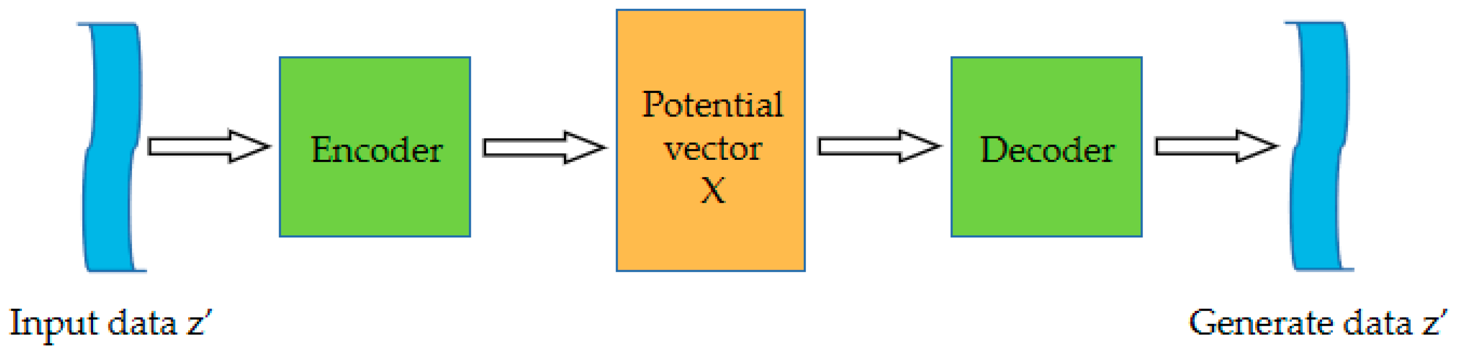
VAE is a deep generative model and a powerful learning method applied to fields such as images and language. It is an extension of the auto-encoder and has the same structure as the auto-encoder, consisting of an encoder, a latent space, and a decoder. In addition to these structures, VAE also adds a sampling layer that allows the model to generate new data from the latent space. The structure of the VAE model is shown in Figure 1.

Figure 1.
Variational auto-encoder structure.
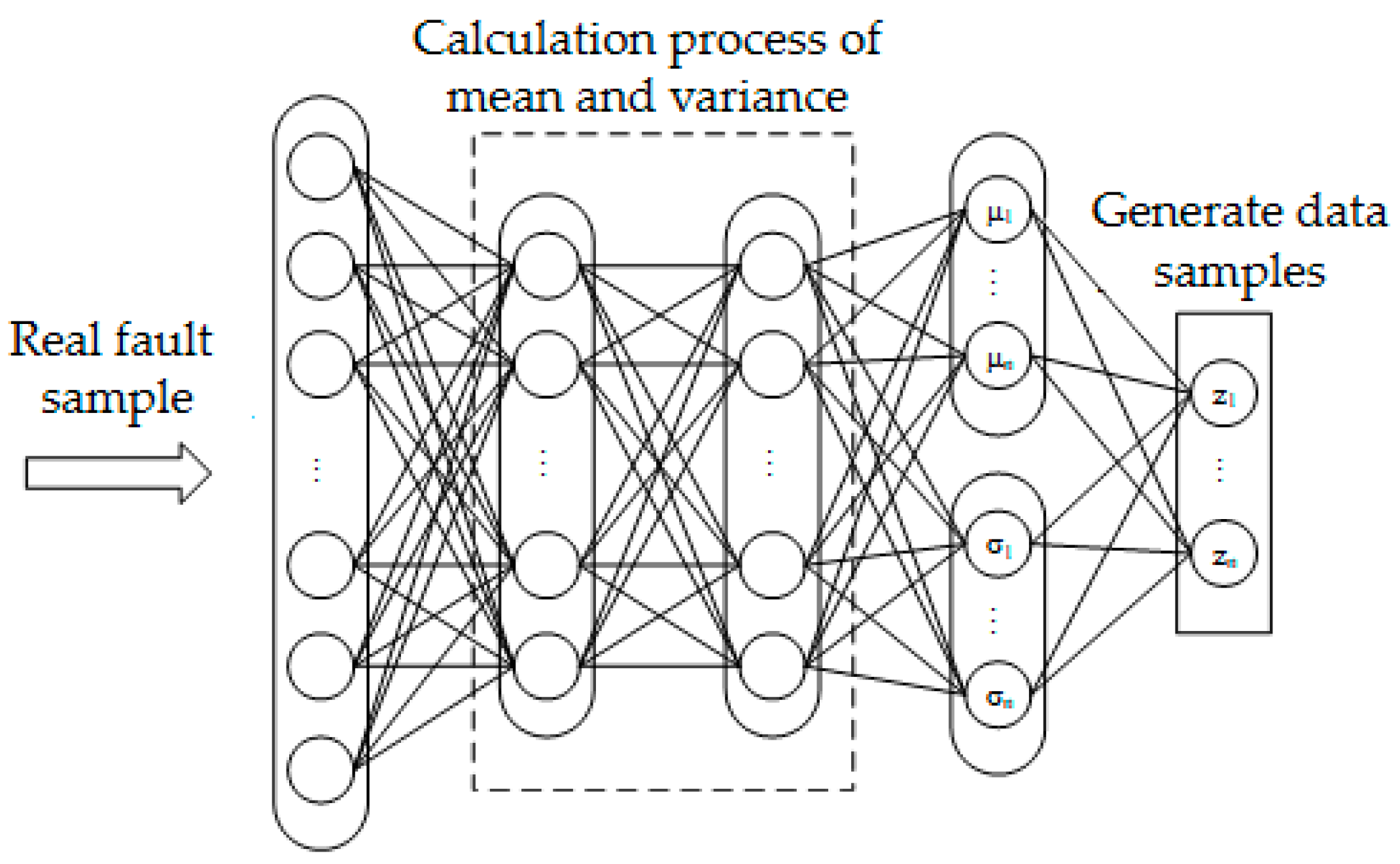
The variational self-coding network constructs the encoder based on the effective loss standard, so that the extracted features obtain a good topology similar to the input data, and the encoded output features are used as the synthesis standard of the decoder, identify the differences between the output and input data according to the appropriate objective function, and shorten the distance between the targets by modifying the weight and bias parameters. The probability distribution of the real fault set obtains the potential expression of the input samples, including mean and variance, through KL divergence learning distribution and coding calculation, so that the generated samples are similar to the real fault samples. The variational self-coding network model is shown in Figure 2.
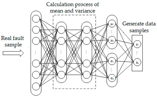
Figure 2.
Variational auto-encoder network model.
VAE can learn the distribution of data through the encoding process, which is equivalent to mastering the noise distribution corresponding to various data. Therefore, using VAE for data preprocessing can generate the required data through the specific noise obtained by learning. Since it directly calculates the mean square error between the generated data and the original data, without adversarial learning, the use of VAE may make the generated data unrealistic.
2.2. Improved Generative Adversarial Network
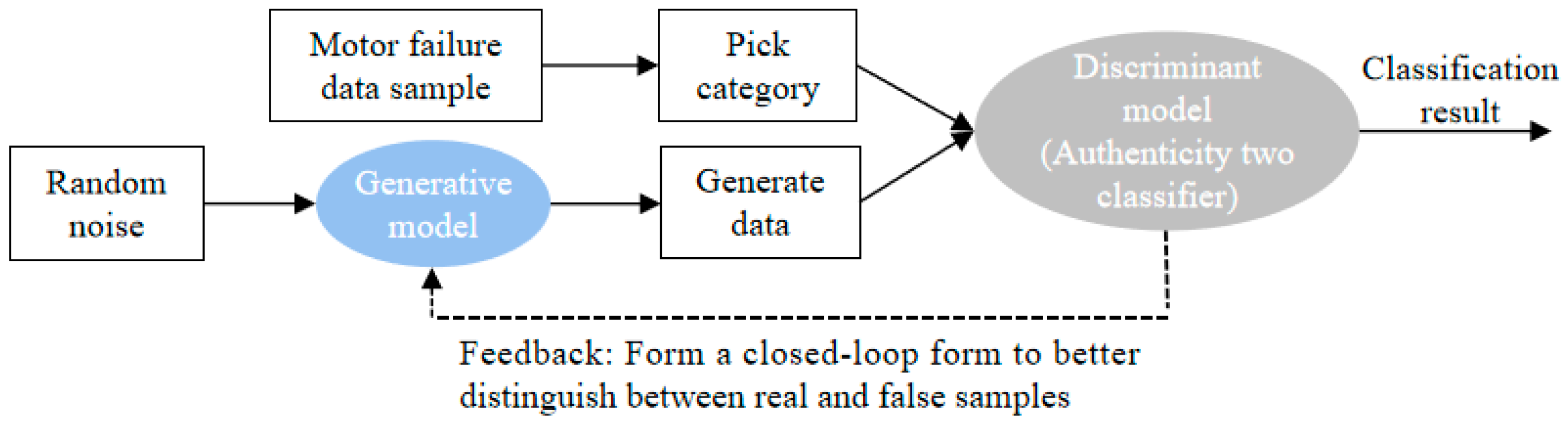
GAN is an unsupervised probability distribution learning method. Conventional GAN consists of two parts, namely the generator (G) and the discriminator (D), which train and game with each other. GAN mainly adopts the idea of mutual confrontation to improve the quality of the generated data. Random noise z is used as the input training generator to generate fake numbers, so that the discriminator will not recognize them as generated samples. The discriminator takes the real training data and the pseudo samples generated by the generator as input for training to distinguish the generated samples from the real data. The training model of GAN is shown in Figure 3.
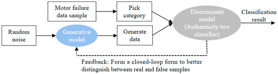
Figure 3.
GAN training model.
In general, the JS divergence is usually used to measure the probability distribution distance of the classic GAN model, but when there is no intersection between the real distribution and the generated distribution, the JS divergence cannot obtain stable return gradient information and is difficult to train. An effective method to solve the problem of instability in the training of the adversarial generative network is Wasserstein-GAN (WGAN), that is, training is performed by replacing the JS divergence with the Wasserstein distance.
The Wasserstein distance is used to measure the similarity between two probability distributions, which alleviates the problem of gradient disappearance during GAN training. The loss function value of the WGAN model provides a quantitative standard for the quality of the generated data, and a smaller loss value means that the generated data is more realistic. In addition, when training WGAN, instead of directly balancing the training process of the generator network and the discriminator network, the discriminator network is first optimized until convergence, and then the generator network is updated to make the whole network converge faster.
WGAN is a generative adversarial network that optimizes training by using Wasserstein distance instead of JS divergence. For the real distribution and the model distribution, their Wasserstein distance [16] is:
where is the set of all possible joint distributions with marginal distributions and , when the two distributions do not overlap or overlap very little, and the JS divergence is log2. It does not change with the distance between the two distributions. The Wasserstein distance can still measure the distance between two non-overlapping distributions.
The objective function of WGAN [16] is:
Because is an unsaturated function, the gradient of the generated network parameter will not disappear, which theoretically solves the problem of unstable training of the original GAN. Additionally, the objective function of the generated network in WGAN is no longer the ratio of the two distributions, which alleviates the problem of model collapse to a certain extent, making the generated samples have diversity. Compared with the original GAN, the last layer of the WGAN evaluation network does not use the sigmoid function, and the loss function does not take the logarithm.
3. Methods
3.1. Design of Fault Feature Extraction Scheme Using DATA Expansion Method
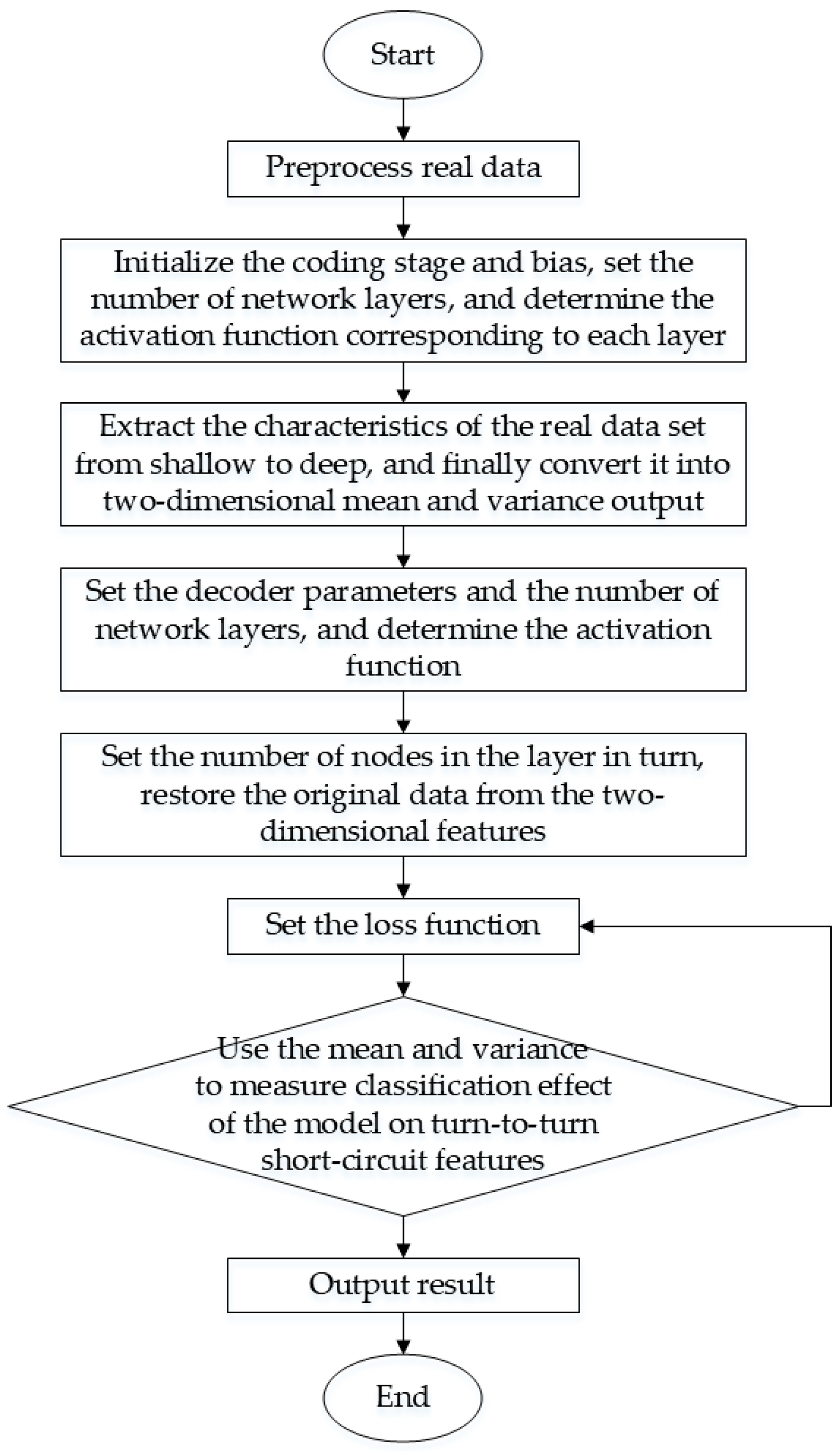
The classification model and the expansion model are combined to form a fault diagnosis model with expanded classification effects. Under different iteration times, the mean and variance of the four data sets are compared and expressed in the same coordinate system. By observing and analyzing the convergence effect of the same data set and the classification effect of different data sets, the effectiveness of the WGAN expansion method and the classification effect of VAE are verified. Figure 4 shows the feature classification scheme of turn-to-turn short-circuit fault of PMSM based on the data expansion method. The fault diagnosis steps of turn-to-turn short-circuit of permanent magnet synchronous motor are as follows:
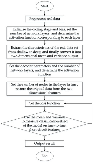
Figure 4.
Fault feature classification scheme.
- Preprocess the real data to avoid data missing and data imbalance caused by human factors.
- Set the coding model, set the number of network layers and the function of each layer.
- Set the generation/decoding model, set the number of network layers, and determine the convolution kernel of the convolutional neural network.
- Set the discriminant model, set the number of network layers, and select the optimal discriminant function as the classifier.
- Input motor fault data and extract real motor data characteristics: mean and variance.
- Restore the original data from the mean and variance to ensure that the output data has the same dimensions as the original data.
- Use two eigenvalues of mean and variance to measure the classification effect of the improved model, conduct a two-dimensional visualization analysis of the mean, quantify the classification effect, and use accuracy for comparison.
- The generated data and the original data of the improved model after training constitute the final data set of turn-to-turn short circuit fault of PMSM.
- The expanded data set is analyzed again for dimensionality reduction, and the data distribution at this time is compared with the real sample data distribution to verify the effectiveness of the expansion.
3.2. VAE-WGAN Model Structure
For motor fault data, the default value is measured by elements such as square error. Element-based metrics are simple, but they are not suitable for motor data because they cannot model the properties of human visual perception. Therefore, we advocate for the use of higher level and sufficiently constant model representations to measure data similarity. The study found that the purpose of measuring the similarity of samples is achieved through joint training of VAE and GAN. By making the VAE decoder and the GAN generator share parameters and train together, they are combined into one model. More importantly, we use Wasserstein distance instead of JS divergence to solve the problem of gradient disappearance. For the VAE training target, we replace the typical element reconstruction index with the characteristic index expressed in the discriminator.
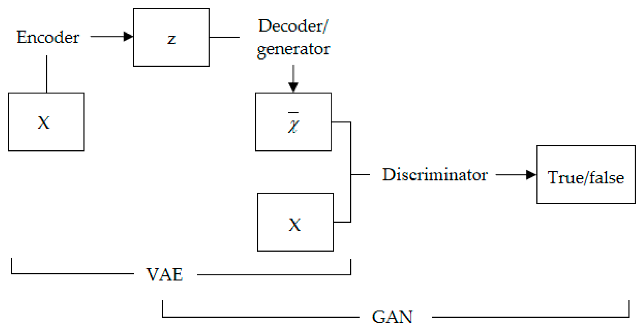
As shown in Figure 5, the overall framework of the VAE-WGAN model consists of three parts: coding network, decoding/generating network, and discriminating network. The specific function of the decoding/generation network is to restore hidden variables to noise-free data. In the training process, the discriminating network is fixed first, and the decoding network is trained to make the decoded data distribution as close as possible to the original sample distribution. Finally, the probability that the discrimination network can distinguish the decoded data as real data is 1.
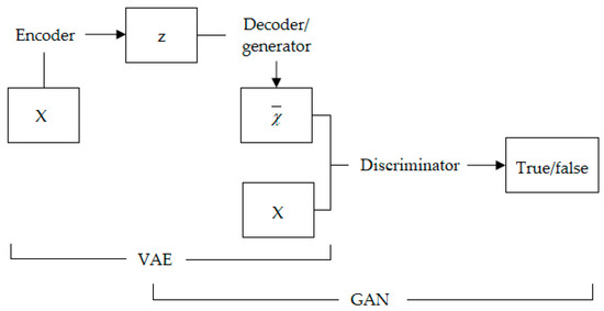
Figure 5.
VAE-WGAN model framework.
VAE-WGAN combines the two together and shares the decoder/generator to realize data generation. In the training of this structure, the discriminator provides the restriction of the true and false data, so that the reconstruction of the VAE can produce more real data. As shown in Figure 6, the z obtained in the VAE makes the input of the generator not only a completely random vector, but also encoded by real data, which is equivalent to an additional piece of supervision information (originally, the real data generated cannot be seen, so it can only learn to generate data through the output of the discriminator, and the output of the discriminator is only a scalar, which is very difficult to guide the generation of high-dimensional vectors). The final model combines the advantages of GAN as a high-quality generative model and the advantages of VAE as a method to generate the data encoder into the latent space z. Therefore, VAE-WGAN uses VAE as the generator of WGAN. Such a network not only has the characteristics of controllable data generation of VAE but also has the excellent data generation performance of WGAN.

Figure 6.
VAE-WGAN network model.
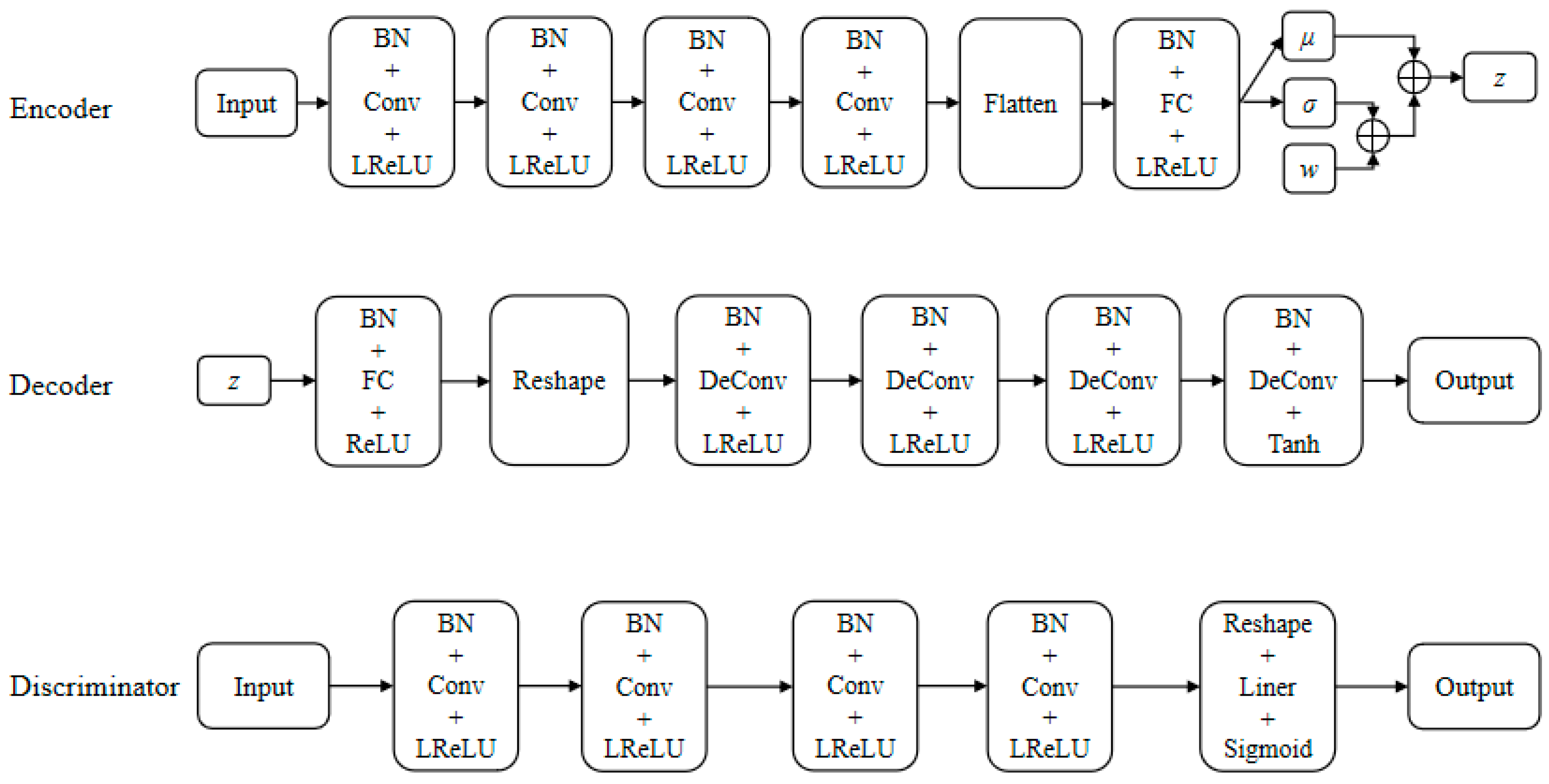
Figure 7 illustrates the detailed architecture of the encoder, decoder, and discriminator of the VAE-WGAN model proposed in this paper. The encoder, decoder, and discriminator share the same architecture. For the training experiment in this section, the model uses a convolution structure, the convolution kernel size is 3, and the post-convolution with a stride of 2 is used to amplify the data of the discriminator. The filling functions are all SAME to ensure that the data size dimensions are consistent, and the data is normalized before the activation function is activated. Post-convolution is realized by turning the direction of convolution. The model is trained using RMSProp with a learning rate of 0.0003 and a step size of 64.
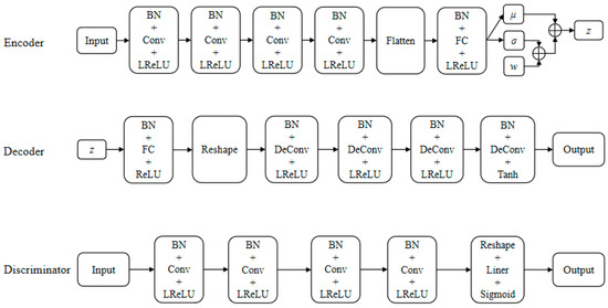
Figure 7.
Detailed architectures of the encoder, the decoder, and the discriminator of the new VAE-WGAN model.
The encoder uses four layers of convolutional layers to balance the number of extracted data features and the complexity of the network structure. The flattening layer is used to convert the multi-dimensional data generated by the convolution layer into one-dimensional data used by the full connection layer. The full connection layer is used to output the mean and variance of the posterior distribution of hidden variables. In addition to the flattening layer, all coding networks use LeakyReLU function as the activation function and all perform batch normalization (BN). These can make the network output of each layer sparser, increase the non-linearity of the whole network, prevent gradient explosion or gradient disappearance, and accelerate the convergence speed of the network. As shown in Figure 6, the coding network of VAE-WGAN consists of six layers, and the first four layers have 16, 32, 64, and 128 convolution kernels, respectively. All convolutions use the LeakyReLU activation function to transfer the flattened data to the latent space.
The decoding network consists of six layers. The first layer is the full connection layer, including 2048 neurons; the second layer is the remodeling layer, which first reshapes the one-dimensional feature vector output by full connection to 2 × 2 × 512, then the feature map is normalized in batches, and finally the normalized results are transformed non-linearly by ReLU activation function; the third to sixth layers are deconvolutional layers, with 256, 128, 64, and 32 convolution kernels, respectively. The activation function of the first five convolution layers is ReLU, and the last convolution layer uses Tanh activation function.
The discriminating network has five layers in total. The first four layers are convolution layers, with 32, 64, 128, and 256 convolution kernels, respectively, and the activation functions are LeakyReLU; the last layer is the reshaping layer, which first reshapes the input multi-dimensional data into one-dimensional data, then linearly maps the reshaped results, and finally activates the linear mapping results with Sigmoid function to output the probability of judging whether the network input data is real data. The discriminating network is a two-classifier of true and false, the structure is relatively simple, and the output probability represents the authenticity of the data.
4. Experimental Analyses
4.1. Motor Fault Parameter Acquisition
The performance parameters of the automotive PMSM used in this paper are as follows: rated power of 12 kW, rated speed of 1500 r/min, number of motor poles of 10, number of stator slots of 45, and cooling mode of water cooling. Since a rich and diverse data set can improve the learning ability of a deep neural network and avoid the over-fitting phenomenon, this paper adopted a combination of features to combine the irrelevant feature terms A-phase current, B-phase current, electromagnetic torque, and negative sequence current into a four-dimensional fault sample set.
In this experiment, 5000 groups of real motor fault samples were divided into a training set and test set in a ratio of 3:1. In total, 100 groups were sampled in each batch, with 2000 and 5000 iterations. As the number of iterations increased, the effectiveness of the model was analyzed from the following three aspects:
- The feature learning ability of VAE network changes.
- Time domain correlation analysis of generated data.
- Validity analysis of samples generated after data expansion.
This paper studies the influence of changing the number of iterations on the feature learning ability of an encoder. The dimension of the training set is reduced through the encoder to extract the final required two-dimensional hidden layer features (the features include mean and variance, and the two-dimensional mean is used as the standard in the experiment) to show the good sample reconstruction characteristics of hidden variables. The experimental analysis of the distribution of the encoder data features mapped to the two-dimensional potential space was conducted after dimension reduction.
4.2. Effectiveness Analysis of VAE Classification
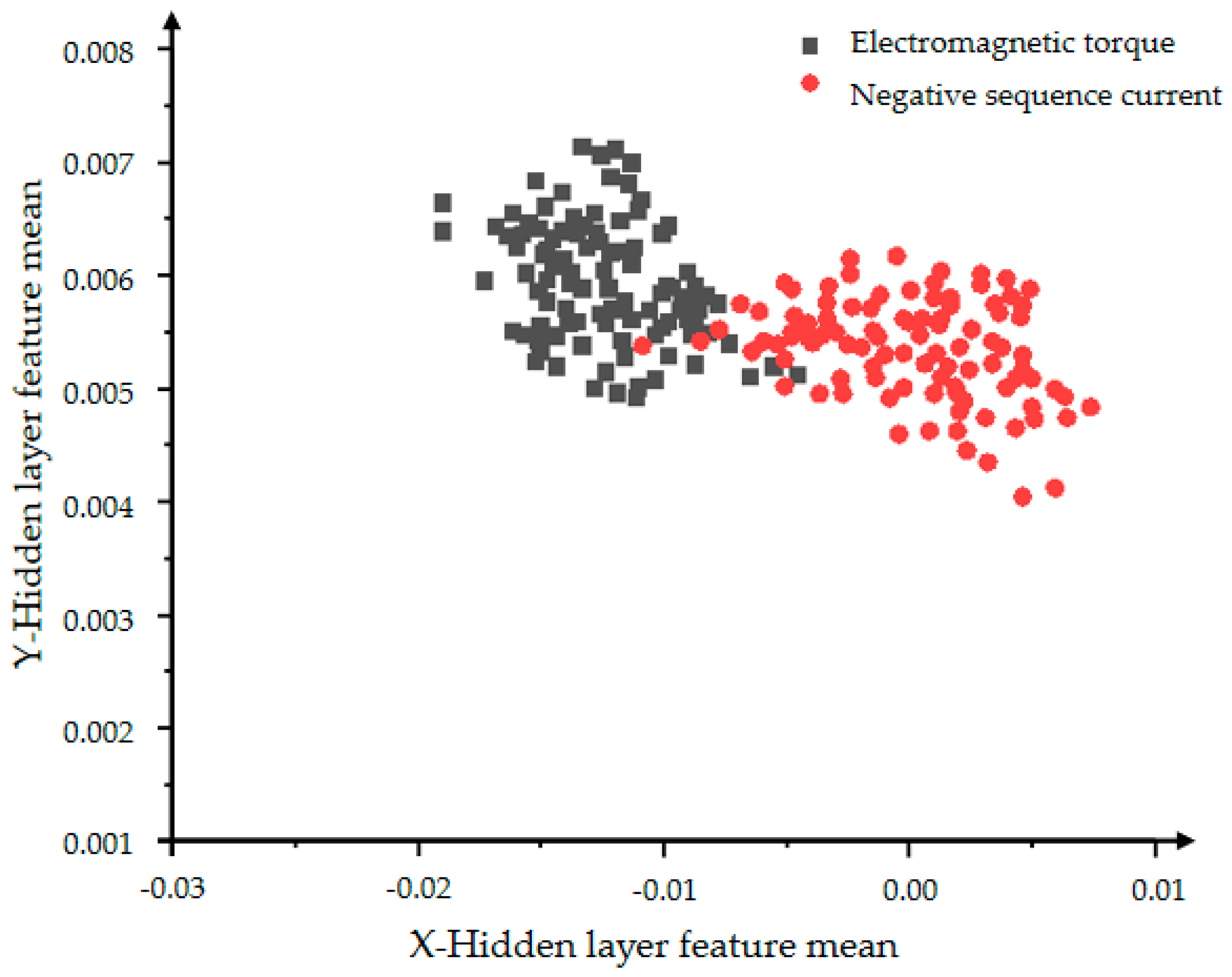
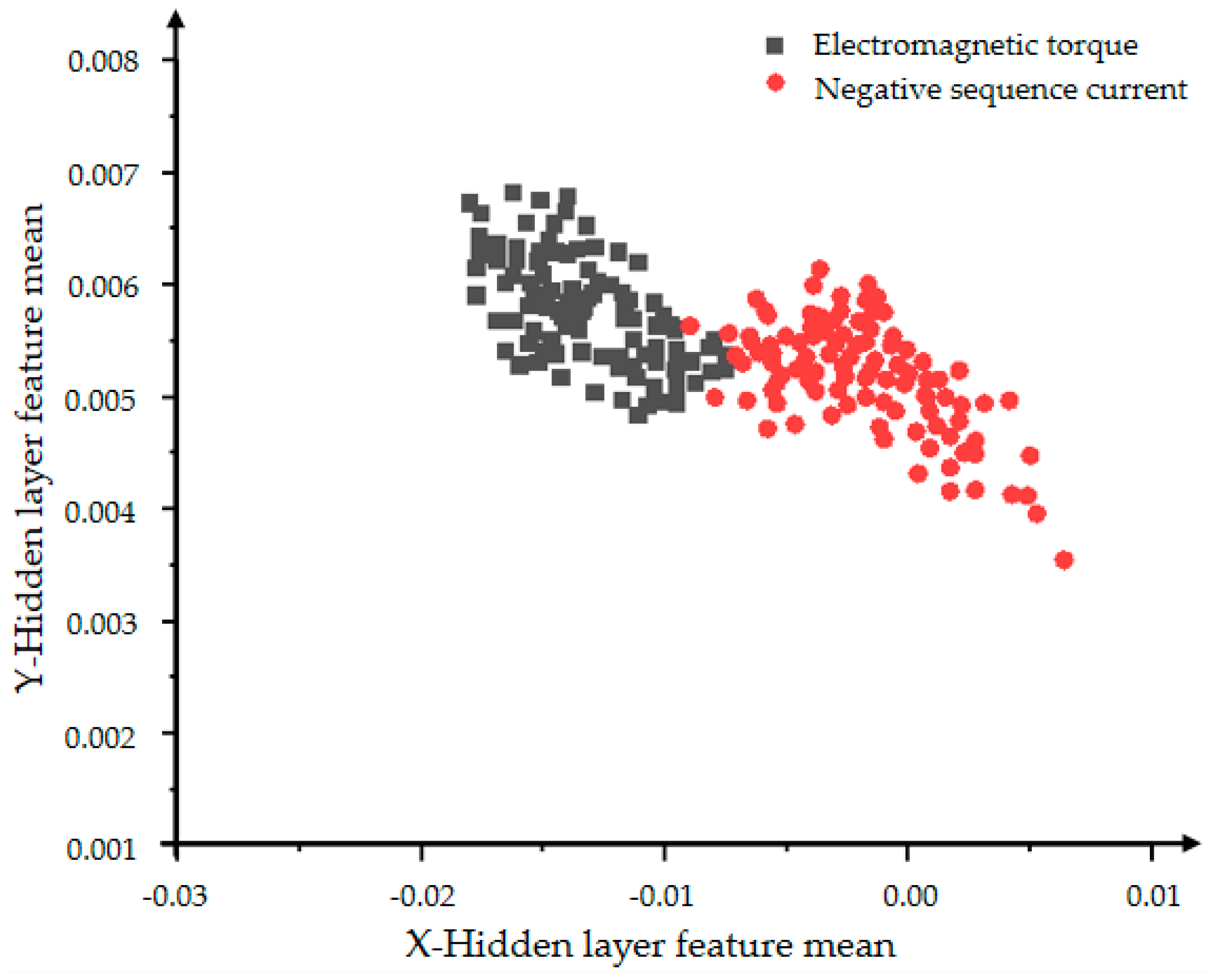
Figure 8 below shows the distribution of the mean of the extracted VAE model expanded collection data set (including expanded data and original data) in the same coordinate system. The four figures show the effect of data expansion and simple classification iterations only using the VAE model on the feature learning ability of the variational autoencoding network encoder. The dimensionality of the training set is reduced by the encoder, and the final required two-dimensional hidden layer features are extracted, and the features include the mean and the variance. The red dots in Figure 8 and Figure 9 represent the mean of the hidden layer characteristics of the negative sequence current in the state of inter-turn short circuit, and the black dots represent the mean of the hidden layer characteristics of the electromagnetic torque in the state of inter-turn short circuit. When the VAE model is iterated 2000 times, the data has no obvious signs of convergence, there is no obvious concentration area and trend, and the classification effect is poor. The model with 5000 iterations is shown in Figure 9. Compared with the data in Figure 8, it has better convergence and classification effects, and has a more obvious characteristic boundary.
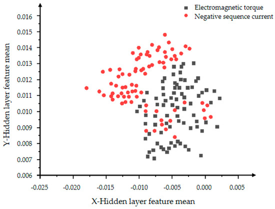
Figure 8.
The distribution of the hidden layer feature mean of the VAE model with 2000 iterations.

Figure 9.
The distribution of the hidden layer feature mean of the VAE model with 5000 iterations.
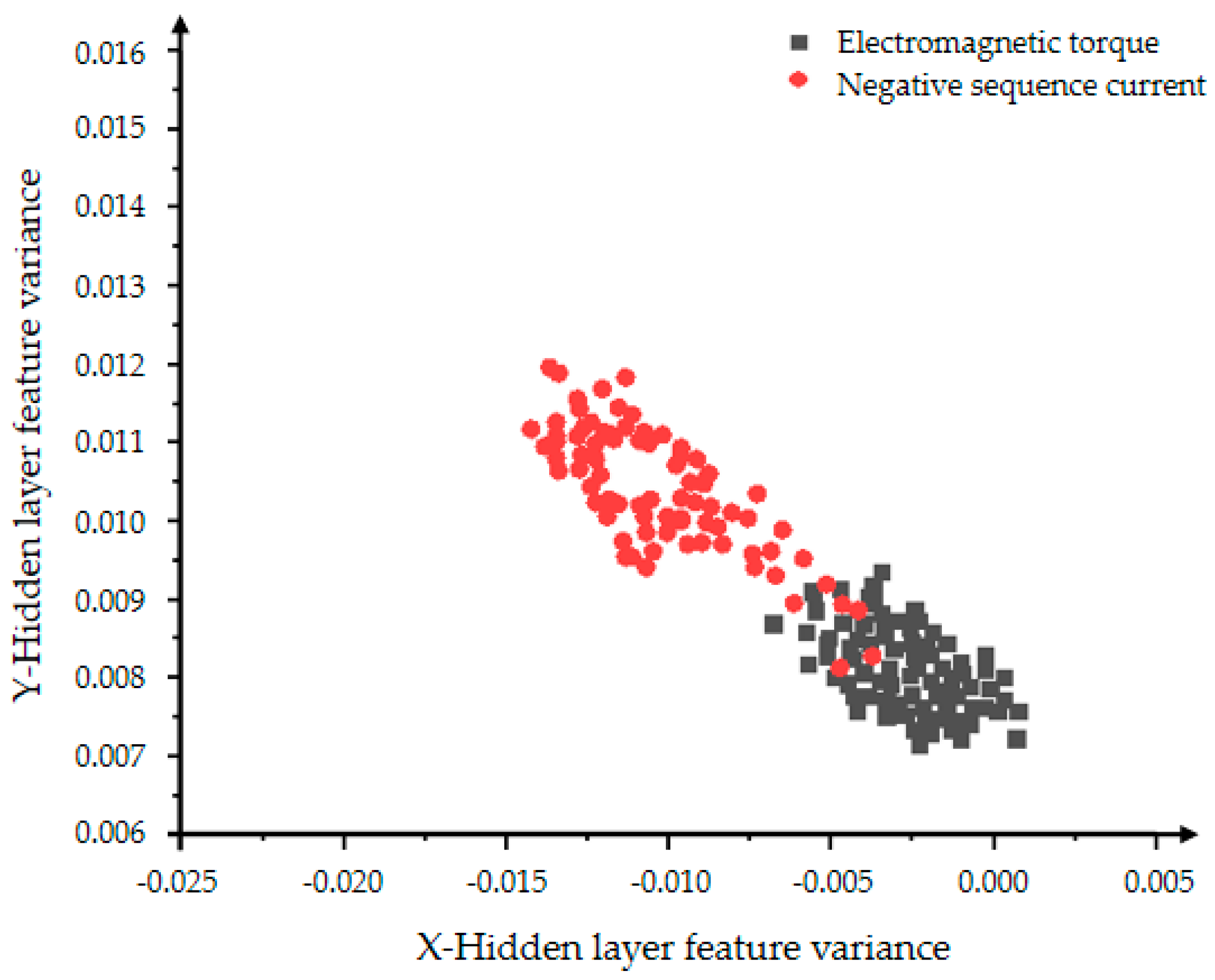
In Figure 10 and Figure 11, the red dots represent the hidden layer characteristic variance of the negative sequence current in the inter-turn short circuit state, and the black dots represent the hidden layer characteristic variance of the electromagnetic torque in the inter-turn short circuit state. Figure 10 shows a very obvious classification effect, but the data is less centralized and the features are more scattered. As the number of iterations in Figure 11 increases, the aggregation and convergence of the data are also improved to a certain extent, and the classification effect is also obvious.
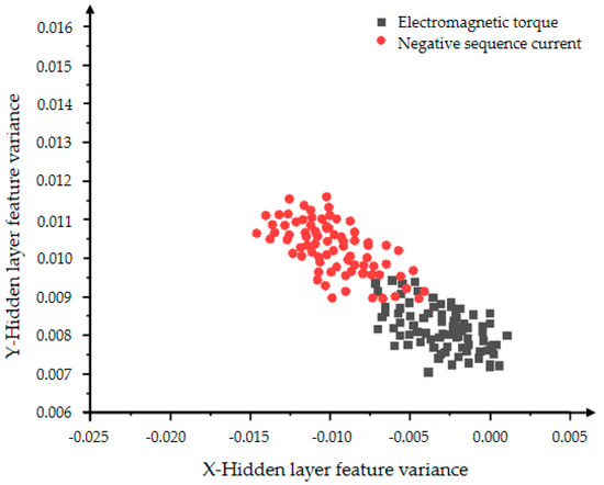
Figure 10.
The distribution of the hidden layer feature variance of the VAE model with 2000 iterations.
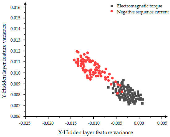
Figure 11.
The distribution of the hidden layer feature variance of the VAE model with 5000 iterations.
The comparison of Figure 8, Figure 9, Figure 10 and Figure 11 shows that the distribution rules of the two features are consistent. The experiment used the two features of mean and variance to characterize the data expansion ability and classification ability of VAE. The variational auto-encoding network was iterated 2000 and 5000 times, respectively. The comparison between Figure 9 and Figure 11 shows that the greater the number of iterations, the more mature the VAE model training is, and the better the data expansion and classification capabilities are. Experiments show that the VAE model has a strong feature classification ability, but the data expansion ability is unstable and the effect is not obvious.
4.3. Time Domain Correlation Analysis of Generated Data
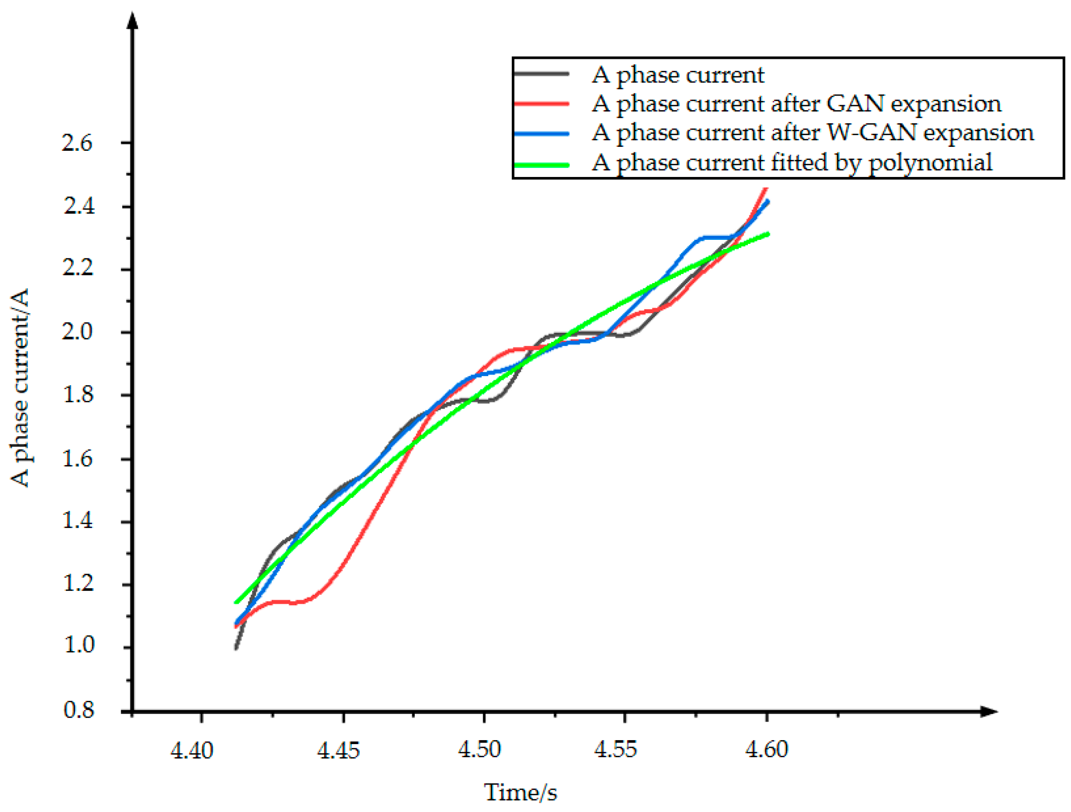
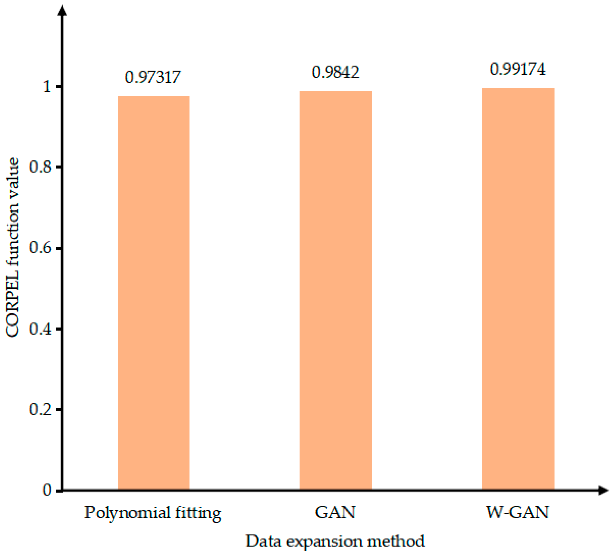
As shown in Figure 12, the time domain diagram of A phase current fault data and real fault data was enhanced by three methods in the same coordinate system. There is a large deviation near 4.45 s of the data expanded by GAN. The data generated by polynomial fitting method can describe the trend of the curve as a whole but lacks local data features. The data expanded by WGAN can better fit the original data in terms of data trend and size. Figure 13 shows the CORREL function values of the three data enhancement methods, indicating the correlation between the expanded data and the original data. It can be seen from the figure that the polynomial fitting method has the lowest data correlation after expansion. The expanded data of WGAN has the highest correlation and can best express the characteristics of the original data.
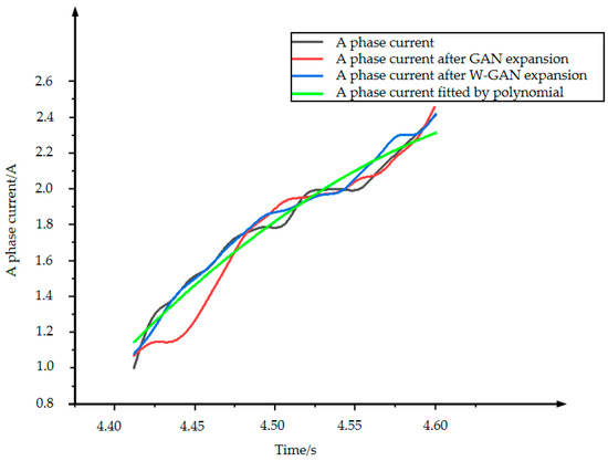
Figure 12.
A phase current expansion data comparison.
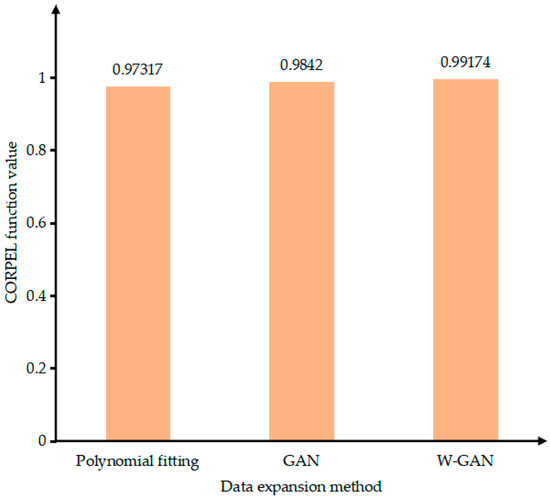
Figure 13.
Data correlation comparison of expansion methods.
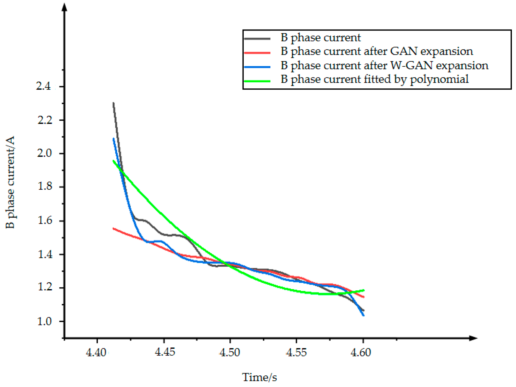
Figure 14 shows the original data and three types of expansion data of B phase current. The data expanded by GAN loses the characteristics of the original data from 4.4 to 4.48 s. Because the current tends to drop sharply near 4.42 s, the data fitted by polynomial cannot express the characteristics of the original data better, but the data expanded by WGAN can still maintain a good fit with the original data. Figure 15 shows the CORREL function values of the three expansion methods for B phase current. The WGAN fitting degree is the best, and the CORREL function value is 0.986, followed by GAN and polynomial fitting.
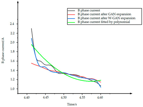
Figure 14.
B phase current expansion data comparison.
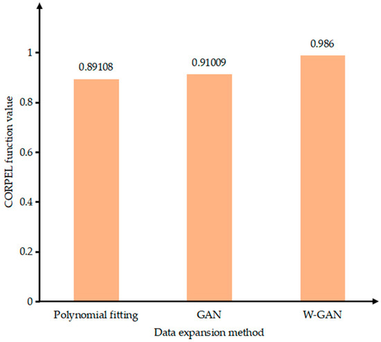
Figure 15.
Data correlation comparison of expansion methods.
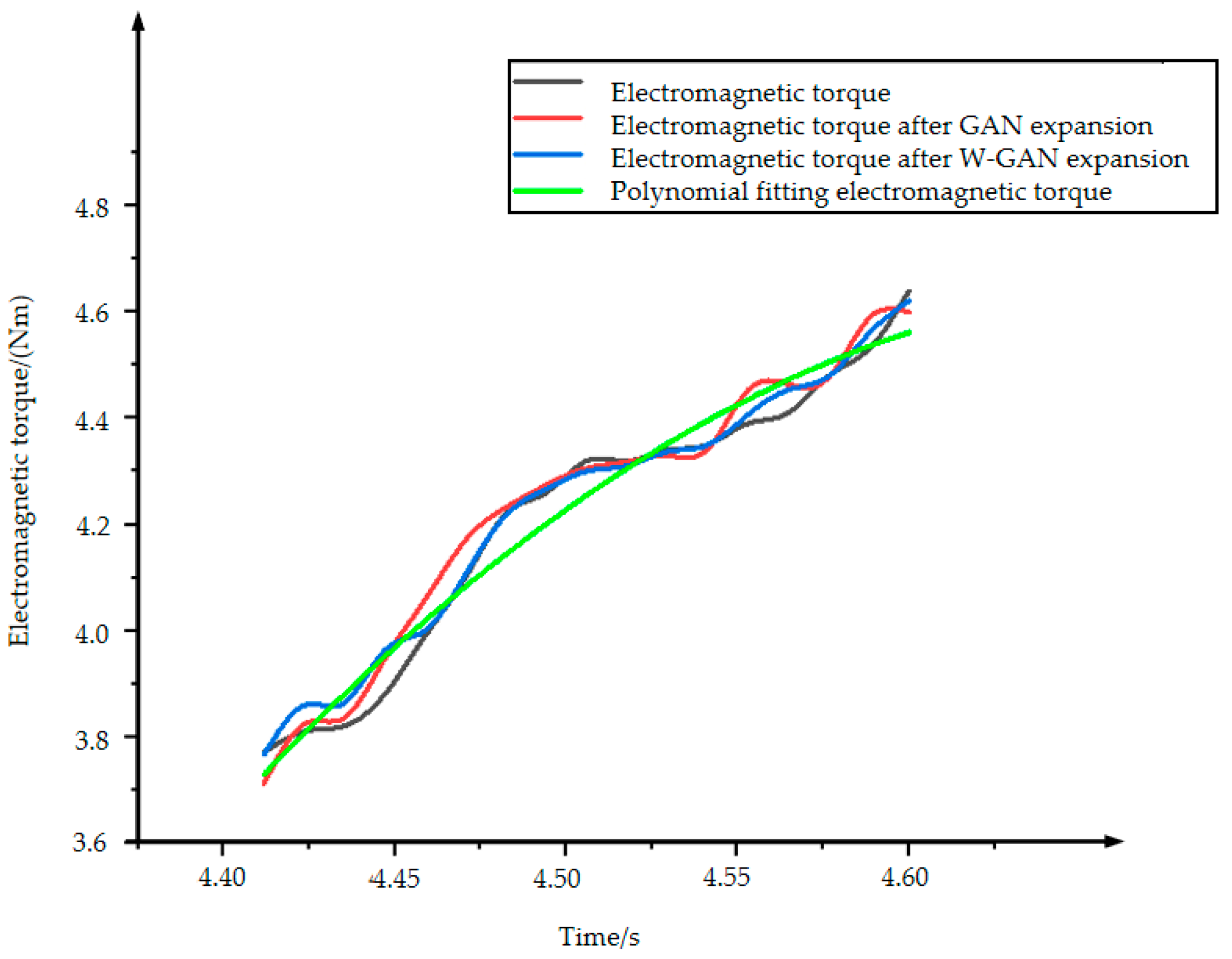
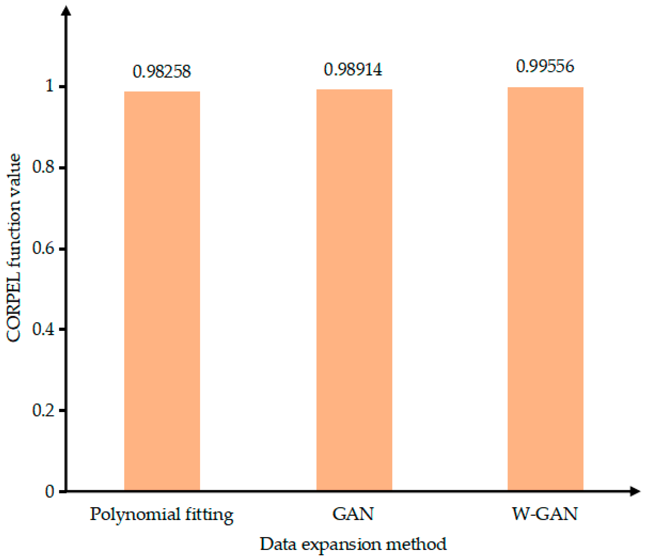
Figure 16 shows the original data of electromagnetic torque and the three types of expansion data. The data expanded by GAN has a data jump after 4.55 s, which deviates from the original data. The data using polynomial fitting has a large amount of data around 4.5 s which cannot fit the original data well. The data generated by the WGAN expansion method has a good fit with the original data as a whole and there is no partial deviation of the data. At the same time, it can be seen from the Figure 17 that the calculated value of the CORREL function between the data generated by WGAN and the original data is 0.9956. It shows that the data generated by this method has a higher correlation with the original data.
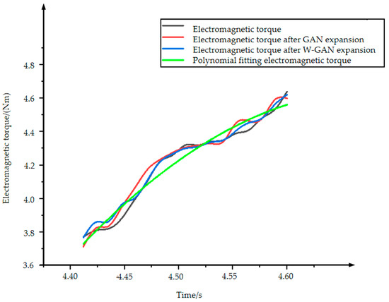
Figure 16.
Comparison of electromagnetic torque expansion data.
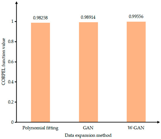
Figure 17.
Data correlation comparison of expansion methods.
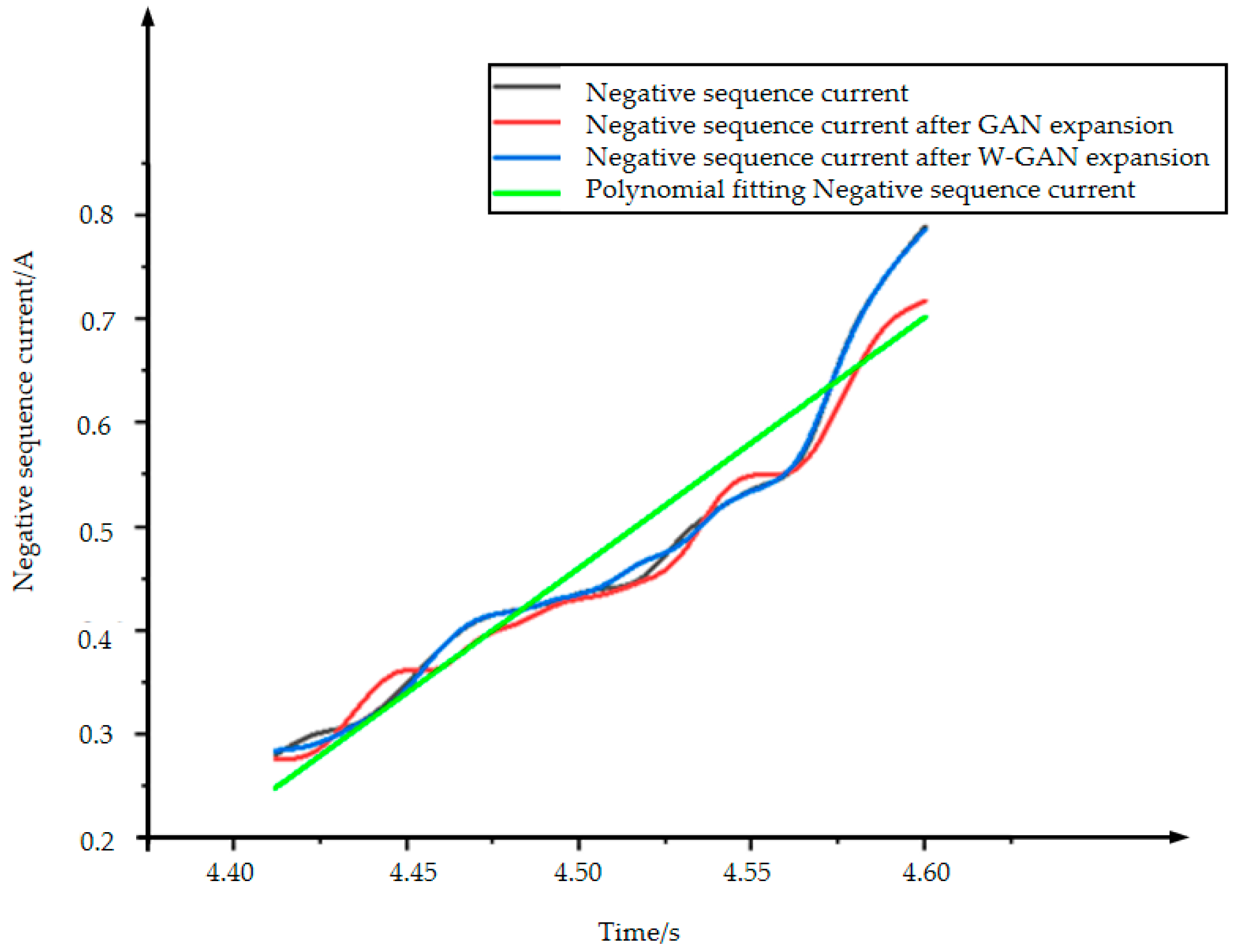
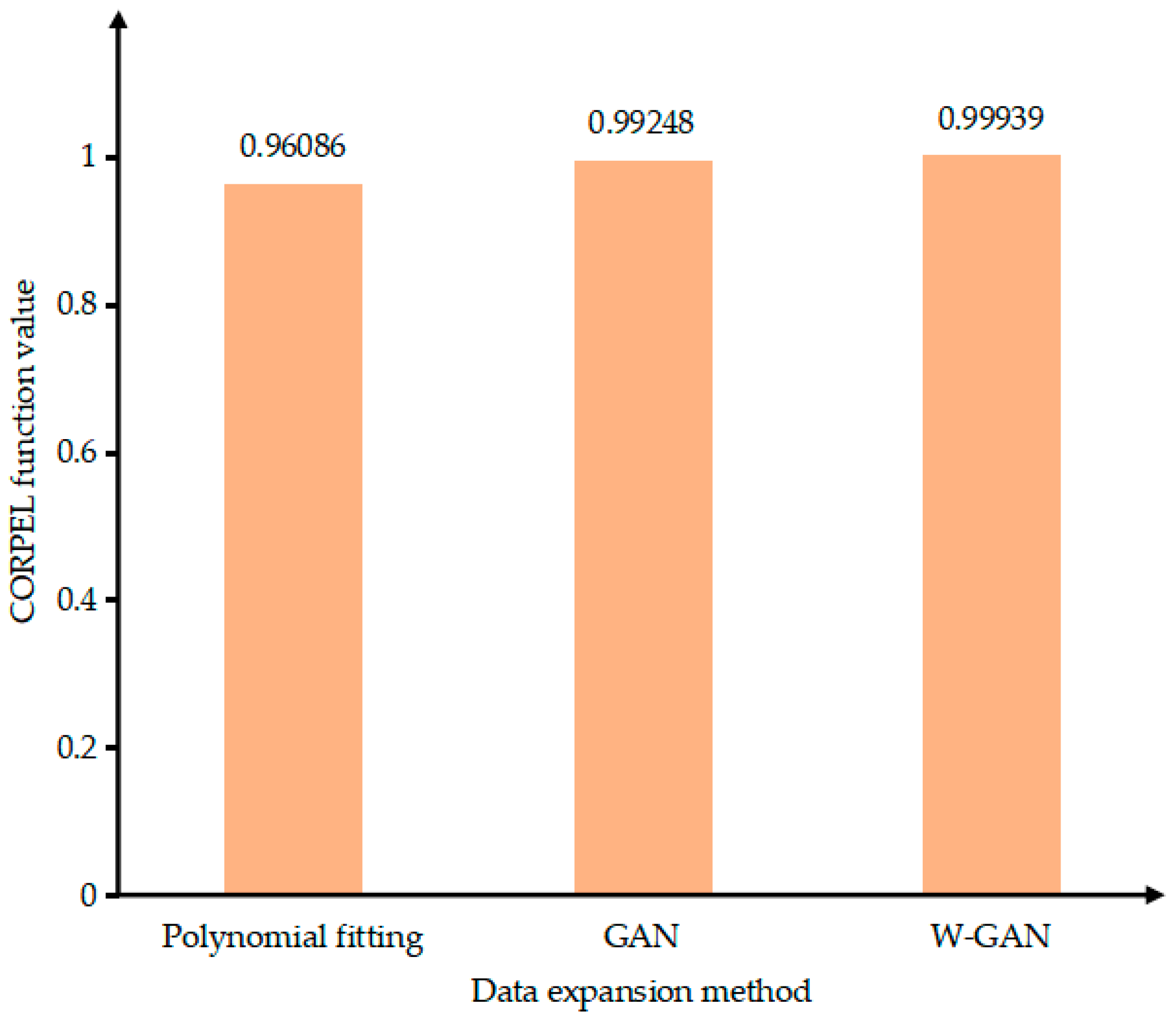
Figure 18 shows the original time domain diagram of the negative sequence current. The data after GAN expansion deviates around 4.45, 4.55, and 4.57 s, and the data is unstable. The data using polynomial fitting completely loses the original data characteristics from 4.50 to 4.57 s, and the generated data loses credibility. The data expanded using WGAN maintains a very good fit with the original data. It can be seen from Figure 19 that the CORREL function value of the data generated using the WGAN expansion method is as high as 0.99939. Therefore, compared with GAN and polynomial fitting method, the data generated by WGAN has a better fit with the original data.
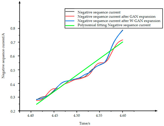
Figure 18.
Comparison of negative sequence current expansion data.
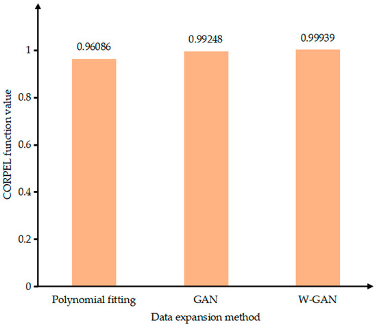
Figure 19.
Data correlation comparison of expansion methods.
Through experimental verification, the data samples generated by GAN and WGAN can meet the characteristics of real samples. However, the GAN generation model actually only learns real samples, which is one-sided and cannot represent the entire sample. GAN has a better expansion effect on core data, and the expanded data is only distributed in part of the real data. It has the advantage of concentration, but the data is not representative. The samples of WGAN not only reflect the overall advantage of change, but also the data completely contains real samples, which proves the effectiveness of WGAN model data expansion and provides an effective solution for the lack of motor fault data and imbalanced fault data.
As shown in Table 1, the data samples generated by both GAN and WGAN can conform to the characteristics of real samples through experimental verification, but the GAN generation model actually only learns real samples, which is one-sided and cannot represent the whole sample. GAN has a better expansion effect on core data, and the expanded data is only distributed in part of the real data, which has the advantage of centralization, but the data is not representative. The samples of WGAN not only reflect the overall change advantage, but also the data completely contains the real samples. It proves the effectiveness of data expansion of the WGAN model, which provides an effective solution for missing fault data and fault data imbalance of the motor.

Table 1.
Data correlation comparison.
4.4. Validity Analysis of Data Generated by VAE-WGAN
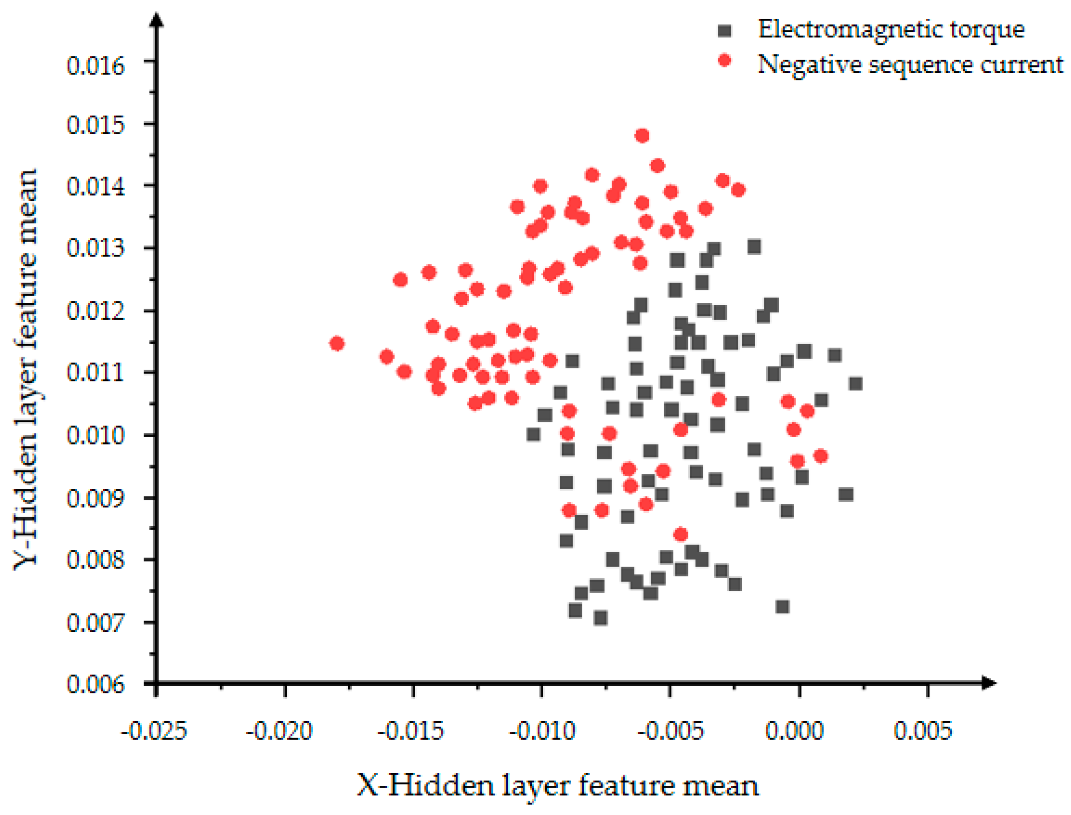
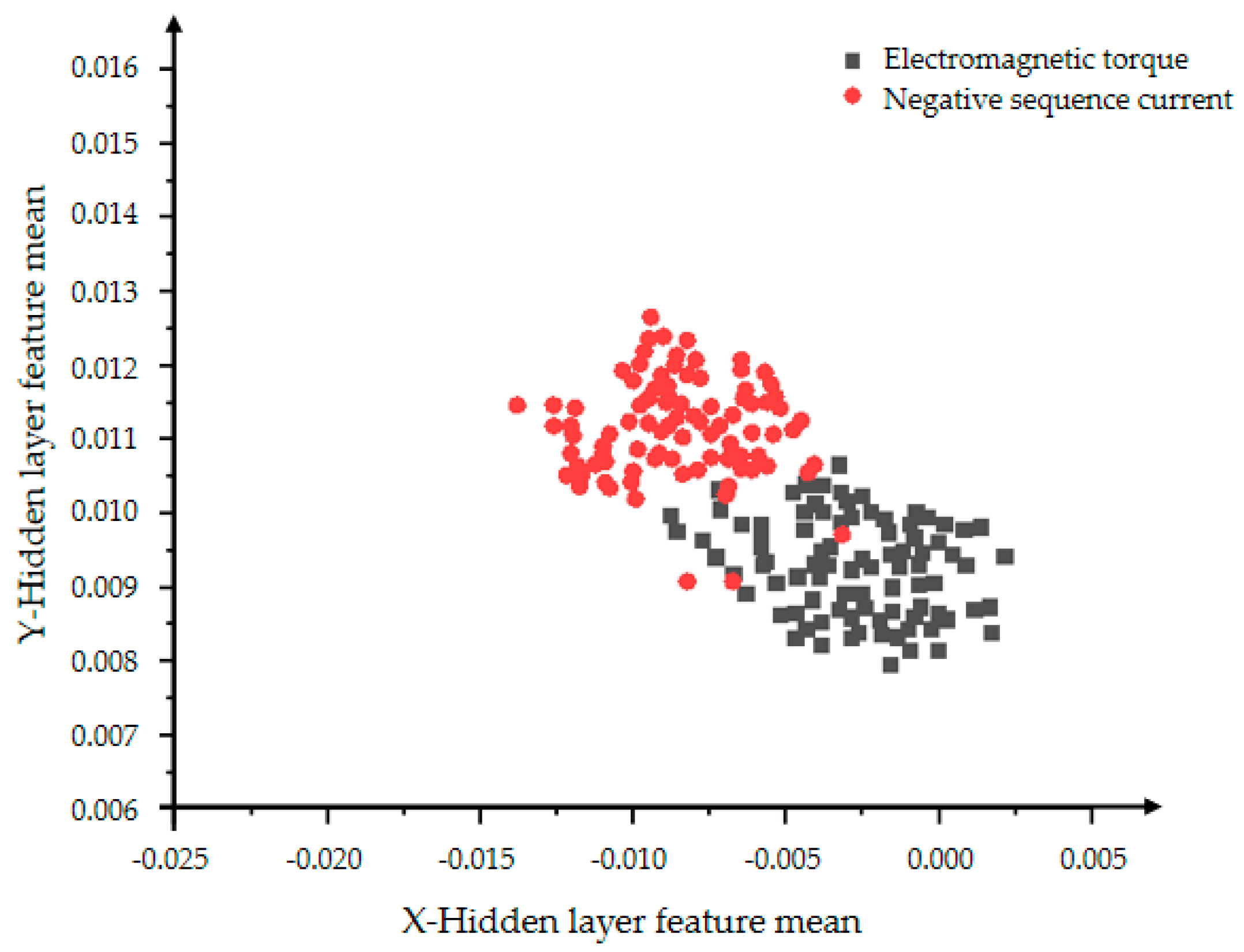
From Figure 20 and Figure 21, the influence of the number of iterations on the feature learning ability of the VAE-GAN can be obtained. The greater the number of iterations, the more obvious the feature classification. The two features of mean and variance can explain the data distribution. This section presents the feature of the mean. The black dots represent the mean of the hidden layer characteristics of the electromagnetic torque, and the red dots represent the mean of the hidden layer characteristics of the negative sequence current. First observe the distribution of individual color features. The more concentrated the distribution, the more concentrated the generated data, indicating the stronger the convergence and generation ability of the generative model. The comparison between Figure 20 and Figure 21 shows that Figure 21 can clearly divide the boundaries between different categories, proving that the classification effect of 5000 iterations is better than the effect of 2000 iterations.
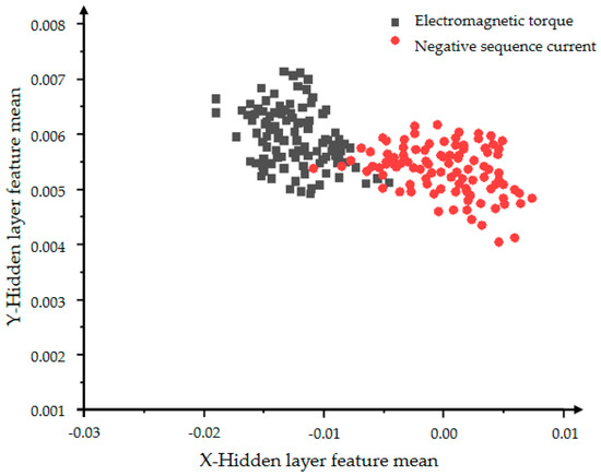
Figure 20.
The distribution of the hidden layer feature mean of the VAE-GAN model with 2000 iterations.

Figure 21.
The distribution of the hidden layer feature mean of the VAE-GAN model with 5000 iterations.
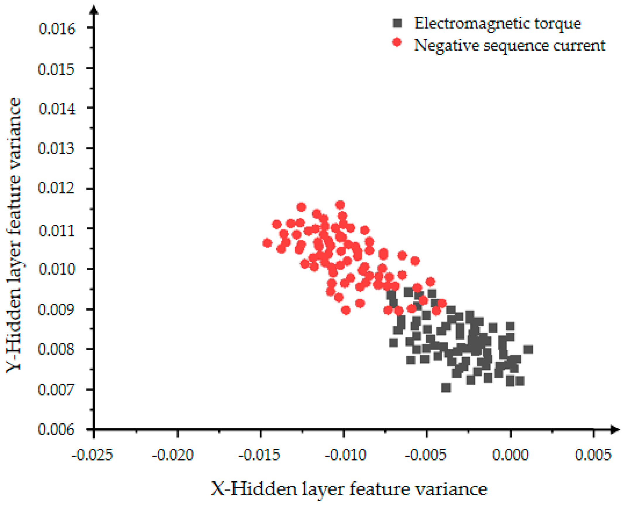
Figure 22 and Figure 23 show the hidden layer feature distributions of 2000 and 5000 iterations of the improved VAE-WGAN. Compared with the 2000 iteration effects of Figure 22, the classification effect of Figure 23 is obviously optimized. Comparing Figure 21 and Figure 23, the data generated by WGAN has better convergence, that is, the WGAN model has better convergence ability, so it can be concluded that the generation ability of WGAN is stronger than that of GAN, and at the same time it verifies the better generation ability and classification ability of the VAE-WGAN model.
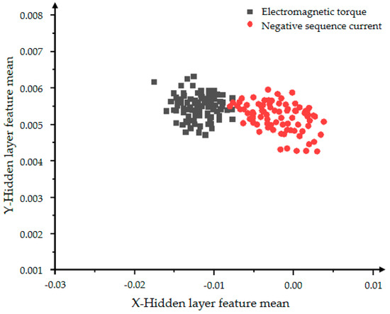
Figure 22.
The distribution of the hidden layer feature mean of the VAE-WGAN model with 2000 iterations.
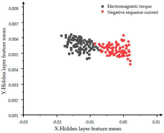
Figure 23.
The distribution of the hidden layer feature mean of the VAE-WGAN model with 5000 iterations.
4.5. Comparison of Feature Classification Models
In order to accurately obtain the model comparison results regarding the efficiency, the accuracy of sample feature classification is taken as the evaluation criterion, combined with the other three feature classification models, which are SVM-GAN, SVM-WGAN, and VAE-GAN, and compared with VAE-WGAN to analyze the optimal scheme. Accuracy is the percentage of correct results of the prediction in the total sample, that is, the ratio of the sum of the four correct classifications in this article to the total sample. The test results are shown in Table 2 below:
Table 2.
Comparison of sample feature classification accuracy of different algorithm models.
Based on the same motor sample data, the experiment iterates 2000 and 5000 times to improve the accuracy of sample feature classifications. It can be seen from the table that the feature classification ability of VAE is better than SVM, the data generation ability of WGAN is better than GAN, and the data classification accuracy of expansion after VAE-WGAN is the highest, which verifies the conclusion of Section 4.4.
5. Conclusions
In view of the characteristics of non-stationary, non-linear, multi-source heterogeneity, low value density, and imbalanced fault data collected by online monitoring equipment of permanent magnet synchronous motors, which makes the fault mechanism analysis difficult, this paper proposed a fault feature extraction method based on VAE-WGAN for a permanent magnet synchronous motor. Firstly, VAE-WGAN was selected as the fault feature extraction model and its network parameters were set. Then, the two-dimensional data features composed of mean and variance were used to fit the original data, so as to expand the data samples. Finally, these two eigenvalues were used to measure the classification effect of the improved model.
Technically, this paper combined VAE and GAN, shared the decoder and generator, and used Wasserstein distance to represent the loss function, which avoids the problem of gradient disappearance. In terms of experimental analysis, this paper used the polynomial fitting method and the comparative analysis between the original GAN and WGAN and used the CORREL function value to compare the correlation between the original data and the generated data to verify the effectiveness of WGAN expansion. The negative sequence current and electromagnetic torque were selected to extract the two-dimensional feature mean, and the visual analysis was carried out in the two-dimensional coordinate system. Through iterating 2000 and 5000 times, compared with various models, the effective classification effect of VAE, the better generation ability and classification ability of VAE-WGAN, and the highest classification accuracy were verified. The experimental results showed that the VAE-WGAN studied in this paper has good fault feature extraction effects.
Author Contributions
Conceptualization, X.X. and L.Z.; methodology, L.Z.; software, X.Q.; validation, F.Q.; formal analysis, X.X.; investigation, L.Z.; resources, X.Q.; data curation, Q.L.; writing—original draft preparation, L.Z.; writing—review and editing, Q.L., L.Z. and X.X.; supervision, X.X.; project administration, X.X. and F.Q.; funding acquisition, X.X. All authors have read and agreed to the published version of the manuscript.
Funding
This research was funded by the National Natural Science Foundation of China under Grant 51975426, the Wuhan Science and Technology Project under Grant 2019010701011393, the open fund of Hubei Key Laboratory of Mechanical Transmission and Manufacturing Engineering at Wuhan University of Science and Technology under Grant 2017A12.
Institutional Review Board Statement
Not applicable.
Informed Consent Statement
Informed consent was obtained from all subjects involved in the study.
Data Availability Statement
The data presented in this study are available on request from the corresponding author.
Acknowledgments
The authors thank all of the authors of the references cited in this article, the National Natural Science Foundation of China, and the Wuhan Science and Technology Project for supporting this work.
Conflicts of Interest
The authors declare no conflict of interest.
References
- Xu, X.W.; Qiao, X.; Zhang, N.; Feng, J.Y.; Wang, X.Q. Review of intelligent fault diagnosis for permanent magnet synchronous motors in electric vehicle. Adv. Mech. Eng. 2020, 12, 1687814020944323. [Google Scholar] [CrossRef]
- Yu, S.B.; Zhong, S.S.; Zhao, H.N.; Xia, P.P.; Guo, K. Calculation of Circumferential Modal Frequencies of Permanent Magnet Synchronous Motor. J. Harbin Inst. Technol. (New Ser.) 2019, 26, 81–91. [Google Scholar]
- Kong, Y.; Wang, T.Y.; Chu, F.L.; Feng, Z.P.; Lvan, S. Discriminative Dictionary Learning-Based Sparse Classification Framework for Data-Driven Machinery Fault Diagnosis. IEEE Sens. J. 2021, 21, 8117–8129. [Google Scholar] [CrossRef]
- Wu, G.Q.; Tao, Y.C.; Zeng, X. Data-driven transmission sensor fault diagnosis method. J. Tongji Univ. (Nat. Sci. Ed.) 2021, 49, 272–279. [Google Scholar]
- Lei, Y.G.; Jia, F.; Kong, D.T.; Lin, J.; Xing, S.B. Opportunities and Challenges of Mechanical Intelligent Fault Diagnosis under Big Data. J. Mech. Eng. 2018, 54, 94–104. [Google Scholar] [CrossRef]
- Baptista, M.; Sankararaman, S.; De, M.I.P.; Nascimento, C.; Prendinger, H.; Henriquesa, E.M.P. Forecasting fault events for predictive maintenance using data-driven techniques and ARMA modeling. Comput. Ind. Eng. 2018, 115, 41–53. [Google Scholar] [CrossRef]
- Wang, K.F.; Gou, C.; Duan, Y.J.; Lin, Y.L.; Zheng, X.H.; Wang, F.Y. Research Progress and Prospects of Generative Adversarial Network GAN. Acta Autom. Sin. 2017, 43, 321–332. [Google Scholar]
- Yao, N.M.; Guo, Q.P.; Qiao, F.C.; Chen, H.; Wang, H.A. Robust facial expression recognition based on generative confrontation network. Acta Autom. Sin. 2018, 44, 865–877. [Google Scholar]
- Goodfellow, I.J.; Pouget-Abadie, J.; Mirza, M.; Xu, B.; Warde-Farley, D.; Ozair, S.; Courville, A. Generative adversarial nets. Adv. Neural Inf. Process. Syst. 2014, 2, 2672–2680. [Google Scholar]
- Liu, Y.F.; Zhou, Y.; Liu, X.; Dong, F.; Wang, C.; Wang, Z.H. Wasserstein GAN-Based Small-Sample Augmentation for New-Generation Artificial Intelligence: A Case Study of Cancer-Staging Data in Biology. Engineering 2019, 5, 156–163. [Google Scholar] [CrossRef]
- Yong, O.L.; Jo, J.; Hwang, J. Application of deep neural network and generative adversarial network to industrial maintenance: A case study of induction motor fault detection. In Proceedings of the 2017 IEEE International Conference on Big Data (Big Data), Boston, MA, USA, 11–14 December 2017; pp. 3248–3253. [Google Scholar]
- Li, Q.; Chen, L.; Shen, C.; Yang, B.R.; Zhu, Z.K. Enhanced generative adversarial networks for fault diagnosis of rotating machinery with imbalanced data. Meas. Sci. Technol. 2019, 30, 115–120. [Google Scholar] [CrossRef]
- Wang, S.X.; Chen, H.W.; Pan, Z.X.; Wang, J.M. Reconstruction method of missing data in power system measurement using improved generative adversarial network. Proc. Chin. Soc. Electr. Eng. 2019, 39, 56–64. [Google Scholar]
- Ding, Y.; Ma, L.; Ma, J.; Wang, C.; Lu, C. A generative adversarial network-based intelligent fault diagnosis method for rotating machinery under small sample size conditions. IEEE Access 2019, 7, 149736–149749. [Google Scholar] [CrossRef]
- Shao, S.Y.; Wang, P.; Yan, R.Q. Generative adversarial networks for data augmentation in machine fault diagnosis. Comput. Ind. 2019, 106, 85–93. [Google Scholar] [CrossRef]
- Arjovsky, M.; Chintala, S.; Bottou, L. Wasserstein GAN. arXiv 2017, arXiv:1701.07875. Available online: http://arxiv.org/pdf/1701.07875 (accessed on 24 November 2021).
- Arjovsky, M.; Bottou, L. Towards Principled Methods for Training Generative Adversarial Networks. arXiv 2017, arXiv:1701.04862. Available online: https://arxiv.org/abs/1701.04862 (accessed on 24 November 2021).
- Zhang, Z.L.; Li, Y.J.; Li, M.H.; Wei, H.F. Fault diagnosis method of permanent magnet synchronous motor based on deep learning. Comput. Appl. Softw. 2019, 36, 123–129. [Google Scholar]
- An, J.; Cho, S. Variational autoencoder based anomaly detection using reconstruction probability. Spec. Lect. IE 2015, 2, 1–18. [Google Scholar]


Publisher’s Note: MDPI stays neutral with regard to jurisdictional claims in published maps and institutional affiliations. |
© 2022 by the authors. Licensee MDPI, Basel, Switzerland. This article is an open access article distributed under the terms and conditions of the Creative Commons Attribution (CC BY) license (https://creativecommons.org/licenses/by/4.0/).