Article

Detection of Bubble Defects on Tire Surface Based on Line Laser and Machine Vision

College of Mechanical and Electrical Engineering, Qingdao University of Science and Technology, Qingdao 266061, China
*
Author to whom correspondence should be addressed.
These authors contributed equally to this work.
Processes 2022, 10(2), 255; https://doi.org/10.3390/pr10020255
Submission received: 4 January 2022 / Revised: 24 January 2022 / Accepted: 25 January 2022 / Published: 27 January 2022

Abstract

:
In order to eliminate driving dangers caused by tire surface bubbles, the detection method of bubble defects on tire surfaces based on line lasers and machine vision is studied. Since it is difficult to recognize tire surfaces directly through images, line laser scanning is used to obtain tire images. The filtering method and morphology method are combined to preprocess these images. The gray centroid method is adopted to extract the center of the laser stripe, and then the algorithm to determine the positions of bubble defects on tire surfaces is proposed. According to the geometric characteristics of tire bubbles, the coordinates of starting points, ending points, and rough positions of vertices are determined. Then, the ordinates of the laser center with sub-pixel accuracy near bubble vertices are discretely magnified. The mask made of Gaussian function is convoluted with the magnified region, and the maximum value is obtained. Furthermore, the position of bubble vertices can be accurately extracted. The denoising effects of different methods for images are compared through experiments, and different positions of bubbles are detected. Experimental results show that the detection accuracy of this method is up to 93%, which is much higher than other methods. Experiments verify that the proposed method is effective for detecting tire surface bubbles.

1. Introduction

The structure of tires is complex, which can lead to the formation of bubble defects in the forming process because of the influence of material properties and the manufacturing technique. Most of the bubbles appear on the tire surface. The existence of bubbles will cause the tire to burst, which poses a great threat to driving safety and threatens the safety of people’s lives and property. Therefore, it is very necessary to detect the bubble defects in the tire-forming process, which is embodied in eliminating bubbles before tire vulcanization. Some tire manufacturers are helpless to deal with bubble defects. They usually indiscriminately use an awl to pierce the tires to be tested to eliminate bubble defects, which has low efficiency and accuracy.
At present, the most comprehensive method of automated detection of tires is by X-ray. However, considering the impact on human health, cost, and detection speed, line laser detection is superior. On the other hand, the tire surface is black. Even under the illumination of a light source, the distinction between the bubble defect and the background is not obvious, which greatly increases the difficulty of detection. Compared with the tire gray-scale value, the line laser has a higher gray-scale value. It can show the changes of the tire surface intuitively, which is helpful to the detection of bubbles.
Using curvelet transform and the Canny edge detection method, studies [1,2,3] have accurately detected foreign bodies and bubbles inside the tire by studying the texture characteristics of defects. In the aspect of tire bubble detection, the line laser is rarely used, but it is still widely used in three-dimensional scanning [4,5,6,7,8,9,10,11], obtaining distance information [12,13,14,15,16,17], surface defect detection [18,19], and production detection [20,21,22]. Lv et al. [23] used a line laser for the longitudinal detection of conveyor belts and proposed the IGGM algorithm to extract the center of the laser stripe, which can effectively remove the influence of the environment on the line laser. It is very common to use line lasers to detect welds. Zou et al. [24] proposed a weld feature point tracking algorithm based on WLCS, which can work in a strong-interference environment and has strong robustness. Additionally, line lasers are also widely used in aerospace and other advanced fields, which have high technical content. Soonkyu et al. [25] put forward the CLLST system to get the ROI image, which completes the task of detecting weld tracking points efficiently. In the process of tire bubble detection, compared with the above research, there are similarities between the acquisition of target images and the processing method of line lasers in this paper, which is worth learning.
Because of the advantages of line lasers, such as safety, simple structure, low cost, and high robustness, the line laser is used as a light source to obtain tire defect images. Because the camera is greatly affected by the light when receiving the line laser, the experiment was carried out under stable lighting conditions. In this paper, combining image filtering and morphological methods to process the image, the gray centroid method is utilized to effectively extract the center of the laser stripe. Furthermore, this paper innovatively proposes a tire surface bubble defect judgment algorithm. According to the processed laser shape, the coordinates of the starting points and ending points of the bubbles and the approximate position of the vertex are determined; then, some sub-pixel points of the vertex are magnified discretely, and the maximum value is calculated by the convolution of this part of the pixels with a special mask to accurately extract the positions of the bubbles. The main contribution of this paper is to use line lasers and machine vision to complete the detection of bubble defects; together, they can obtain the exact location of bubble defects, overcome the shortcomings of manual operation, improve detection efficiency and accuracy to a higher level, and make defect detection tend to the development of automation.

2. Image Preprocessing

In order to facilitate the subsequent processing, a unified image standard is first established, and the image format is unified with the size of 800 × 600 pixels. The image is regarded as a pixel matrix T : u ( h , l ) with a width of 800 and a height of 600, in which h represents the row of the matrix, l represents the column of the matrix, and u ( h , l ) represents the corresponding pixel value at this point.
The tire image is obtained by the laser triangulation method. The line laser transmitter is placed at a certain angle to the CCD camera. Generated by the line laser transmitter, the laser plane is perpendicular to the tangent plane of the tire slice, as shown in Figure 1. The laser plane is formed by the emission center of the line laser transmitter and the line laser. When the laser plane is parallel to the camera plane and both of them are perpendicular to the working plane, the image has only one straight laser line, which is obtained from the camera. When they are at a certain angle, it can be clearly seen that the laser line changes with the change of tire surface shape.
Due to the uneven surface of tire material, the surface roughness is high. Under the irradiation of the line laser, a large amount of diffuse reflection will be formed. After being received by the camera, a large amount of speckle noise will appear, which can cause the formation of a bright “burr” near the laser stripe. Additionally, the quality of the line laser will also be affected. It has a great degree of influence on the subsequent image processing, which needs to be effectively removed by image filtering.

2.1. Image Filtering

The purpose of image filtering is to deal with noise, which may exist in the image. Common noise processing methods include mean filtering, median filtering, and Gaussian filtering. The above three filtering methods are used for image processing, and the results are shown in Figure 2.
From Figure 2b,d, it can be seen that mean filtering and Gaussian filtering have different degrees of laser stripe blur at the position of the bubble. Compared with the original image, the median filtering has a certain ability to remove noise and retain certain edge information. Compared with Figure 2c,d, the latter is not as good as the former in the brightness of the laser stripe and the clarity of the edge. By comparing the three filtering effects, median filtering can be used as image preprocessing to achieve a better filtering effect; the median filtering is defined as
f ( i , j ) = m i d d l e { u ( h , l ) [ 1 1 1 1 1 1 1 1 1 ] } .
In Equation (1), f ( i , j ) is the pixel matrix preprocessed by median filtering, and u ( h , l ) is the pixel matrix of the original image. The median filtering convolutes u ( h , l ) with the matrix (3 × 3) whose elements are all 1, and then it sorts from large to small to take the middle value f ( i , j ) .

2.2. Morphological Processing

After filtering, the gray-scale image can be obtained. The morphological method can be used to deal with the “burr” phenomenon of the laser stripe edge and the hard impurities, which may be attached to the surface. The threshold Th of the gray-scale image obtained by the Ostu method [26] is 119. In order to retain part of the image information, the pixel gray-scale value larger than the threshold Th is reserved, which means f ( i , j ) = f ( i , j ) ; the pixel gray-scale value smaller than the threshold Th is 0, which means f ( i , j ) = 0 . The morphological processing results of the filtered image are shown in Figure 3.
From Figure 3b, it can be seen that the opening operation removes the redundant spots, which may exist in Figure 3a, and removes some edges and corners at the edge of the laser stripe to make it more rounded and smooth. As shown in Figure 3c, after expansion and corrosion, it is obvious that noise still exists, which cannot achieve the requirements of removing redundant spots.
Further trying three-dimensional gray-scale analysis for different preprocessing combinations, the results are shown in Figure 4. Compared with Figure 4a,e, the combination of Figure 4d is too natural at the junction, so median filtering and open operation are used for image preprocessing. They can ensure the clearness of the center of the laser stripe to the maximum extent.

2.3. Extraction of the Center of the Laser Stripe

Different from only operating on a gray-scale image, the core of the line laser is the extraction of the center of the laser stripe; that is, the line laser with certain pixel width is extracted into a laser center with only one pixel width so as to improve detection accuracy. At present, the Steger algorithm [27], the gray centroid method, and the improved laser extraction algorithm [4] are commonly used.
Ding X.D. combines the extreme value method with the gray centroid method to extract the center of the laser stripe, which ensures the accuracy of weld detection [28]. Since the research object is the tire after forming and before vulcanization, the gray-scale value of the image is close to 0, and the texture is relatively single. The linear dependence between each pixel is small, there are fewer patterns and characteristics, and there is a large gray-scale difference between the line laser and the tire. The Steger algorithm is not suitable for the case where the width of the laser stripe changes greatly, so the gray centroid method is used to extract the center of the laser stripe.
The gray centroid method traverses the whole-image pixels from left to right. Then, the weighted centroid coordinates of each column can be obtained; that is, the gray centroid is defined as Equation (2).
m = β 1 , ( β N * ) n = j = 1 p = 800 i = 1 q = 600 i f ( i , j ) j = 1 p = 800 i = 1 q = 600 f ( i , j )
The center of the whole laser stripe is obtained by connecting the gray centroid of each column. The center value of laser stripe calculated by the gray centroid formula is usually decimal, which has high accuracy and can reach the sub-pixel level.
As shown in Figure 5, the center of the laser stripe is extracted by the gray centroid method. The red scattered points in the figure represent the center of each column of laser stripes calculated, and the yellow broken line segments are used to connect the center points of laser stripes. The increasing or decreasing trend of the laser stripe can be seen in Figure 5. According to the trend, this paper proposes the judgment algorithm for bubble defects on the tire surface.

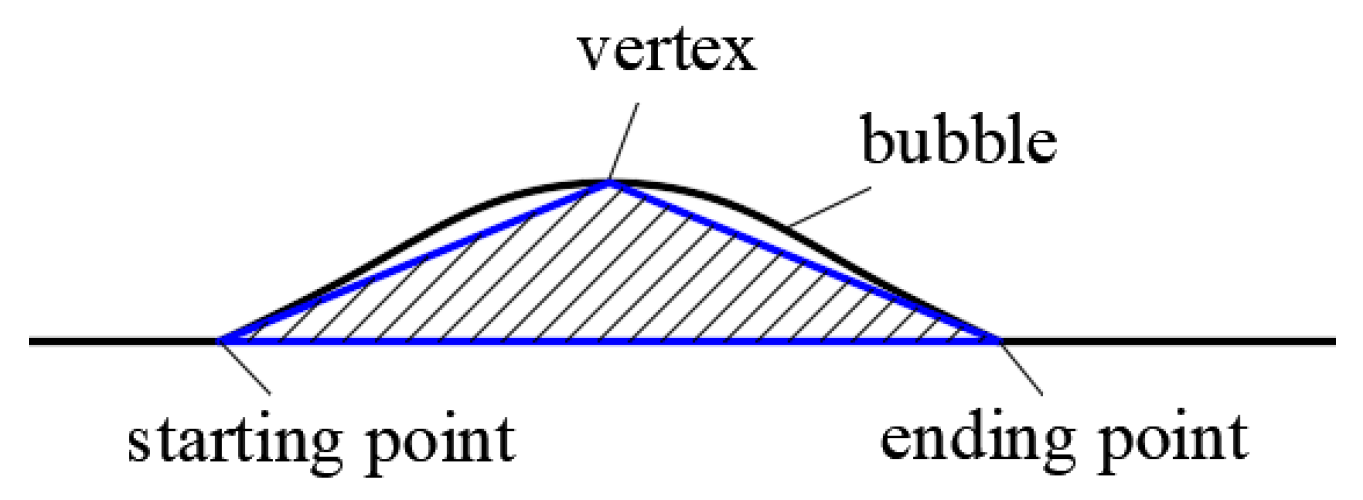
3. Bubble Defect Position Judgement

Different from traditional image detection, which needs complex algorithm processing, the line laser is more direct for defect detection. Compared with the laser stripe under normal irradiation, if the laser line is bent to a certain extent in some segments, there is a bubble defect. It can be seen from Figure 5 that the laser stripe has obvious bulges at the bubbles, and then the points where the laser stripe starts to generate bulges and end bulges can be obtained.
α ( x ) is the function represented by the center of the laser stripe of the image. In order to improve detection accuracy, to avoid the fluctuation of the points on the stripe function due to unknown factors and to reduce occasionality, it is necessary to reduce the judgment interval as much as possible. When Equation (3) is met, a set of points with the abscissa of { x 1 1 , x 1 2 , x 1 3 x 1 n } can appear, which increase in turn.
{ [ α ( x 1 ) α ( x 1 n ) ] / n < Y 1 [ α ( x 1 + n ) α ( x 1 ) ] / n > Y 1 n ( 0 , 5 )
The minimum value x 1 min of this set of data is taken as the starting point of the bubble defect. When Equation (4) is met, a set of points with the abscissa of { x 1 1 , x 1 2 , x 1 3 x 1 n } can appear, which decrease in turn.
{ [ α ( x 2 ) α ( x 2 n ) ] / n < Y 2 [ α ( x 2 + n ) α ( x 2 ) ] / n > Y 2 n ( 0 , 5 )
The maximum value x 1 max of this set of data is taken as the ending point of the bubble defect. Y 1 = 1 / 5 , Y 2 = 1 / 4 is set initially. By calculating the starting and ending points of the bubble, the position of the bubble defect can be obtained.

3.1. Single Bubble Defect

Single bubbles are a common form of tire bubble defect. After obtaining the position of the starting point and ending point of the bubble, the position coordinates of the bubble vertex should be determined. There are three types of bubble vertex positions. As shown in Figure 6, the bubble vertex is just on the middle vertical line between its starting point and ending point, and the bubble vertex is on the left or right position of the middle vertical line. Among them, Type I bubbles belong to the relatively regular and ideal type (because of the complexity of tire production, the possibility of occurrence is very small), while Type II and Type III bubbles are very common, which are steep on one side and gentle on the other.
In [29], a weighted algorithm between pixels is proposed to determine the location of defects. Therefore, a method is proposed: starting from the pixel coordinates of the bubble starting point, first move up to one pixel length and start the traversal to the right until the laser stripe is first contacted. Record the value of abscissa s 1 and the difference Δ S ( s 1 ) = | s 1 x 1 min | between the bubble starting point and the abscissa; then, continue to move up a pixel length. With the continuous upward movement, the value of the recorded abscissa s 1 and the difference Δ S ( s 1 ) will become larger and larger. When Δ S ( s 1 + 1 ) Δ S ( s 1 ) 0 , the difference of the abscissa reaches the maximum value Δ S ( s 1 ) max for the first time. At the same time, starting from the pixel coordinates of the bubble ending point, move up to one pixel length, start the traversal to the left until the laser stripe is first contacted and get the value of abscissa s 2 and the difference Δ S ( s 2 ) = | s 2 x 1 max | between the bubble ending point and the abscissa. At this time, the value of s 2 gradually decreases, and when Δ S ( s 2 1 ) Δ S ( s 2 ) 0 , the maximum value Δ S ( s 2 ) max of the difference is obtained.
It can be seen from Figure 5 that after the vertex position of the bubble defect is enlarged, there is a relatively gentle interval, which is not a peak shape in the imagination, so we have Equation (5).
x 1 max x 1 min = Δ S ( s 1 ) max + Δ S ( s 2 ) max + δ
where δ represents the length of the gentle interval at the bubble vertex when enlarged to pixel level.
When Δ S ( s 1 ) max = Δ S ( s 2 ) max , the value of δ is ignored, that is, the distance between the bubble vertex and the starting point of the bubble is the same as that between the bubble vertex and the ending point of the bubble. The bubble is located on the vertical line between the two points, so the bubble belongs to Type I. When Δ S ( s 1 ) max > ( < ) Δ S ( s 2 ) max , the top of the bubble is near to (far from) the ending point, and the bubble belongs to Type III(II). The abscissa of the bubble vertex can be given as i = s 1 + ( s 2 s 1 ) / 2 .
In order to reduce occasionality, after obtaining the pixel width of the gentle interval at the bubble vertex, all the pixels in the interval are convoluted to further improve the accuracy. In the process of obtaining the ordinate of the bubble vertex, the center of the laser stripe obtained by the gray centroid method has sub-pixel accuracy, and the value n of the ordinate has a decimal. If the ordinary pixel accuracy is used to deal with it, it will produce large errors. Therefore, rounding n to [n], the ordinates of all center points of the laser stripe in this interval can be obtained by Equations (6) and (7).
When the ordinates of the center points of the laser stripe in the interval are greater than Δ S ( s 1 ) max , it can be given as Equation (6).
j = r o u n d { ( n [ n ] ) × H + [ n ] }
Otherwise, the ordinates can be given as Equation (7).
j = r o u n d { [ n ] ( n [ n ] ) × H }
The decimal part of the ordinate is discretely magnified in proportion, and the result is rounded, which is equivalent to magnifying the sub-pixel part of the ordinates of the center points of the laser stripe and then processing. As a result, the decimal part of the sub-pixel part is removed. One dimensional Gaussian function Gauss(x) is used as the basic function, with x { 0 , 1 , 2 H } . Let σ = 1 ; the value of the corresponding Gaussian function is calculated, and the weight of each different x is obtained by normalization. As shown in Figure 7, the mask made by the Gaussian function can be given as M ( x ) = G a u s s ( x ) / x = 0 H G a u s s ( x ) .
The mask is H in length, and the mask is convoluted with all pixel points within the range of H at the bubble vertex in the order of up to down, which is equivalent to weighting and summing the part of pixel points. The center points after operation can be given as Equation (8).
U ( x = 0 ) = Σ x ( 0 , H ) f ( i , j ) M ( x )
In Equation (8), the order of i ( Δ S ( s 1 ) max , Δ S ( s 2 ) max ) is from left to right. In the traversal process, when the mask has not encountered the center points of the laser stripe, the gray-scale value f ( i , j ) of the area where the mask is located is 0, so there is U ( x = 0 ) = 0 . As the mask gradually moves down to contact the discrete magnified laser stripe points, the value of U ( x = 0 ) gradually increases until the mask reaches the center of the discrete magnified processing, which is the center position of the gentle region at the bubble vertex. Additionally, the maximum value U ( x = 0 ) max is reached; that is, the ordinate of the bubble vertex is j = U ( x = 0 ) max .
According to Equations (3), (4) and (8), the starting and the ending points and bubble vertices can be obtained, and the slope relationship between them can be calculated by Equation (9).
{ Y 1 = | U ( x = 0 ) max α ( x 1 min ) s 1 + ( s 2 s 1 ) / 2 x 1 min | Y 2 = | U ( x = 0 ) max α ( x 1 max ) s 1 + ( s 2 s 1 ) / 2 x 1 max |
By observing the bubble vertices, the starting point, and ending points of bubbles when forming a triangle, compared with the strict sense of the triangle, the bubble forms an arc instead of a straight line on its two sides. No matter how different the shape of the bubble defect is, a straight line is always included in the arc.
As shown in Figure 8, the slope corresponding to the arc line at the starting (ending) point of the bubble defect must be larger (smaller) than that of the straight line. When judging the bubble defect, if there are several groups of coordinate points in succession, the slope between them and the bubble vertex is less than (greater than) the slope between them and their respective nearby points; it is the point where the bubble starts (ends).
To sum up, the process of bubble detection is shown in Figure 9, and the specific steps are as follows:
Step 1: For the defect image with 800 × 600 pixels, the median filtering and morphological processing are carried out first, and the center of the laser stripe is extracted by the gray centroid method.
Step 2: All the pixels in the laser center are traversed from left to right, and the coordinates of the starting point and ending point of the bubble in the pixel matrix are determined according to Equations (3), (4) and (9).
Step 3: Use the starting point and ending point to get the position i ( Δ S ( s 1 ) max , Δ S ( s 2 ) max ) of the gentle interval at the bubble vertex, and all pixels in the interval are weighted and summed to obtain the maximum value, which is the coordinate value U ( x = 0 ) max of the bubble vertex.
Step 4: The starting point, ending point, and bubble vertex are obtained, and the detection of the bubble is completed.

3.2. Real-Time Processing

In the process of real-time detection, it is inevitable that the same bubble defect will be detected not only once. In order to reduce repeated judgment, improve detection efficiency, and save time, a bubble is photographed by CCD cameras many times. The root, middle, and vertex of the bubble front are detected, respectively, to confirm whether they belong to the same bubble. The principle is shown in Figure 10.
Through the extraction of the center of the laser stripe at the root, middle, and vertex of the same bubble front, it can be found that different positions of the bubbles irradiated by the line laser lead to different bulge degrees of the center of the laser stripe, but the abscissa of the arc bulge of the bubble is the same. The abscissa corresponding to the center position of the bubble can be calculated by ( x 1 min + x 1 max ) / 2 ± ε , where ε is the deviation of camera shooting caused by mechanical vibration and the error of image processing. Judging whether the former and the latter are within a reasonable range, it can detect whether the bubble defects from different pictures belong to the same bubble. Once the same bubble is detected, it will not be detected again. As the bubble moves, the line laser irradiates the side of the bubble away from the camera so that the line laser in this part is blocked by the bubble. It misses a part of the line laser from the camera angle of view. At this time, it is still judged as a bubble until the laser stripe of this part is completely exposed; that is, the laser stripe becomes a straight line again, and then the confirmation of the bubble is completed.

3.3. Multiple Bubble Defects

In the tire production line, due to the complex and unpredictable characteristics of bubble generation, there are a variety of bubble locations, and two or more bubbles may appear simultaneously on a line. It can be seen from Figure 11 that there are two arc bulges in the center of the extracted laser stripe. After traversing the image pixels, the maximum and minimum coordinate arrays of two groups of points can be obtained. From Equations (3) and (4), the starting and ending points of two bubbles can be obtained, which are x 1 min , x 1 max , x 2 min and x 2 max . From left to right, the relationship is as follows: x 1 min < x 1 max < x 2 min < x 2 max , where x 1 min and x 2 max can be obtained directly, but x 1 max and x 2 min are in the middle position, which cannot be directly obtained. The array λ can be obtained by Equation (3) with two sets of rising points. The array θ can be obtained by Equation (4) with two sets of declining points. Similar to the acquisition of a single bubble point in Section 2, x 2 min and x 2 max of the second bubble can correspond to two arrays of { x 2 1 , x 2 2 x 2 n } and { x 2 1 , x 2 2 x 2 n } . When x 1 max = x 2 min , two bubbles are adjacent to each other so they can be treated as one bubble, which does not belong to the treatment category of multiple bubbles. When x 1 max x 2 min , the value of x 1 max and x 2 min can be calculated by Equations (10) and (11).
{ x 2 min = min ( | x 1 min + x 2 max 2 λ | ) λ { x 1 1 , x 1 2 x 1 n , x 2 1 , x 2 2 x 2 n }
{ x 1 max = min ( | θ x 1 min + x 2 max 2 | ) θ { x 1 1 , x 1 2 x 1 n , x 2 1 , x 2 2 x 2 n }
Using Equations (10) and (11) to deal with arrays λ and θ , taking the middle value of x 1 min and x 2 max , then finding the absolute value of the minimum difference between the middle value and the two array, respectively, the value of x 2 min and x 1 max can be determined. Then, the starting and ending points of the two bubbles can be obtained, and their specific positions can be determined. As for more bubbles (>2) on the same laser stripe, it is less accurate. The complexity of the algorithm will be improved, so it is not considered.

4. Experimental Result

The camera used in the experiment is Hikvision, the graphics card of the computer is GTX860M, the video memory is 2 GB, and the processor model is i5-4210H.
In the experiment, the device shown in Figure 12 is used to simulate the bubble defect detection. The above-proposed approach, which can accurately find the position of bubble defects, is adopted to detect bubbles of different sizes and positions. The comparison between the original image and the processed image is shown in Figure 13. The part with bubble defects is marked with a colored rectangular frame.
Table 1 shows the comparison between the accuracy rates of different tire defect algorithms. The table includes both two-dimensional image processing methods and three-dimensional target detection methods; the accuracy rate represents the ratio of the number of images that can correctly mark the bubble position to the number of samples. If the mark is obviously skewed or there is no mark, the sample is not included in the accuracy rate. Compared with other methods such as wavelet and dictionary, the proposed method uses 200 samples, and the detection accuracy can reach 93%. The accuracy of our method is about 9.6% higher than other methods, on average, in single-bubble detection and about 9.7% higher than other methods, on average, in two-bubble detection. By observing the experimental results, it can be found that under the same detection method, the accuracy of two bubbles is lower than that of a single bubble. That is because as long as one bubble is not detected, the detection result of this sample is wrong. With the increase of the number of bubbles in the sample, the accuracy will naturally decline. The accuracy of the two-dimensional image-based method is significantly higher than that of the neural network method. However, the former is less stable than the latter, which is reflected in the difference between the accuracy of single-bubble detection and that of two bubbles. The neural network method has better robustness than the image-based method. The experimental results indicate that our method has both high accuracy and stability. The detection time of a single bubble is 9.9 s, and that of two bubbles is 10.88 s.

5. Conclusions

Tire bubble defects are inevitable in the production process; these seriously endanger the safety of car driving. Therefore, a complete set of tire defect detection equipment has been built independently, including core components such as line laser transmitters and CCD cameras. Additionally, the real-time method of detecting the bubble defects on tire surfaces based on line lasers and machine vision is proposed.
By observing the geometric characteristics of the bubble, it is found that the arcs on both sides of the bubble are always located on the outside of the triangle, which is formed by the starting and ending points and bubble vertices. Then, the positions of the starting and ending points of the bubble can be obtained.
The laser stripes extracted from the center of the gray centroid are magnified, and it is found that there is a gentle interval at the defect of the bubble vertex. The pixels in this area are discretely magnified, and the mask of Gaussian function is used to convolute with the pixels in this part of the image. The maximum value is the vertex position of the bubble, which effectively improves detection accuracy. The correct rate can reach 93%. The experiment shows that the method is feasible and accurate.

Author Contributions

Conceptualization, H.Y. and Y.J.; methodology, D.J.; software, Y.J.; validation, Y.J.; formal analysis, Y.M.; investigation, Y.Z.; resources, H.Y.; data curation, Y.M.; writing—original draft preparation, Y.J.; writing—review and editing, F.D.; visualization, Y.Z.; supervision, H.Y.; project administration, H.Y.; funding acquisition, H.Y. All authors have read and agreed to the published version of the manuscript.

Funding

This research was funded by the Natural Science Foundation of Shangdong Province (Grant No. ZR2019MEE102) and the Natural Science Foundation of China (Grant No. 52101401).

Institutional Review Board Statement

Not applicable.

Informed Consent Statement

Not applicable.

Data Availability Statement

Not applicable.

Conflicts of Interest

The authors declare no conflict of interest.

References

  1. Zhang, Y.; Li, T.; Li, Q.L. Detection of Foreign Bodies and Bubble Defects in Tire Radiography Images Based on Total Variation and Edge Detection. Chin. Phys. Lett. 2013, 30, 084205. [Google Scholar] [CrossRef]
  2. Zhang, Y.; Li, T.; Li, Q.L. Defect detection for tire laser shearography image using curvelet transform based edge detector. Opt. Laser Technol. 2013, 47, 64–71. [Google Scholar] [CrossRef]
  3. Zhang, Y.; Dimitri, L.; Li, Q.L. Automatic Detection of Defects in Tire Radiographic Images. IEEE Trans. Autom. Sci. Eng. 2017, 14, 1378–1386. [Google Scholar] [CrossRef]
  4. Wu, X.J.; Tang, N.; Liu, B. A novel high precise laser 3D profile scanning method with flexible calibration. Opt. Lasers Eng. 2020, 132, 105938. [Google Scholar] [CrossRef]
  5. Wang, Y.; Lin, B. A fast and precise three-dimensional measurement system based on multiple parallel line lasers. Chin. Phys. B 2021, 30, 024201. [Google Scholar] [CrossRef]
  6. Yao, L.S.; Liu, H.B. Design and Analysis of High-Accuracy Telecentric Surface Reconstruction System Based on Line Laser. Appl. Sci. 2021, 11, 488. [Google Scholar] [CrossRef]
  7. Yang, G.; Wang, Y. High resolution laser fringe pattern projection based on MEMS micro-vibration mirror scanning for 3D measurement. Opt. Laser Technol. 2021, 142, 107189. [Google Scholar] [CrossRef]
  8. Bleier, M.; Lucht, J. SCOUT3D—An Underw Ater Laser Scanning System for Mobile Mapping. Int. Arch. Photogramm. Remote Sens. Spat. Inf. Sci. 2019, 42, 13–18. [Google Scholar] [CrossRef] [Green Version]
  9. Xue, Q.S.; Sun, Q.; Wang, F.P.; Bai, H.X.; Yang, B.; Li, Q. Underwater High-Precision 3D Reconstruction System Based on Rotating Scanning. Sensors 2021, 21, 1402. [Google Scholar] [CrossRef]
  10. Wei, L.; Lu, Y. Local high precision 3D measurement based on line laser measuring instrument. Young Sci. Forum 2018, 10710, 10710L. [Google Scholar]
  11. Lee, J.; Shin, H.; Lee, S. Developement of a Wide Area 3D Scanning System with a Rotating Line Laser. Sensors 2021, 21, 3885. [Google Scholar] [CrossRef] [PubMed]
  12. Suetsugu, M.; Kinoshita, K. Proposal of a Method for Obstacle Detection by the Use of Camera and Line Laser. In Proceedings of the 7th ACIS International Conference, Honolulu, HI, USA, 29–31 May 2019; pp. 1–6. [Google Scholar]
  13. Wang, X.B.; Li, A.J.; Ci, Q.P. The study on tire tread depth measurement method based on machine vision. Adv. Mech. Eng. 2019, 11, 168781401983782. [Google Scholar] [CrossRef]
  14. Naqshband, S.; Hurther, D.; Giri, S.; Bradley, R.W.; Kostaschuk, R.A.; Venditti, J.G.; Hoitink, A.J.F. The Influence of Slipface Angle on Fluvial Dune Growth. Journal of Geophy. J. Geophys. Res. Earth Surf. 2021, 126, e2020JF005959. [Google Scholar] [CrossRef]
  15. Xin, S.; Zhang, H.; Zhou, W.E.; Jiao, Y.F. Feasibility study of asphalt pavement pothole properties measurement using 3D line laser technology. Int. J. Transp. Sci. Technol. 2020, 10, 83–92. [Google Scholar]
  16. Liu, Y.; Dai, Y.C.; Shen, X.Y.; Li, D.S. Sealing Test of Gas Valve Cover of Gas Meter Based on Line Laser Triangulation Method. Am. J. Opt. Photonics 2020, 8, 74–80. [Google Scholar] [CrossRef]
  17. Liu, Y.L.; Li, G.C.; Zhou, H.G.; Xie, Z.C.; Feng, F.; Ge, W. On-machine measurement method for the geometric error of shafts with a large ratio of length to diameter. Measurement 2021, 176, 109194. [Google Scholar] [CrossRef]
  18. Ghorai, S.; Mukherjee, A.; Gangadaran, M. Automatic Defect Detection on Hot-Rolled Flat Steel Products. IEEE Trans. Instrum. Meas. 2013, 62, 612–621. [Google Scholar] [CrossRef]
  19. Chen, D.; Lv, G.L.; Guo, S.F.; Zuo, R.; Liu, Y.J.; Zhang, K.X.; Su, Z.Q.; Feng, W. Subsurface defect detection using phase evolution of line laser-generated Rayleigh waves. Opt. Laser Techonol. 2020, 131, 106410. [Google Scholar] [CrossRef]
  20. Giefer, L.A.; Arango, J.D.; Faghihabdolahi, M.; Freitag, M. Orientation detection of fruits by means of convolutional neutral networks and line laser projection for the automation of fruit packing systems. Procedia CIRP 2020, 88, 533–538. [Google Scholar] [CrossRef]
  21. Han, B.Y.; Talu, M.F. Fabric defect detection systems and methods—A systematic literature review. Opt.—Int. J. Light Electron Opt. 2016, 127, 11960–11973. [Google Scholar]
  22. Cai, Z.; Jin, C.; Xu, J. Measurement of Potato Volume With Laser Triangulation and Three-Dimensional Reconstruction. IEEE Access 2020, 8, 176565–176574. [Google Scholar] [CrossRef]
  23. Zl, A.; Xza, B.; Jh, A.; Kang, L.A. Visual detection method based on line lasers for the detection of longitudinal tears in conveyor belts. Measurement 2021, 183, 109800. [Google Scholar]
  24. Zou, Y.B.; Li, J.C.; Chen, X.Z. Seam tracking investigation via striped line laser sensor. Ind. Robot 2017, 44, 01–14. [Google Scholar] [CrossRef]
  25. Hwang, S.; An, Y.K.; Yang, J.; Sohn, H. Remote Inspection of Internal Delamination in Wind Turbine Blades using Continuous Line Laser Scanning Thermography. Int. J. Precis. Eng. Manuf.—Green Technol. 2020, 7, 699–712. [Google Scholar] [CrossRef]
  26. Ostu, N. A threshold selection method from gray-histogram. IEEE Trans. Syst. Man Cybern. 1917, 9, 62–66. [Google Scholar]
  27. Steger, C. An Unbiased Detector of Curvilinear Structures. IEEE Trans. Pattern Anal. Mach. Intell. 1998, 20, 113–125. [Google Scholar] [CrossRef] [Green Version]
  28. Ding, X.D. Laser Vision on Line Measurement and Quality Evaluation of Weld Surface Forming; Guangdong University of Technology: Guangzhou, China, 2018. [Google Scholar]
  29. Guo, Q.; Zhang, C.M.; Liu, H. Defect Detection in Tire X-Ray Images Using Weighted Texture Dissimilarity. J. Sens. 2016, 2016, 488–499. [Google Scholar] [CrossRef]
  30. Liu, Y.; Yan, Z.G. Application of a cascading filter implemented using morphological filtering and time-frequency peak filtering for seismic signal enhancement. Geophys. Prospect. 2020, 68, 1727–1741. [Google Scholar] [CrossRef]
  31. Zhao, R.M.; An, L.; Song, D.; Li, M.; Qiao, L.; Liu, N. Detection of chlorophyll fluorescence parameters of potato leaves based on continuous wavelet transform and spectral analysis. Spectrochim. Acta Part A Mol. Biomol. Spectrosc. 2021, 259, 119768. [Google Scholar] [CrossRef]
  32. Xiang, Y.; Zhang, C.; Guo, Q. A dictionary-based method for tire defect detection. In Proceedings of the 2014 IEEE International Conference on Information and Automation (ICIA), Hulunbuir, China, 28–30 July 2014; pp. 519–523. [Google Scholar]
  33. Wang, R.; Guo, Q.; Lu, S. Tire Defect Detection Using Fully Convolutional Network. IEEE Access 2019, 7, 43502–43510. [Google Scholar] [CrossRef]
  34. Yang, Z.; Sun, Y.; Liu, S.; Jia, J. 3DSSD: Point-based 3D Single Stage Object Detector. In Proceedings of the IEEE Computer Society Conference on Computer Vision and Pattern Recognition, Seattle, WA, USA, 16–18 June 2020; pp. 11040–11048. [Google Scholar]
  35. Shi, S.; Wang, X.; Li, H. Pointrcnn: 3d object proposal generation and detection from point cloud. In Proceedings of the IEEE/CVF Conference on Computer Vision and Pattern Recognition, Long Beach, CA, USA, 15–20 June 2019; pp. 770–779. [Google Scholar]
Figure 1. Position relationship between camera and line laser transmitter.
Processes 10 00255 g001
Figure 2. Initial image preprocessing: (a) represents the original image, (b) represents mean filtering, (c) represents median filtering, (d) represents Gaussian filtering.
Processes 10 00255 g002
Figure 3. Morphological processing of the filtered image: (a) represents the original image, (b) represents the open operation of the image, (c) represents the closed operation of the image.
Processes 10 00255 g003
Figure 4. Comparison of three-dimensional gray-scale images based on preprocessing: (a) represents the original image, (b) represents Gaussian filtering and open operation, (c) represents Gaussian filtering and closed operation, (d) represents median filtering and open operation, (e) represents median filtering and closed operation.
Processes 10 00255 g004
Figure 5. Extraction of the center of the laser stripe by the gray centroid method.
Processes 10 00255 g005
Figure 6. Bubble types.
Processes 10 00255 g006
Figure 7. Square mask M(x) with length from 0 to H.
Processes 10 00255 g007
Figure 8. The position relationship of bubble starting point, ending point, and vertex.
Processes 10 00255 g008
Figure 9. Flow chart of bubble defect detection.
Processes 10 00255 g009
Figure 10. Scanning at different positions of the line laser transmitter.
Processes 10 00255 g010
Figure 11. Multiple bubble defects. Type Ⅱ and Type Ⅲ bubbles are used to represent multiple bubbles. Blue circle represents the position of array λ. Yellow circle represents the position of array θ.
Processes 10 00255 g011
Figure 12. Experimental device.
Processes 10 00255 g012
Figure 13. Comparison of test results, the left side is the original bubble image, and the right side is the image after detection: (a) represents a single bubble, (b) represents multiple bubbles.
Processes 10 00255 g013
Table 1. Accuracy comparison of different tire defect algorithms.
MethodAccuracy of Single Bubble/%Accuracy of Two Bubbles/%Number of Samples
Weighted average method [29]88.585.5200
Morphological filtering method [30]89.588.0200
Wavelet method [31]91.089.5200
Dictionary method [32]87.584.5200
CNN method [33]77.577.0200
3DSSD [34]74.573.5200
PointRCNN [35]75.574.0200
Our method93.091.5200
Publisher’s Note: MDPI stays neutral with regard to jurisdictional claims in published maps and institutional affiliations.

