3.1. The Sand Flux Variation During Ripple Formation
Using the numerical method described above, we first simulated the development of the ripple surface and checked the consequent sand flux variation. It is worth mentioning that in this work we used monodisperse particles to avoid the influence of the particle size distribution. The size of the computational domain was
, and the boundary condition was periodic in the
x and the
y direction. With
, the Shields number
in all cases ranged from 0.017 to 0.095. Here, we kept
S below 0.1, because according to references [
19,
27,
28], for larger Shields number
S, the relationship between sand flux
Q and
S will no longer be linear. The range of
S for which the linear scaling law
becomes invalid is called the Bagnold-like region. In this region, the average velocity of the particles in the air is not only related to the particle’s dynamic thresholds (threshold Shields number
or threshold friction velocity
—they correspond to the smallest wind strength that can maintain the particle transport) but also controlled by the velocity of particles flying above the transport layer [
29]. Except for the Shields number, particle transport can be influenced by the other two dimensionless numbers, which are the density ratio
and the Galileo number
. For the subsequent simulations, we fixed these two parameters as
and
.
At the beginning of our simulations, the sand particle transport was triggered by randomly distributed inducing particles. These particles arouse other resting grains from the surface causing chain reactions and eventually leading to a saturated sand flux. Before calculating ripple development, we reserved enough time (
from 0 to 12,000) for the system to saturate. Equation (
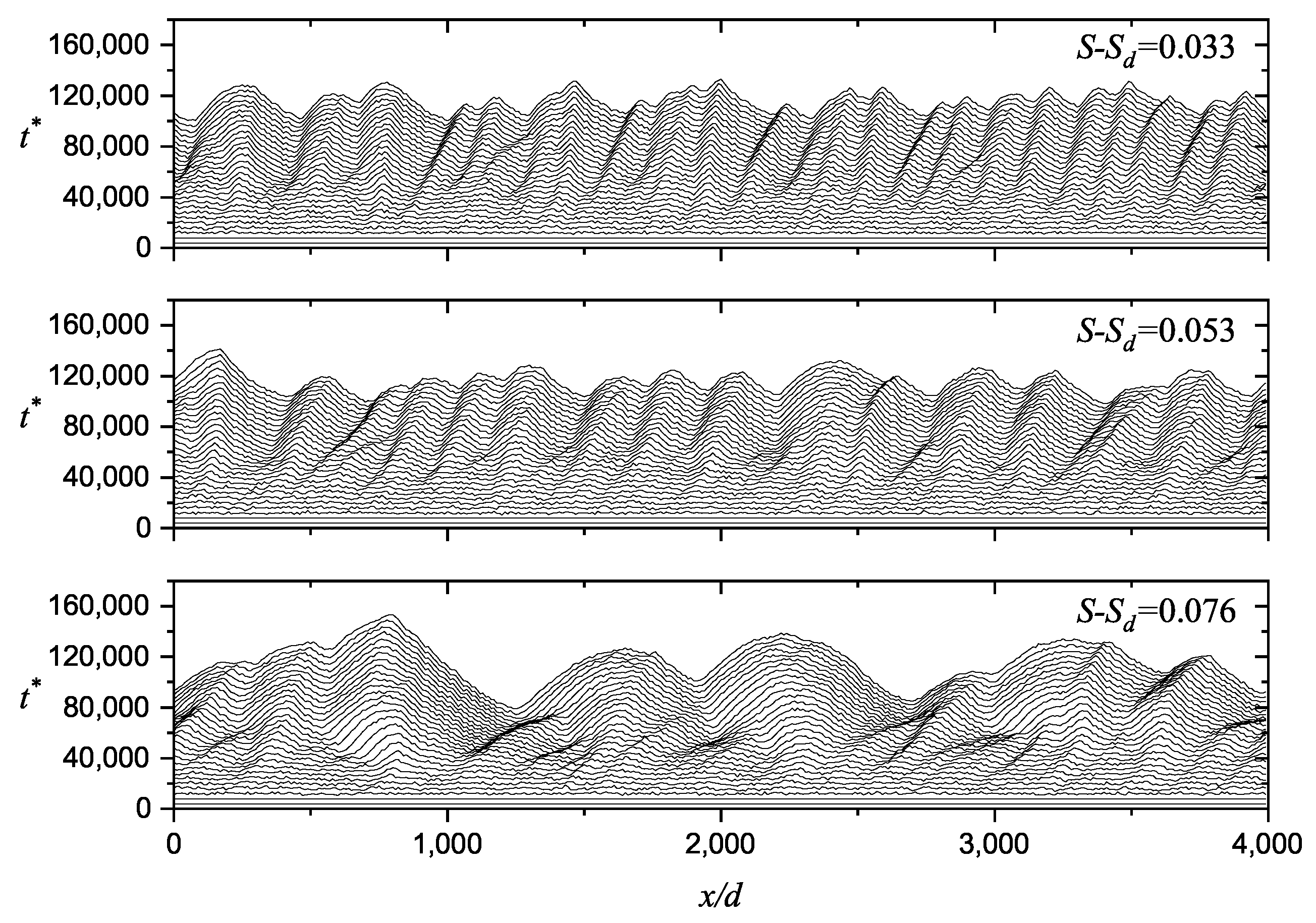
15) was unused during this time, and the sand flux rapidly reached to a steady value. We used this procedure to make sure that the following sand flux variation was only caused by the surface deformation. Then, the surface started to deform. As the space–time diagrams show in
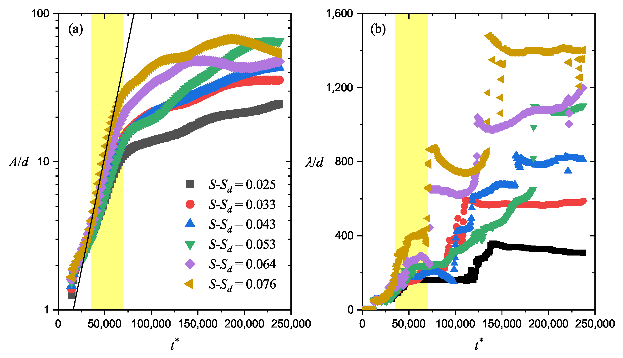
Figure 2, small bumps emerged from the sand bed regularly and migrated slowly in the wind direction. It is obvious that the wavelength (
, the horizontal distance from crest to crest) and the amplitude (
A, the vertical distance from trough to crest) of ripples grew with time. To have a clearer look at the morphological development of sand ripples, we calculated the autocorrelation
of the ripple profiles and averaged the results over the
y direction. Then, the average amplitude was calculated from
, and the average wavelength
corresponds to the x-coordinate of the first peak on
. As the results show in
Figure 3, the ripple wavelength and the amplitude both increased with time. Moreover, the growth rate became more and more insignificant, and it eventually became zero at the fully developed state of the aeolian sand ripples.
As the bright yellow background demonstrates, in
Figure 3a, there was a stage where the ripple amplitude grows exponentially. It is called the initial stage. Former works [
19,
30] have proved that before this stage (
35,000 in this work), the bed surface is noticeably three-dimensional. Small bumps emerge from the surface at an arbitrary location. These bumps grow in the transverse direction and link to each other. Eventually, they become the primitive form of aeolian sand ripples. Then, because of the symmetrical ripple form, the bed surface no longer varies in the
y direction. More and more low-energy particles tend to climb along the stoss slope of the sand ripple causing an exponential growth on the amplitude. From theoretical analyses, we have already known that this exponential-increase amplitude comes from the first-order contribution of the wavy bed surface [
11,
12,
15]. The most unstable mode of the surface profile caused by this contribution represents the initial wavelength, which corresponds to the first plateau of the wavelength in
Figure 3b. Then, after the initial stage (
70,000 in this work), coarsening takes place. It makes adjacent bumps merge to each other. We can see there was a continuous growth of the ripple wavelength in the initial stage and a subsequent step growth in the coarsening stage. The later abrupt wavelength growth was caused by merging ripples.
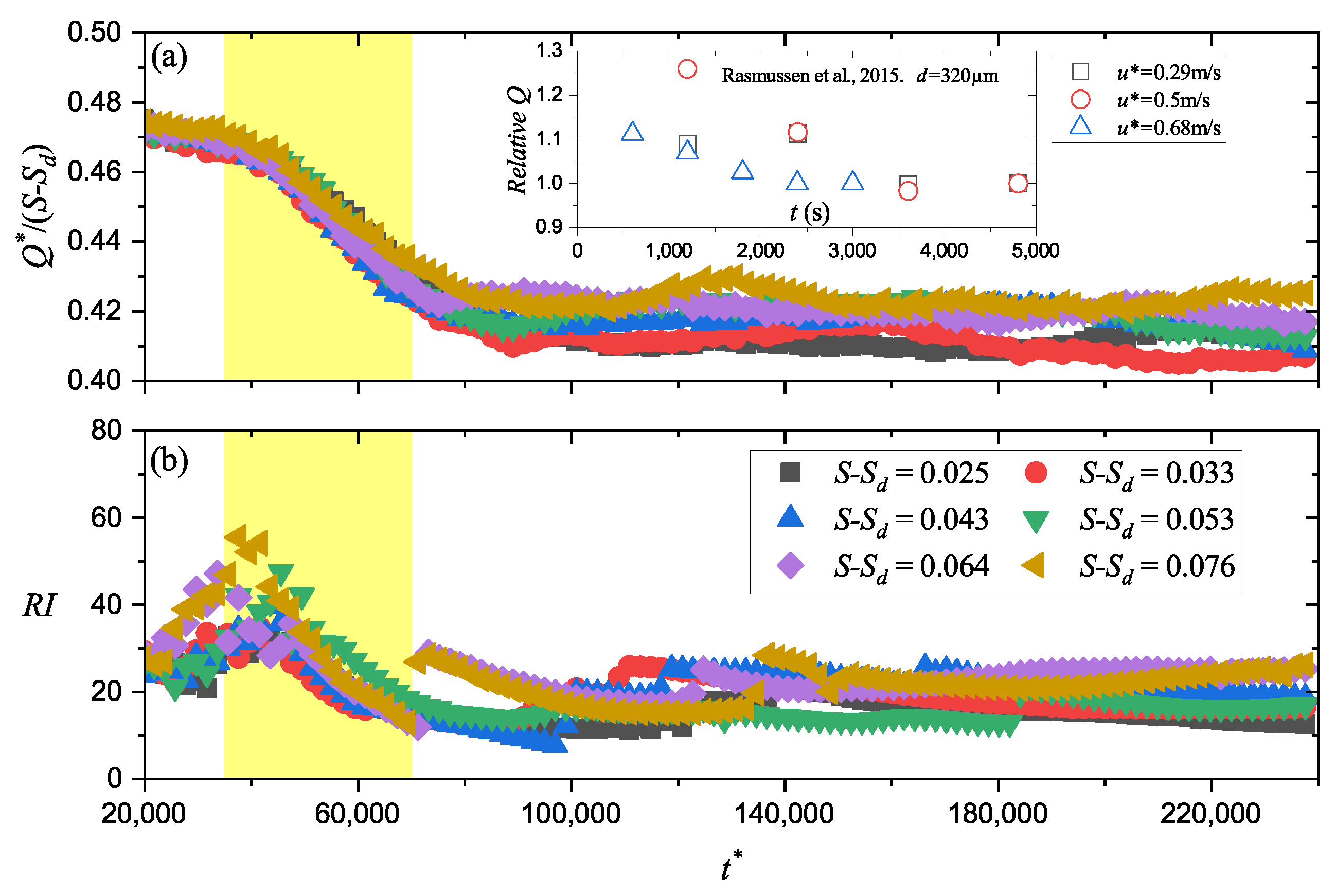
Next, we checked the sand flux variation during ripple formation. In this work, the horizontal sand flux
Q was calculated as the average horizontal particle momentum per unit bed area, i.e.,
, where
N is the particle number in the air;
is the bottom area of the entire computation domain; and
represents the time average. We nondimensionalized
Q via
. The temporal evolution of
in different wind strengths is shown in
Figure 4a. According to former experimental and numerical works [
19,
31,
32,
33], we have already known that there is a linear relationship between
Q and the Shields number
S. Thus, instead of
, here we checked
to reveal more information. It is worth mentioning that the threshold
used here was evaluated at
20,000. As the result shows,
holds a relatively stable value in the beginning of bed deformation. Then, an obvious decrease happens within the initial stage of the ripple formation. After the initial stage, a new stable value of
was reached. Except the decrease in sand flux, we noticed
derived from different wind strengths no longer coincided to each other after the initial stage. This can be caused by two possibilities: (a)
varies during the initial stage or (b) the relationship between
and
is not linear on the ripple surface. The latter is less likely to be true, because as we know, the linear relationship has already been proved by many experiments, which are always performed on ripple surface.
We also checked the temporal development of the ripple index (
) in
Figure 4b and found
increases until the initial stage begins. One needs to be aware that the value of
does not represent the ratio between
and
A before the initial stage. Because as mentioned before, the typical ripple form has not emerged at this time. Thus, the increase in
in this stage represents nothing, and the flux was unrelated to this variation until the initial stage. The sand ripple started to grow in the initial stage.
decreased in this stage, which is similar to
Q. This decrease lasted to the end of the initial stage, when
and
Q all reached to a relatively stable value. However, according to
Figure 3,
and
A held their increase after the initial stage. Thus, combining all the results, we can draw a conclusion that
Q is controlled by the ripple index
. Additionally, we noticed that the final
derived from our model was about 20. This coincides with the results from wind tunnel experiments and field observations [
1,
7,
9,
10]. However, they have not revealed the decrease in
within the initial stage.
3.2. The Relationship between the Sand Particle Transport and the Ripple Index
To perform further studies on the relationship between
Q and
, we ran several extra cases with pre-rippled sinusoidal wavy surfaces (triangular wavy surfaces and sinusoidal wavy surfaces showed no differences on the result). For all the cases, the amplitude
A was set as
, which is observed in
Figure 3a as a typical amplitude within the initial stage. The wavelength varies from
to
, making the ripple index
range from 6.25 to 125. The study on the situations with
was necessary, because for some specific conditions, the sand bed will develop to mega ripples, which has a much smaller ripple index [
34]. For every pre-rippled simulation case, the code module that contains Equation (
15) is disabled, and we reserved enough time for all the cases to ensure them to reach the saturated state. This procedure helped us to strictly control the value of
. To derive authentic results, for all the pre-rippled cases, the density ratio
s was set between 1325 and 5300;
ranged from 27 to 60; and
S varied from
to
. The other settings were the same as the settings of the ripple formation cases mentioned before.
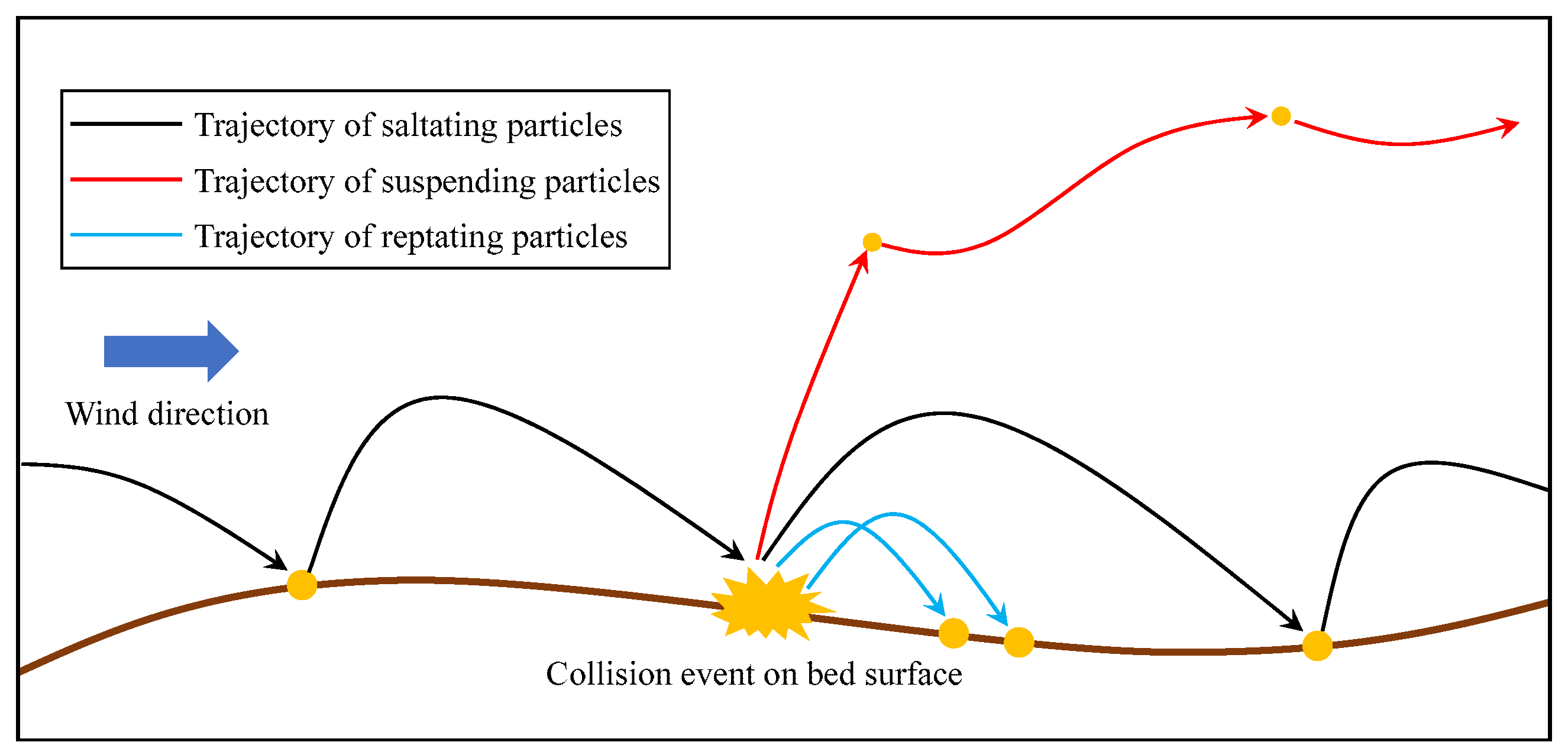
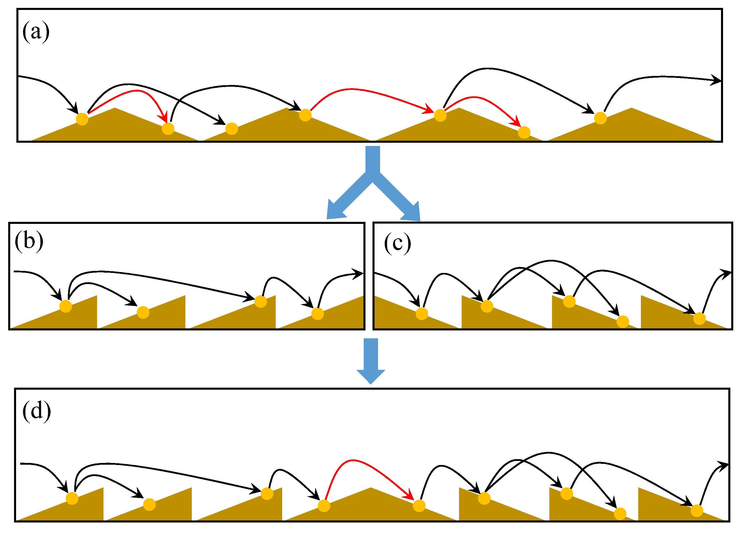
We first tried to simplify the problem. As
Figure 5a shows, reptating particles and saltating particles bounced forward along the wavy bed surface. There are two typical movement modes for them. One is hopping from a stoss slope to another stoss slope or from a lee slope to another lee slope (black lines in
Figure 5a demonstrate this kind of particle trajectories); the other one is hopping from a stoss slope to a lee slope or from a lee slope to a stoss slope (red lines in
Figure 5a demonstrate this kind of particle trajectories). We defined the former trajectories as monotone trajectories and defined the latter as non-monotone trajectories. As
Figure 5b,c shows, if all the particles have monotone trajectories and if we only study the ensemble average results, the whole system can be estimated by the combination of two simpler sub-systems, which only have a stoss slope or a lee slope. The particle with a non-monotone trajectory can be considered as a link, which transmits energy between the system shown in
Figure 5b,c. We checked this energy-transmitting capability by counting the particle number that impacts the surface or take-off from the surface.
represents the total number of impact particles that hit the stoss slope, and
represents the total number of the particles take-off from the stoss slope. Similarly, we also had
and
for the lee slope. We checked
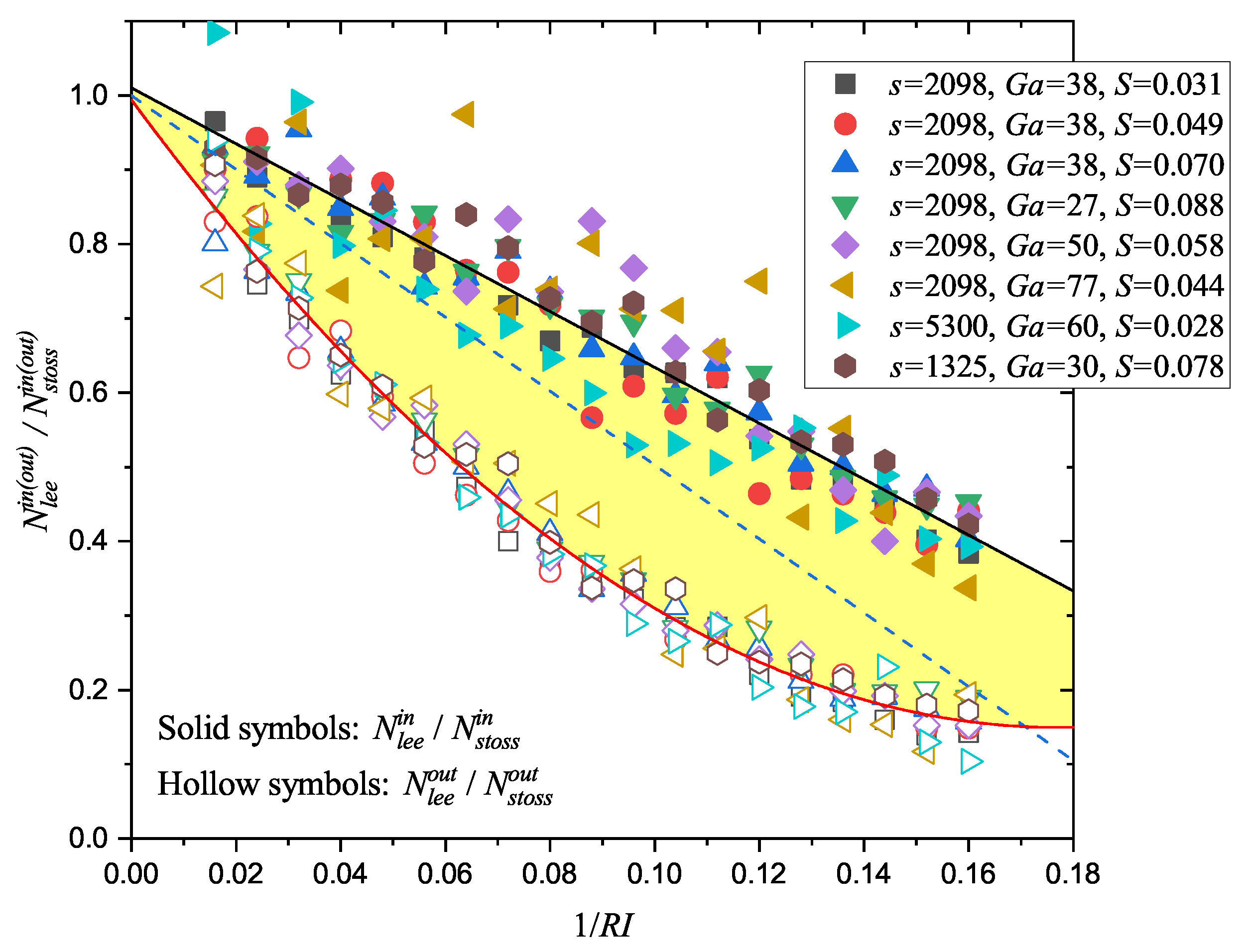
for the impact and take-off particles, because this ratio was useful for the subsequent studies. In
Figure 6, we found
decreased linearly with 1/RI, meanwhile,
decreased quadratically. These decreased relationships are all independent to the wind strength and the particle/fluid properties. Moreover, there was a difference between these two ratios, which is demonstrated by the bright yellow shade. This difference was due to the contribution of the non-monotone particle trajectories. Because if all particles have monotone trajectories, we can easily derive
and
. This yields an expression
where we defined this ratio as
. To continue our study, we adopted this simplification. For simplicity, we assumed
can be described by the linear fit of all the results in
Figure 6, which is demonstrated as the dashed line. Thus,
where
is a constant that will not change with the wind strength or the particle/fluid properties.
Similar to the definition of
Q, we defined the particle transport load
to represent the average total mass of particles transported above the bed surface per unit bed area. As
Figure 5 shows, we separated the whole system to two sub-systems. It is worth mentioning that these two sub-systems are not totally independent to each other. They share the same wind field. For a better understanding, one can imagine that we used the result derived from
Figure 5d to estimate the result in
Figure 5a. The former only has a few neglectable non-monotone trajectories in the middle. In the following work, for the particles interacting with the stoss slope, we used subscript
s to represent their statistical quantities. For the particles interacting with the lee slope, we used subscript
l. Then, we could write the stress balance on the bed surface [
35]
where
and
are horizontal and vertical grain-born stress applied on the bed surface, respectively. They arose from inter-particle or particle-bed contacts.
and
are slope angles. We assumed
.
is the air-borne shear stress far away from the bed surface;
is the air-borne shear stress on the bed surface. According to the drag partitioning theory [
36], for a saturatde wind-driven particle transport system,
, where
is the shear stress corresponding to the dynamic threshold. Moreover, recall the definition of
in Equation (
16); we find it can also represent the ratio of
M, i.e.,
. Use
, and define a parameter
. Then we can derive
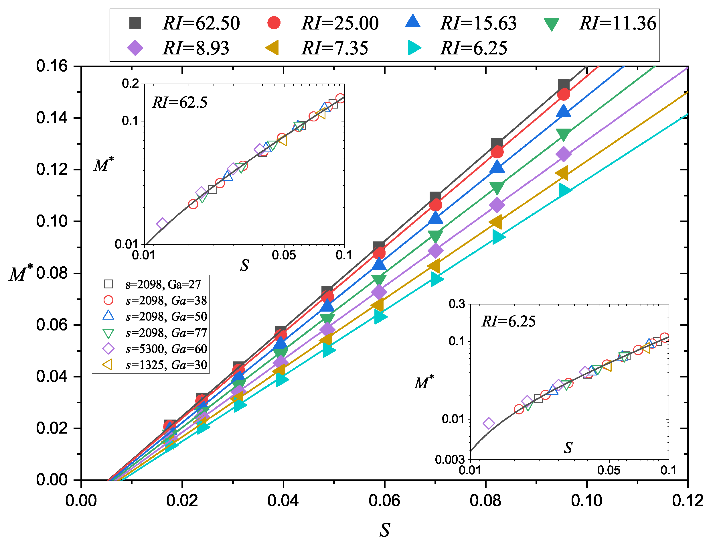
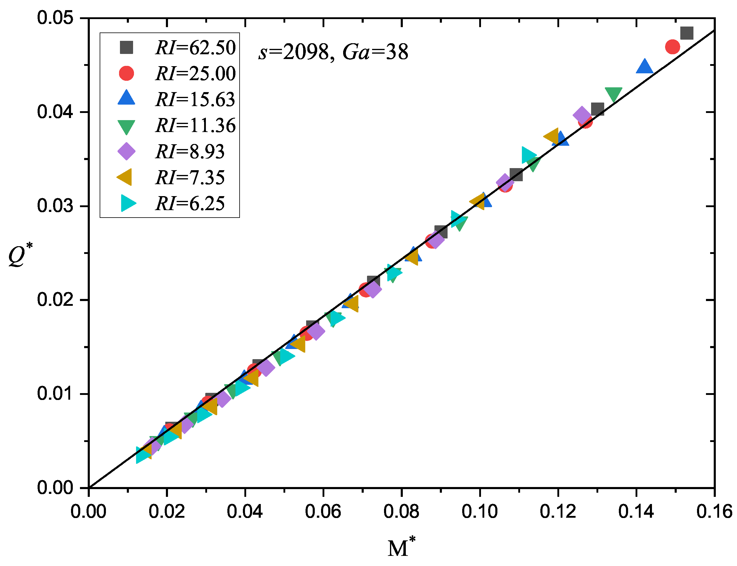
where
is the dimensionless form of
M;
. It shows a linear relationship between
and
S. From the simulation results shown in
Figure 7, we proved that
always holds for different
, different
s, and different
. Additionally, we found
is obviously influenced by
. The weak effect from
s can be observed from the result, as well. To obtain the relationship between
and
, we used
to roughly estimate the slope angle. Then, we have
which is derived from Equations (
17) and (
20).
As
Figure 7 shows, not only
varies with
;
also has a relationship with
. According to the
expressions on the slope [
28], we similarly scaled
as
Noticing that for the flat surface situation,
becomes an infinitely great value, which leads to
and
. Thus, according to Equations (
20) and (
21) with
, we can directly derive
and
from our flat surface results. It is worth mentioning that the “flat surface” here refers to the bed surface before the initial stage in the ripple formation simulation cases.
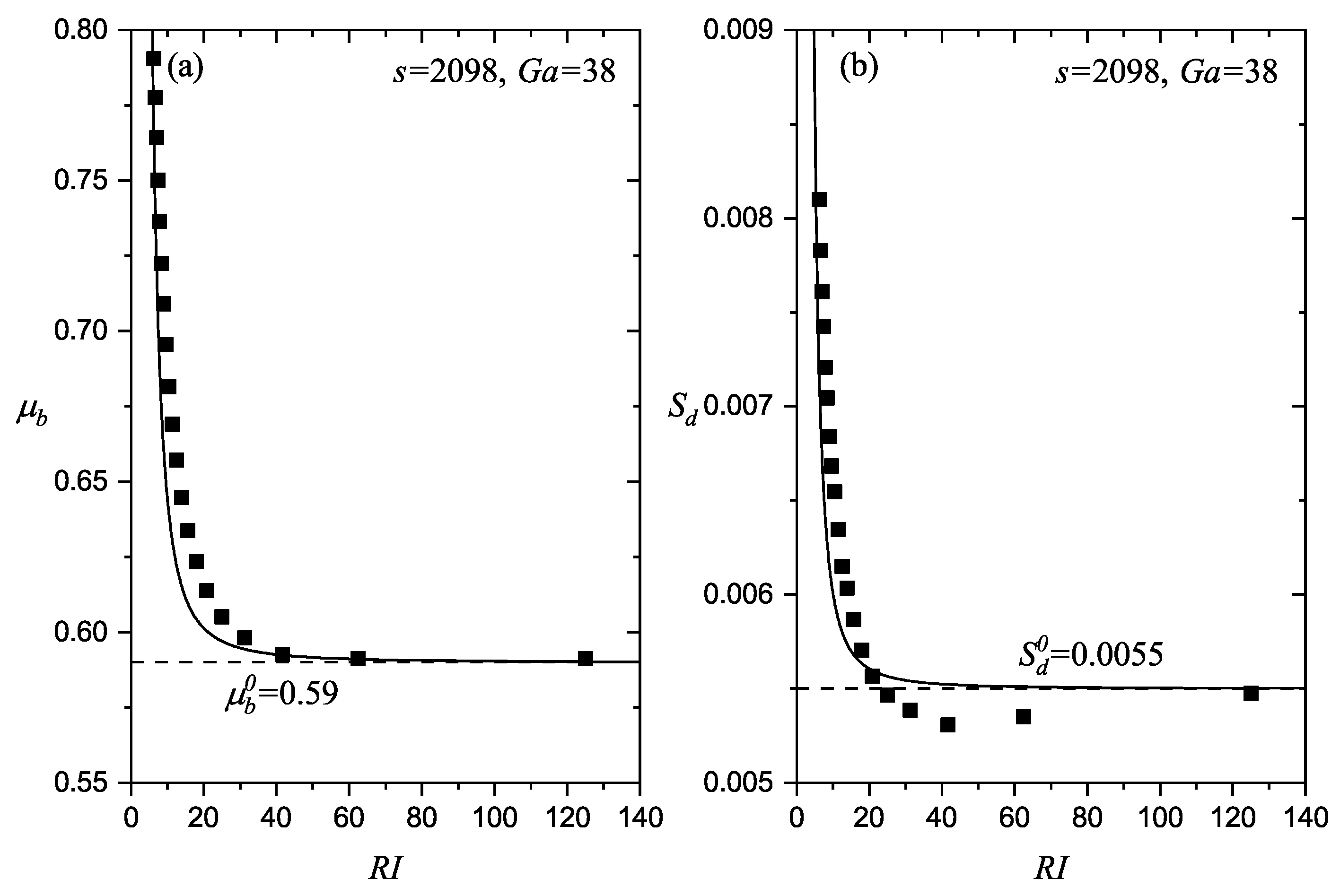
For the cases with
and
, we display the relationship between
and
in
Figure 8a.
decreased with
, and the decrease rate dropped rapidly.
became more and more close to
as
increased. The relationship between
and
had the similar rule (
Figure 8b). What was different was that the
first dropped to a value smaller than
at a large
. Then, as
continued growing, it gradually increased to the value close to
. With derived
and
, the results of Equations (
21) and (
22) are also shown in
Figure 8 as the solid lines. Both of them roughly fit the simulation results, but Equation (
22) cannot reflect the overly large decrease in
.
is the typical ripple index of the fully developed aeolian sand ripples on earth [
2,
9,
10]. According to our results, what varies most from the flat surface to
is not the dynamic threshold
but the parameter
. So, we can say
is a parameter that reflects the bed surface geometry. Substituting Equations (
21) and (
22) into Equation (
20), we obtained a brief expression of
where,
.
Finally, we checked the relationship between
and
. As
Figure 9 shows, with specific
s and
, for all the Shields numbers studied in this work (
), their relationship was close to linear. It is interesting that the ripple bed surface barely influenced the result. No obvious variations were observed between the results that corresponded to different
. Thus, the relationship
was still valid for the sand particle transport upon the ripple surface. What was different from the result on the flat surface was the dynamic threshold
, and the proportionality coefficient between
and
were controlled by the bed surface. According to Equation (
23), we can also scale
as
Using this expression, we can estimate the relative quantity of the sand flux decrease during aeolian sand ripple formation in wind tunnel experiments. On the flat surface, the dynamic threshold
can be estimated as
[
1,
37].
is the static threshold, and it can be calculated by
[
26]. Then, we can derive
. We used
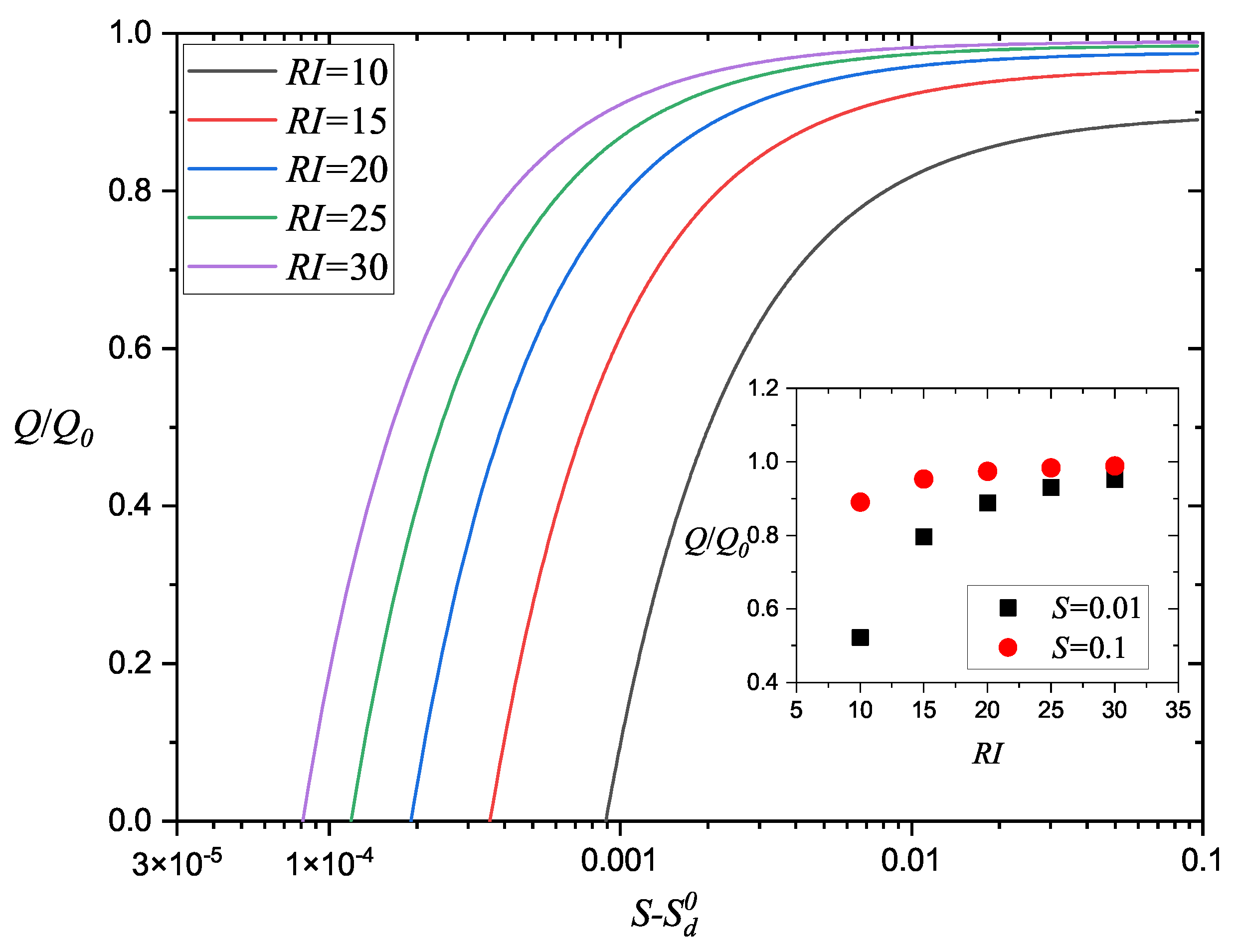
to represent the sand flux on flat surface. We easily derived
. We chose five common
, which varied from 10 to 30. These
represent different aeolian sand ripples that emerged in wind tunnel experiments.
Figure 10 exhibits the relationship between
and
S for a specific particle diameter
d = 250 μm. One can find that for a specific ripple index, the sand flux caused by small wind strength is easier to be influenced by the ripple surface.
rapidly approached to a constant value that was smaller than 1 when the wind strength increased. To have a clearer look, we extracted the
values that correspond to
and
. As shown in the inset of
Figure 10,
at these two wind strengths all increased with
. For all the
, the ripple bed was more influential to the sand flux in the situations with smaller wind strength. This coincides to the experiment result shown in the inset of
Figure 4a.


