Study of the Fluid Passing through the Screen in the Three Products Hydrocyclone Screen (TPHS): A Theoretical Analysis and Numerical Simulation

Abstract

The three products hydrocyclone screen (TPHS), a branch of the hydrocyclone, effectively removes the fish-hook effect, which has been used in the industrial field. The current cylindrical screen in the TPHS generates the characteristic flow known as the screen underflow, which has a significant impact on device performance. To investigate the flow behaviour of the fluid passing through the screen, a combination of a dynamic analysis and a numerical simulation was used. The permeating process in the TPHS was abstracted by a simple fan mode in this work to generate the flow-rate equations and the driving-force models. The pressure difference was the driving force for the screen penetration in the ideal fluid, but it also included a viscous force in the viscous fluid. Furthermore, at the same inlet velocity, the viscous fluid had a higher flow rate than the ideal, indicating that the viscosity promoted the fluid penetration. Meanwhile, as the inlet velocity increased, the mass flow of the screen backflow increased, while the corresponding proportion first rose to a peak then dropped and then gradually stabilised. Furthermore, a flow equation for the screen underflow in the TPHS was developed, which is related to the structural parameters (the rotation radius, the length of the cylindrical screen, the aperture size, and the open-area percentage) and the process parameters (the dynamic viscosity of the fluid and the pressure difference between the feed inlet and the screen outlet).

1. Introduction

Size separation is the process of dividing a group of particles into two or more size ranges based on their size, and it is widely used in many fields such as mining, the chemical industry, and environmental protection [1,2,3]. The three products hydrocyclone screen (TPHS) is an improved category of particle-classification equipment [4]. In the TPHS, a built-in cylindrical screen is adopted in a traditional cyclone, although there are simple structural changes. The TPHS separates the particles according to their sizes with the effect of the centrifugal classification and screening [5,6]. Due to the better device performance, including the higher Hancock classification efficiency, lower imperfection, and more reasonable cut size, the TPHS has been used in mineral engineering [7,8]. For example, in our previous study [7], the TPHS was successfully adopted in the Xuehu coal preparation plant, Henan, China. The application result showed that the size distribution of each product stream was optimised without increasing the complexity of the processing system due to the mixed overflow compared to the conventional hydrocylone. In addition, the TPHS showed that the imperfection (I) and the Hancock classification efficiency (HE) increased by ~0.08% and 11%, respectively, compared to the CH.

As an improved cyclone, the TPHS also shows complex flow behaviour. In previous works, the combination of the particle image velocimetry experiment and the computational fluid dynamics simulation was adopted to describe the fluid’s flow behaviour, pressure distribution, and turbulence characteristics [9,10]. In particular, the TPHS displays similar flow patterns to the hydrocyclone, such as a second circulatory flow, central down-flow, mantle, outer-downward swirl flow, and inner-upward swirl flow [11]. Besides, compared to the hydrocyclone, the TPHS shows a particular screen underflow, which results in a higher radial velocity and a lower tangential velocity [12,13]. These distinctions between the TPHS and the hydrocyclone can be attributed to the present cylindrical screen [14], which results in the entire elimination of the fish-hook effect. Thus, as the characteristic flow of the TPHS, the screen backflow significantly affects the device performance.

The above discussion means that some common comprehensions are effective with the TPHS. However, the details of the dynamic behaviour of the screen underflow were not reported and remain unexplored. Given this gap, new investigations adopting a numerical simulation were developed [10,12,14]. The dynamic analysis of the screen underflow was developed in this work to investigate the flow behaviour of the fluid passing through the screen using a simple model. The theoretical analysis models were then validated using a computational fluid dynamics (CFD) simulation. Finally, the valid models were extended to investigate the flow rate in the TPHS.

2. Methodology

In our earlier report, the numerical methods including the geometric models, numerical models, and simulation setup were verified step by step using a combination of the particle image velocimetry test and the CFD simulation [7,9,10]. As a series of studies for the TPHS, a valid methodology was considered in this work. The details are described as follows.

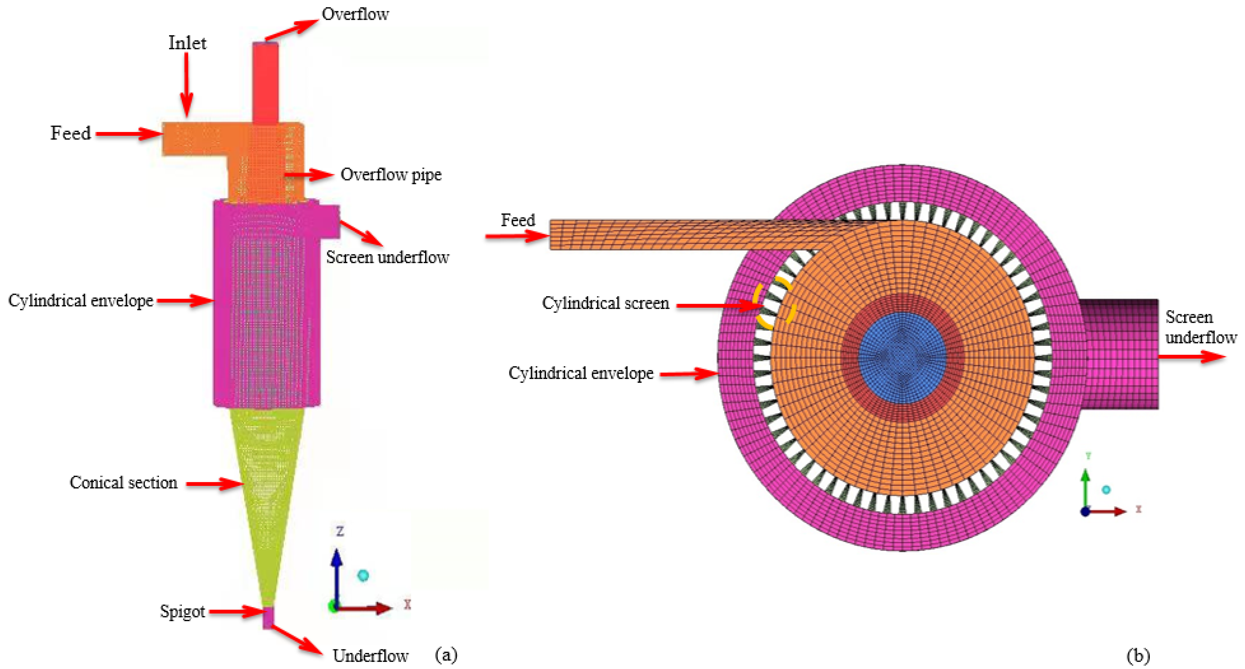
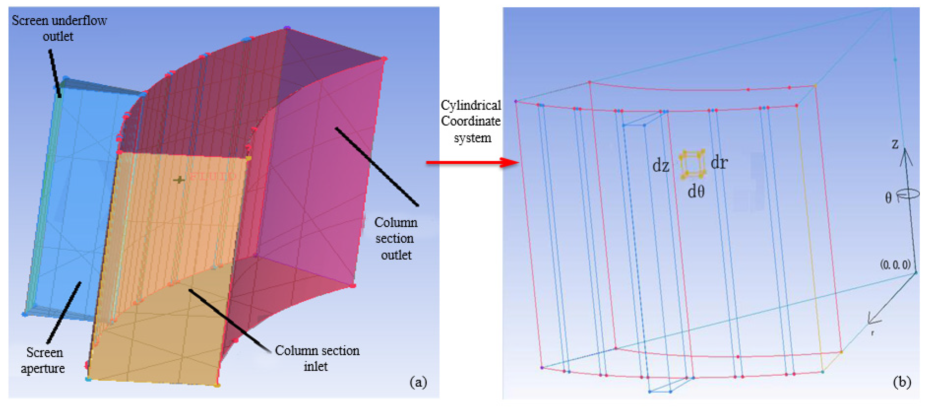
2.1. Geometric Models

This study took into account a 75 mm TPHS, whose diagrams are shown in Figure 1 (a) front view and (b) vertical view. In general, the TPHS is made up of a hydrocyclone, a cylindrical screen, a cylindrical envelope, inlet and outlets, and so on. The working principle of the TPHS is partially analogous to that of a conventional hydrocyclone. The slurry was measured at a velocity along the tangential inlet into the TPSH and was forced to move in a circular path by the geometry. In addition to the typical inner and outer spirals, the screen underflow was produced near the cylindrical screen in the TPHS [10]. This fluid behaviour was caused by the current screen, which clearly plays a role in improving the device performance. As a result, an abstract model was created to focus on the process of the fluid penetrating under the sieve, corresponding to the part of the yellow-dotted coil in Figure 1b that is shown in Figure 2a. In this model, a single screen and a fan channel with a rectangle inlet, rectangle outlet, screen aperture, and screen-underflow outlet were combined.

Table 1. Structure parameters of abstract fan models for TPHS.

Items	Abstract Fan Model
Radius of gyration	37.5 mm
Screen aperture size	0.7 mm
Thickness of screen bar	5 mm
Width of screen bar	3.25 mm
Length × Width of column-section inlet	29 mm × 8 mm
Length × Width of column-section outlet	29 mm × 8 mm

describes the specifics of each section. The fluid entered through the rectangle column-section inlet and exited through the same-size column-section outlet. Furthermore, some fluid was drained through the screen aperture due to the current screen aperture. Furthermore, the cylindrical coordinate system depicted in Figure 2b was assigned to study the fluid motion (see the details in Section 3.2).

Based on this model, the ANSYS ICEM 16.0 software package was used to generate the mesh. In detail, the mesh was designed based on the structured block, where the number of cells exceeded 0.18 million. The maximum cell skewness was below 0.8. The minimum quality was ~0.48. The minimum of the determination was ~0.6. In terms of our previous work [10], the above grid scheme can provide the economical grid-independence solution.

2.2. Numerical Models

In this study, the multiphase fluids were modelled by the VOF method [15,16]. The turbulence flow was described using the linear Reynolds Stress Model (RSM) [17,18] which is based on the Reynolds-Averaged Navier–Stokes (RANS) [19] equations. Moreover, the fluid behaviour in the near-wall region was modelled using the standard wall function. The numerical models are shown in

Table 2. Multiphase and turbulence models for CFD simulation.

Items	Models
Multiphase flow model
VOF equation:	$\frac{1}{{\rho }_q}\left[\frac{\partial }{\partial t}\left({\alpha }_q{\rho }_q\right)+\nabla \cdot \left({\alpha }_q{\rho }_q{\overrightarrow{u}}_q\right)={\displaystyle \sum _{p=1}^n\left({\stackrel{•}{m}}_{pq}-{\stackrel{•}{m}}_{qp}\right)}\right]$	(1)
	$\nabla =\frac{\partial }{\partial x}\overrightarrow{i}+\frac{\partial }{\partial y}\overrightarrow{j}+\frac{\partial }{\partial z}\overrightarrow{k}$	(2)
Turbulence model
Velocity:	$u_i=\overline{u_i}+u_i{}^{\prime }$	(3)
Continuity equation:	$\frac{\partial \rho }{\partial t}+\frac{\partial \rho }{\partial x_i}\left(\rho u_i\right)=0$	(4)
Motion equation:	$\frac{\partial }{\partial t}\left(\rho u_i\right)+\frac{\partial }{\partial x_j}\left(\rho u_i{u}_j\right)=-\frac{\partial p}{\partial x_i}+\frac{\partial }{\partial x_j}\left[\mu \left(\frac{\partial u_i}{\partial x_j}+\frac{\partial u_j}{\partial x_i}\right)\right]+\frac{\partial }{\partial x_j}\left(-\rho \overline{u_i^{\prime }{u}_j^{\prime }}\right)$	(5)
Linear RSMs:	$\begin{array}{l}\underset{\mathrm{Local} \mathrm{Time} \mathrm{Derivative}}{\underbrace{\frac{\partial }{\partial t}\left(\rho \overline{u_i^{\prime }{u}_j^{\prime }}\right)}}+\underset{{\mathrm{C}}_{\mathrm{IJ}}\equiv \mathrm{Convection}}{\underbrace{\frac{\partial }{\partial x_k}\left(\rho u_k\overline{u_i^{\prime }{u}_j^{\prime }}\right)}}\\ =\underset{D_{T,ij}\equiv \mathrm{Molecular} \mathrm{Diffusion}}{\underbrace{-\frac{\partial }{\partial x_k}\left[\rho \overline{u_i^{\prime }{u}_j^{\prime }{u}_k^{\prime }}+\overline{p^{\prime }\left({\delta }_{kj}{u}_i^{\prime }+{\delta }_{jk}{u}_j^{\prime }\right)}\right]}}-\underset{P_{ij}\equiv \mathrm{Stress} \mathrm{Production}}{\underbrace{\rho \left(\overline{u_i^{\prime }{u}_k^{\prime }}\frac{\partial u_j}{\partial x_k}+\overline{u_j^{\prime }{u}_k^{\prime }}\frac{\partial u_i}{\partial x_k}\right)}}\\ +\underset{{\mathsf{\Phi }}_{ij}\equiv \mathrm{Pressure} \mathrm{Strain}}{\underbrace{\overline{p\prime \left(\frac{\partial u_i^{\prime }}{\partial x_j}+\frac{\partial u_j^{\prime }}{\partial x_i}\right)}}}-\underset{{\epsilon }_{ij}\equiv \mathrm{Dissipation}}{\underbrace{2\mu \overline{\frac{\partial u_i^{\prime }}{\partial x_k}\frac{\partial u_i^{\prime }}{\partial x_k}}}}\end{array}$	(6)
	$\begin{array}{l}{\mathsf{\Phi }}_{ij}=-1.8\rho \frac{\epsilon }{k}\left[\overline{u_i^{\prime }{u}_j^{\prime }}-\frac{2}{3}{\delta }_{ij}k\right]-0.6\left[\left(P_{ij}-C_{ij}\right)-\frac{1}{3}{\delta }_{ij}\left(P_{kk}-C_{kk}\right)\right]\\ -\frac{0.294\sqrt{k}}{d}\left(\overline{u_i^{\prime }{u}_k^{\prime }}{n}_j{n}_k+\overline{u_j^{\prime }{u}_k^{\prime }}{n}_i{n}_k\right)-\frac{0.176k^{1.5}}{\epsilon d}\left({\varphi }_{ik,2}{n}_j{n}_k+{\varphi }_{jk,2}{n}_i{n}_k\right)\end{array}$
Standard wall function:	$\frac{U_P{0.09}^{1/4}{k}_P^{1/2}}{{\tau }_w/\rho }=\frac{1}{0.4187}\ln \left(9.793\frac{\rho {0.09}^{1/4}{k}_P^{1/2}{y}_P}{\mu }\right)$	(7)

. Note that all the variables are interpreted in the section Nomenclature.

Water and air were chosen as the major and secondary fluid phases in this study, respectively. The feed was assumed to have a velocity inlet of 0~20 m/s, while all the discharge ports were assumed to have a pressure outlet of 1 atm, i.e., the ambient atmospheric pressure. Meanwhile, each outlet’s reflux air volume fraction was 1. The hydraulic diameter was set to be the characteristic size of each opening, and the turbulence intensity was set to 5%. For the standard initialisation, the air fraction of all of the zones was set to 1. The time step and the maximum iteration step were both 0.001 s. Furthermore, the tolerance of each equation was set to 10⁻⁶. The simulation was calculated to 20 s for the time-independent solution in each case. Finally, all convergent results were obtained on a higher-performance computer equipped with sixteen CPUs.

3. Results and Discussion

3.1. Dynamic Analysis of Screen Underflow

The screen underflow had a significant impact on the fluid flow in the equipment because of the TPHS characteristic flow. The dynamic analysis of the fluid permeability behaviour was performed to elucidate the formation mechanism of this flow behaviour and the determinants of the permeable flow rate. As mentioned in Figure 2 above, the abstract fan model was assigned. According to the N-S equation for the incompressible fluid in the cylindrical coordinate system, the equation of the fluid microelement dv (dr × dθ × dz) (see the orange cube in Figure 2) located on any flow radius (r) is obtained, shown in Equations (8) and (9). It is noted that the r, θ, and z are the variables in the cylindrical coordinate system, which means the radius, rotation angle, and axial, respectively.

$$\begin{array}{l}\frac{d{u}_r}{dt}=f_r-\frac{1}{\rho }\frac{\partial p}{\partial r}+\upsilon (\frac{1}{r}\frac{\partial }{\partial r}(r\frac{\partial u_r}{\partial r})-\frac{u_r}{r^2}+\frac{1}{r^2}\frac{{\partial }^2{u}_r}{\partial {\theta }^2}-\frac{2}{r^2}\frac{\partial u_{\theta }}{\partial \theta }+\frac{{\partial }^2{u}_r}{\partial z^2})\\ \frac{d{u}_{\theta }}{dt}=f_{\theta }-\frac{1}{\rho r}\frac{\partial p}{\partial \theta }+\upsilon (\frac{1}{r}\frac{\partial }{\partial r}(r\frac{\partial u_{\theta }}{\partial r})-\frac{u_{\theta }}{r^2}+\frac{1}{r^2}\frac{{\partial }^2{u}_{\theta }}{\partial {\theta }^2}+\frac{2}{r^2}\frac{\partial u_r}{\partial \theta }+\frac{{\partial }^2{u}_{\theta }}{\partial z^2})\\ \frac{d{u}_z}{dt}=f_z-\frac{1}{\rho }\frac{\partial p}{\partial z}+\upsilon (\frac{1}{r}\frac{\partial }{\partial r}(r\frac{\partial u_z}{\partial r})+\frac{1}{r^2}\frac{{\partial }^2{u}_r}{\partial {\theta }^2}-\frac{2}{r^2}\frac{{\partial }^2{u}_z}{\partial {\theta }^2}+\frac{{\partial }^2{u}_z}{\partial z^2})\end{array}\}$$

(8)

$$p=(p_{rr}+p_{\theta \theta }+p_{zz})/3$$

(9)

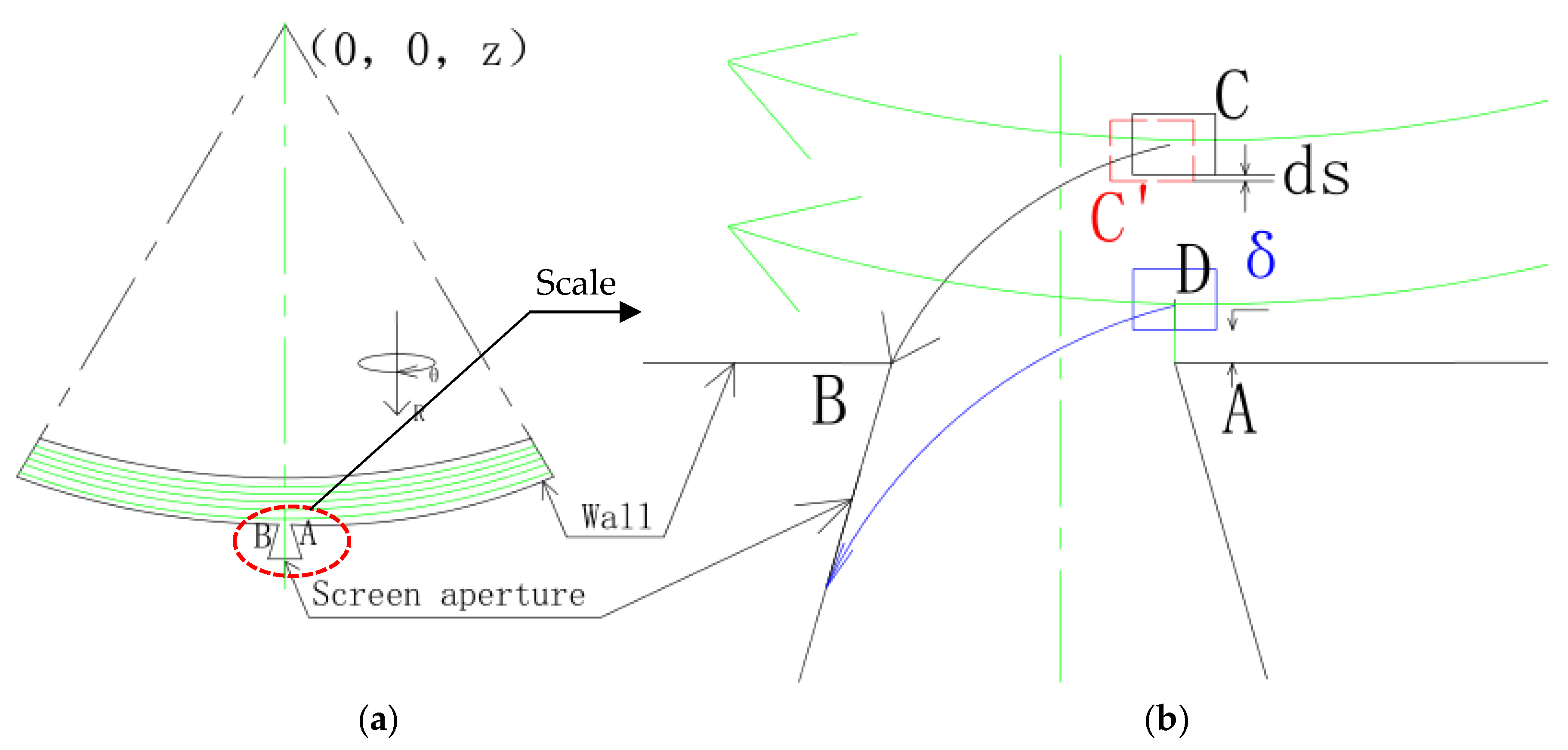
3.1.1. Analysis of Ideal Fluid Permeability Sieve

According to the particularity of the fluid-screening process in the TPHS and the simple model, the following assumptions were taken:

(1)

the fluid was ideal with the kinematic viscosity υ of 0 m²/s;

(2)

the fluid-permeable screen can be considered as the fluid passing through the inner surface of the screen (namely the small end of the cone frustum in Figure 2b);

(3)

the process of permeating the screen was the result of the fluid migration in the radial and tangential directions; thus, the axial flow can be ignored.

Thus, the 3D spatial flow shown in Figure 2 can be converted to the 2D plane flow shown in Figure 3. Meanwhile, the following formulas can be obtained:

$$\begin{array}{l}\frac{d{u}_r}{dt}=f_r-\frac{1}{\rho }\frac{\partial p}{\partial r}\\ \frac{d{u}_{\theta }}{dt}=f_{\theta }-\frac{1}{\rho r}\frac{\partial p}{\partial \theta }\end{array}\}$$

(10)

$$p=(p_{rr}+p_{\theta \theta })/2$$

(11)

Figure 3a depicts the 2D plane flow as an axial-plane z of the 3D spatial flow depicted in Figure 2b,c. The corresponding scale diagram near the screen aperture is shown in Figure 3b (see the red-dotted line in Figure 3a). Figure 3 depicts (b), it presents the class of the flat parabolic motion to any fluid microelement dv (drd) perpendicular to Position A, viz., the flow-permeating behaviour was composed of the radial and tangential motion. For example, the fluid microelement D (shown in blue in Figure 3b) moved along the blue trace line via the screen. In the worst-case scenario, the fluid only moves to the inner surface of the screen’s end (i.e., Point B). Between these two possibilities, the fluid may or may not pass through the screen.

Take the variables $u_r$, $u_{\theta }$ as the radial and tangential velocity of the fluid microelement, respectively. Moreover, set D as the width of the screen aperture. Noted that the value of D (~0.65 mm) was smaller than that of the rotation radius r (37.5 mm), thus the short-arc segment from A to B can be treated as a straight line.

Along the radial direction, the fluid microelement dv (see the black rectangle in Figure 3) moved from the moment t₁ (Position C) to the moment t₂ (Position C′). For this process, according to Newton’s second law, the following Equation can be obtained:

$$ds=v_{r}dt+\frac{1}{2}{a}_r{(dt)}^2=v_{r}dt+\frac{1}{2}\frac{d{u}_r}{dt}{(dt)}^2$$

(12)

where the variable ds is the displacement along the radial direction. Bring Equation (10) into Equation (12):

$$ds=v_{r}dt+\frac{1}{2}(f_r-\frac{1}{\rho }\frac{\partial p}{\partial r}){(dt)}^2$$

(13)

Therefore, take the integral:

$${\displaystyle {\int }_{r_1}^{r_2}ds}={\displaystyle {\int }_{t_1}^{t_2}{v}_{r}dt}+{\displaystyle {\int }_{t_1}^{t_2}\frac{1}{2}(f_r-\frac{1}{\rho }\frac{\partial p}{\partial r}){(dt)}^2}$$

(14)

Then, solve Equation (14):

$$\mathsf{\Delta }s={\displaystyle {\int }_{r_1}^{r_2}ds}={s|}_{r_1}^{r_2}=r_2-r_1$$

(15)

$${\displaystyle {\int }_{t_1}^{t_2}{v}_{r}dt}+{\displaystyle {\int }_{t_1}^{t_2}\frac{1}{2}(f_x-\frac{1}{\rho }\frac{\partial p}{\partial r})d{t}^2}={v_{r}t|}_{t_1}^{t_2}+\frac{1}{2}(f_x-\frac{1}{\rho }\frac{\partial p}{\partial r}){t^2|}_{t_1}^{t_2}$$

(16)

Assume Position C is the initial time, i.e., t₁ = 0, then:

$$\mathsf{\Delta }s=r_2-r_1=v_r{t}_2+\frac{1}{2}(f_r-\frac{1}{\rho }\frac{\partial p}{\partial r})t_2{}^2$$

(17)

Considering the above limit condition in Figure 3b, when the fluid moved exactly to the Position B:

$$\mathsf{\Delta }t=t_2-t_1=t_2=\frac{D}{v_{\theta }}$$

(18)

Combine Equations (17) and (18):

$$\begin{array}{l}\mathsf{\Delta }s=v_r\frac{D}{v_{\theta }}+\frac{1}{2}(f_r-\frac{1}{\rho }\frac{\partial p}{\partial r}){(\frac{D}{v_{\theta }})}^2\\ =\frac{v_r}{v_{\theta }}D+\frac{1}{2}{f}_r{(\frac{D}{v_{\theta }})}^2+\frac{1}{\rho }{(\frac{D}{v_{\theta }})}^2\frac{-\partial p}{\partial r}\end{array}$$

(19)

Due to the width of the screen aperture being small, the tangential velocities $v_{\theta }$ during the above permeating process can be considered to remain constant. In Figure 3b, set the variable Δ as the distance from the fluid microelement to the wall. Assume that Δ is equal to Δs which implies the limit distance of the fluid-penetrating screen. Namely, only the fluid within this distance can pass through the screen, and vice versa. Based on this, the flow rate q in the 2D plane flow can be calculated:

$$\begin{array}{l}q=\mathsf{\Delta }s\ast v_{\theta }=(\frac{v_r}{v_{\theta }}D+\frac{1}{2}{f}_r{(\frac{D}{v_{\theta }})}^2+\frac{1}{\rho }{(\frac{D}{v_{\theta }})}^2\frac{-\partial p}{\partial r})v_{\theta }\\ =v_{r}D+{\frac{f_{r}D}{2v_{\theta }}}^2+\frac{D^2}{\rho v_{\theta }}\frac{-\partial p}{\partial r}\end{array}$$

(20)

From the 2D plane flow to the 3D spatial flow, the flow rate $dq$ can be obtained:

$$dq=\mathsf{\Delta }s\ast v_{\theta }\ast dz=(v_{r}D+{\frac{f_{r}D}{2v_{\theta }}}^2+\frac{D^2}{\rho v_{\theta }}\frac{-\partial p}{\partial r})dz$$

(21)

Take the integral:

$${\displaystyle \int dq}={\displaystyle \int \mathsf{\Delta }s\ast v_{\theta }\ast dz}={\displaystyle \int (v_{r}D+{\frac{f_{r}D}{2v_{\theta }}}^2+\frac{D^2}{\rho v_{\theta }}\frac{-\partial p}{\partial r})dz}$$

(22)

Set the integral interval of z as the variable H, then:

$$\mathsf{\Delta }q=\mathsf{\Delta }s\ast v_{\theta }\ast H=(\underset{\mathrm{Initial} \mathrm{speed} \mathrm{item}}{\underbrace{v_{r}D}}+\underset{\mathrm{Mass} \mathrm{force} \mathrm{item}}{\underbrace{{\frac{f_{r}D}{2v_{\theta }}}^2}}+\underset{\mathrm{Pressure} \mathrm{item}}{\underbrace{\frac{D^2}{\rho v_{\theta }}\frac{-\partial p}{\partial r}}})H$$

(23)

For the present simple model (in Figure 2a), the value of H is equal to the height of the column-section inlet H (29 mm). Equation (23) is the calculation for the flow rate of the ideal fluid passing through the screen. It can be seen that the permeating fluid was determined by the initial radial velocity, mass force, and pressure difference. Change Equation (23):

$$\mathsf{\Delta }q=\mathsf{\Delta }s\ast v_{\theta }\ast H=(\frac{v_r}{v_{\theta }}+\frac{D{f}_r}{2v_{\theta }{}^2}+\frac{D}{\rho v_{\theta }{}^2}\frac{-\partial p}{\partial r})D{v}_{\theta }H$$

(24)

where $\frac{v_r}{v_{\theta }}$, $\frac{D{f}_r}{2v_{\theta }{}^2}$, $\frac{-\partial P}{\partial r}\frac{D}{\rho v_{\theta }{}^2}$, can be known as the dimensionless coefficients. In terms of the previous work, the mass force can be ignored in the centrifugal force field:

$$\mathsf{\Delta }q\approx (\frac{v_r}{v_{\theta }}+\frac{D}{\rho v_{\theta }{}^2}\frac{-\partial p}{\partial r})D{v}_{\theta }H$$

(25)

Similarly, Equation (10) can be replaced by the following expression:

$$\frac{d{u}_r}{dt}\approx -\frac{1}{\rho }\frac{\partial p}{\partial r}$$

(26)

From this equation, it can be seen that the pressure gradient near the screen is the driving force for the fluid passing through the screen.

3.1.2. Analysis of Viscous Fluid Permeability Sieve

For the actual fluid, the viscous effect should be considered, thus, the kinematic viscosity $\upsilon$ in Equation (8) cannot be ignored. Then, referring to the above derivation process of the ideal fluid, the following Equation (27) was obtained, where $\mathsf{\Delta }{q}^{\prime }$ represents the flow rate permeating the screen for the viscous fluid:

$$\mathsf{\Delta }{q}^{\prime }=\mathsf{\Delta }{s}^{\prime }{v}_{\theta }H\approx (\frac{v_r}{v_{\theta }}+\frac{D}{\rho v_{\theta }{}^2}\frac{-\partial p}{\partial r}+\frac{f_{\mu }}{D})D{v}_{\theta }H$$

(27)

$$\frac{d{u}_r}{dt}\approx -\frac{1}{\rho }\frac{\partial p}{\partial r}$$

(28)

Comparing Equations (25) and (27), it is clear that the sieving process of the viscous fluid is affected by the fluid viscous force in addition to the fluid pressure gradient compared to the ideal fluid, and the sieving volume of the viscous fluid is larger than that of the ideal fluid under the same conditions.

3.2. Verification by Simulation

As stated in Section 2.2, the numerical experiments using a combination of VOF and the RSM were accepted to validate the above theoretical equation. It should be noted that the effectiveness of the aforementioned numerical models was demonstrated in previous works.

The inlet velocity in the current simulation was 0~20 m/s. Where other velocities were comparable, the feed velocity of 1 m/s was chosen for the following analysis. The velocity vectors of the simple models of the (a) ideal and (b) viscous fluid, with an inlet velocity of 1 m/s, are shown in Figure 4. The fluid clearly flowed along the channel in this figure, but due to the current screen aperture, the fluid passed through the screen to generate the screen underflow. The fluid velocity remained relatively stable in the main channel (i.e., the arc channel), but changed rapidly near the screen aperture. This is due to the formation of the screen backflow. In detail, due to the blockage of the screen wall, the tangential velocity of the screen underflow rapidly decreased to 0 m/s, quickly converted to the radial velocity, and then quickly discharged via the screen-underflow outlet. With this change in flow velocity, the fluid experienced a rapid conversion between dynamic and static pressure. In comparison to Figure 4a,b, the ideal fluid exhibited a greater radial velocity over a longer distance, whereas the viscous fluid exhibited a larger velocity gradient with an obvious vortex along the vertical screen wall. The presence of the vortex increased the energy consumption while decreasing the radial velocity.

Figure 5 depicts the distribution of (a) the mass flow and (b) the screen under flow for the ideal and viscous fluids at different inlet velocities (120 m/s). This proportion denotes the mass percentage of the screen underflow in the feed. The fluid permeability flow rate was proportional to the feed rate, as shown in Figure 5a. Furthermore, the permeability flow rate of the viscous fluid was greater than the permeability flow rate of the ideal fluid. The proportion of the screen underflow of the viscous fluid was clearly greater than that of the ideal fluid in Figure 5b. The trends in Figure 5a,b show that the viscosity was favourable for passing through the screen.

Furthermore, when comparing Figure 5a,b, it is clear that increasing the inlet velocity from 0~20 m/s increased the mass flow of the screen underflow, but the percentage of the screen underflow showed different trends. In particular, as the inlet velocity increased, both the ideal and viscous fluid showed a similar distribution, i.e., the percentage of the screen underflow first rose to a peak, then fell, and then finally remained stable. This shows that, while the mass flow of the screen backflow increased with the increasing inlet velocity, the corresponding proportion increased first, then decreased and presented the peak value.

When multiple screen apertures are present along the fluid movement direction, the fluid permeation behaviour can be viewed as the sum of the fluid permeation behaviour in each screen aperture. Thus, 50 screen apertures were used to model the geometry in the CFD simulation of the fluid permeation under multiple screen aperture conditions. The numerical models for the multi-aperture screens were similar to those for the single screens. Figure 6 depicts a velocity vector with multiple apertures for (a) the viscous and (b) the ideal fluids with an inlet velocity of 1 m/s. At the same velocity inlet, the fluid velocity gradually decreased along the flow direction. Furthermore, the viscous fluid decelerated faster than the ideal fluid.

Figure 7 depicts the distribution of the two fluids’ screen underflow diversion ratios at different screen apertures along the rotation direction. The viscous fluid had a higher screen underflow diversion ratio than the ideal fluid at any screen aperture in Figure 7, with the former having a total screen underflow diversion ratio of 34.92 percent and the latter 19.78 percent at all of the screen apertures. Similarly, the proportion away from an inlet (i.e., the lower tangential velocity) was greater than the proportion near the feed (namely the higher tangential velocity). This is comparable to the above distribution of a single screen at various inlet velocities.

At the small flow rate, it is higher than that at the large flow rate, which is similar to the rule that the larger the inlet flow rate of a single screen slit, the smaller the screen underflow diversion ratio.

3.3. Flow Equation of Screen Underflow

The above study displayed that the flow rate (see the details in Section 3.1) is valid to the simple model. To extend this to the TPHS, the following analysis was conducted.

In Equation (27), for any screen aperture, assume the above dimensionless coefficients $\frac{v_r}{v_{\theta }}$, $\frac{-\partial P}{\partial r}\frac{D}{\rho v_{\theta }{}^2}$, $\frac{f_{\mu }}{D}$:

$$\begin{array}{l}\frac{v_r}{v_{\theta }}=c_1\frac{D}{\rho v_{\theta }{}^2}\frac{-\partial p}{\partial x}\\ \frac{f_{\mu }}{D}=c_2\frac{D}{\rho v_{\theta }{}^2}\frac{-\partial p}{\partial x}\end{array}\}$$

(29)

Equation (24) can be transformed:

$$\mathsf{\Delta }{q}^{\prime }=(c_1+1+c_2)\frac{D}{\rho v_{\theta }{}^2}\frac{-\partial p}{\partial x}D{v}_{\theta }H$$

(30)

where $c_1$ and $c_2$ are the relationship coefficients. Let $c_3=v_{\theta }/v_r$, and then from Equation (30), the following expression was obtained:

$$\frac{-\partial p}{\partial x}=\frac{1}{(c_1+1+c_2)}\frac{\mathsf{\Delta }q(\rho v_{\theta }l)}{(Dl)(DH)}=\frac{c_3}{(c_1+1+c_2)}\frac{\mathsf{\Delta }q(\rho v_{r}l)}{(Dl)(DH)}$$

(31)

where $l$ is the length of the screen aperture. The fluid Reynolds number in the screen ($R{e}_{\mathrm{aperture}}$) can be expressed as:

$$R{e}_{\mathrm{aperture}}=\frac{l\rho v_r}{\mu }$$

(32)

Then substitute Equation (32) into Equation (31):

$$\frac{-\partial p}{\partial x}=\frac{c_{3}R{e}_{\mathrm{aperture}}}{(c_1+1+c_2)}\frac{\mathsf{\Delta }q\mu }{(Dl)(DH)}=c_4\frac{\mu \mathsf{\Delta }q}{kA}R{e}_{\mathrm{aperture}}$$

(33)

Let $c_4=c_3/(c_1+1+c_2)$, A = DH, k = Dl, then:

$$\frac{-\partial p}{\partial x}=c_4\frac{\mu \mathsf{\Delta }q}{kA}R{e}_{\mathrm{aperture}}$$

(34)

where μ is the dynamic viscosity. Equation (33) is highly similar to Darcy’s law [20], both in terms of the magnitude and the form of the equation. Referring to L.G.M. Vieira et al. [21,22] for the solution of the filtered fluid flow in the column-coordinate system, the following Equation can be obtained:

$$\mathsf{\Delta }q=\frac{1}{c_4}\frac{kA}{R{e}_{\mathrm{aperture}}\mu l}\mathsf{\Delta }P$$

(35)

Equation (35) presents the flow rate for a single screen, then extends it to the TPHS. Let R and γ be the radius and the open-area percentage of the cylindrical screen, then the flow rate for the TPHS is developed:

$$\mathsf{\Delta }{q}_{TPHS}=\frac{1}{c_4}\frac{2\pi RH\gamma k}{R{e}_{\mathrm{aperture}}\mu l}\mathsf{\Delta }{P}^n=\frac{2\pi }{c_{4}R{e}_{\mathrm{aperture}}}\frac{RH\gamma k}{\mu l}\mathsf{\Delta }{P}^n=c\frac{RHD\gamma }{\mu }\mathsf{\Delta }{P}^n$$

(36)

where c is a parameter related to the fluid permeability and n is the pressure index. This expression reveals that the flow rate of the screen underflow was determined by the structure and the process parameters. For a certain TPHS, take the pilot scale φ150 TPHS in our previous study, for example. R, H, D, γ and μ correspond to the rotation radius (i.e., half of the diameter) of the TPHS (0.075 m), the length of the cylindrical screen (0.37 m), the aperture size (0.7 × 10⁻³ m), the open-area percentage (24%), and the dynamic viscosity of water (0.001 N·s/m²), respectively. ΔP is the pressure difference between the feed inlet and screen outlet, which can be obtained by a manometer, while c and n can be obtained by a series of experiments.

4. Conclusions

The three production hydrocyclone screen (TPHS) is designed for particle classification based on size and has been used in the industrial field. Because of the current cylindrical screen in the TPHS, the screen underflow can be regarded as the specific flow behaviour that prominently promotes the classification effect. The flow behaviour of the fluid passing through the screen was investigated using a combination of a dynamic analysis and a numerical simulation. From the above investigation, the following conclusions were obtained:

(1)

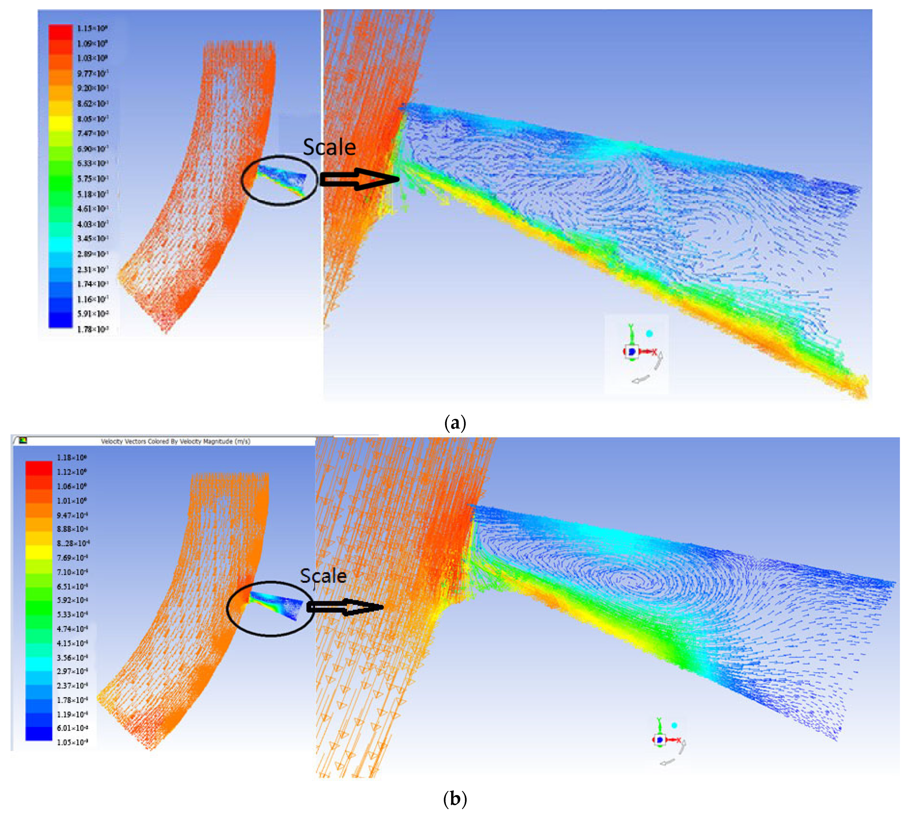
The fluid passing through the screen in the TPHS can be abstracted into a simple fan model. The flow rate and the driving force models of the permeating fluid were built using this model (see Equations (26) and (28) in Section 3.1). Furthermore, for the ideal fluid, the pressure difference near the screen aperture was the root cause of the penetration, which generated a higher radial velocity. The penetration process of the viscous fluid was affected not only by the pressure difference but also by the viscous force to produce a larger velocity gradient with a vortex. Under the same conditions, the sieving volume of the viscous fluid was greater than that of the ideal fluid.

(2)

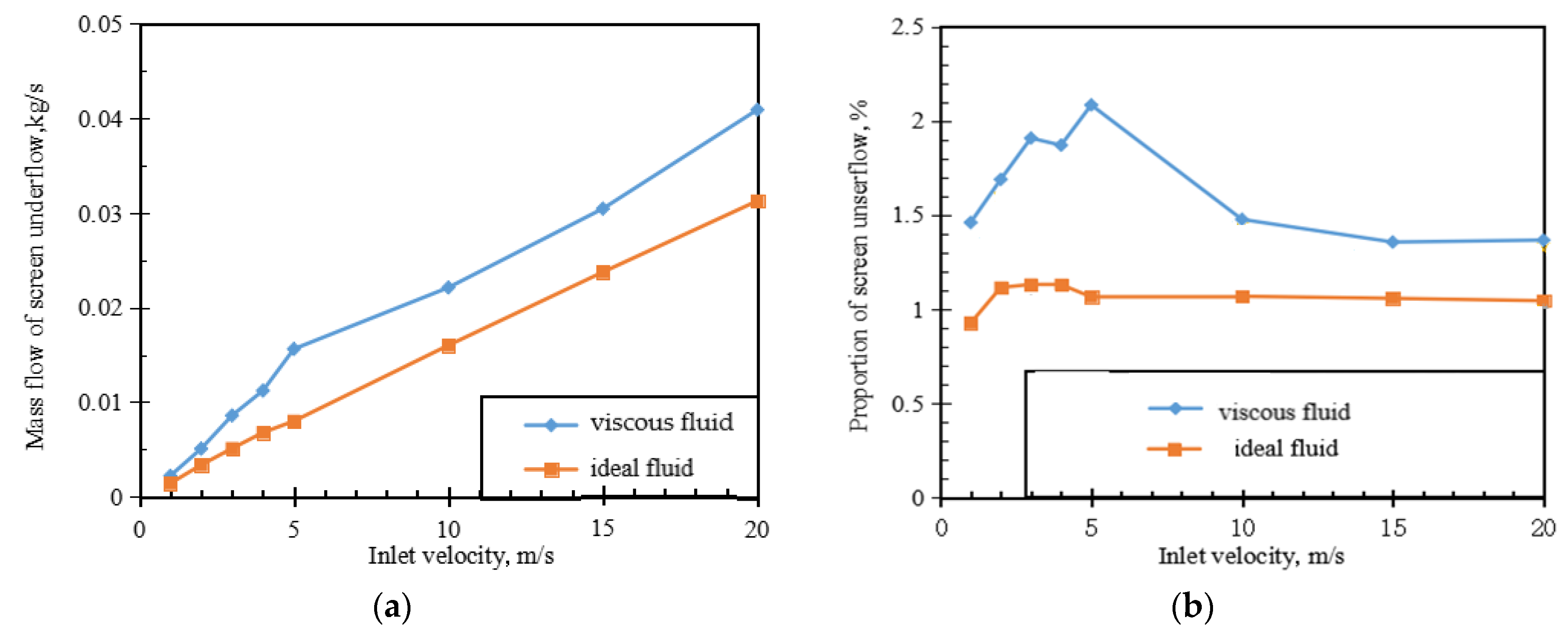
Under the same inlet velocity, the viscous fluid exhibited a higher flow rate than the ideal fluid during the permeating process. This demonstrates that the viscosity promoted the permeation. Furthermore, while the increased inlet velocity (0~20 m/s) increased the flow rate of the fluid passing through the screen, the proportion of the screen underflow first increased to a peak, then dropped, and then finally remained stable.

(3)

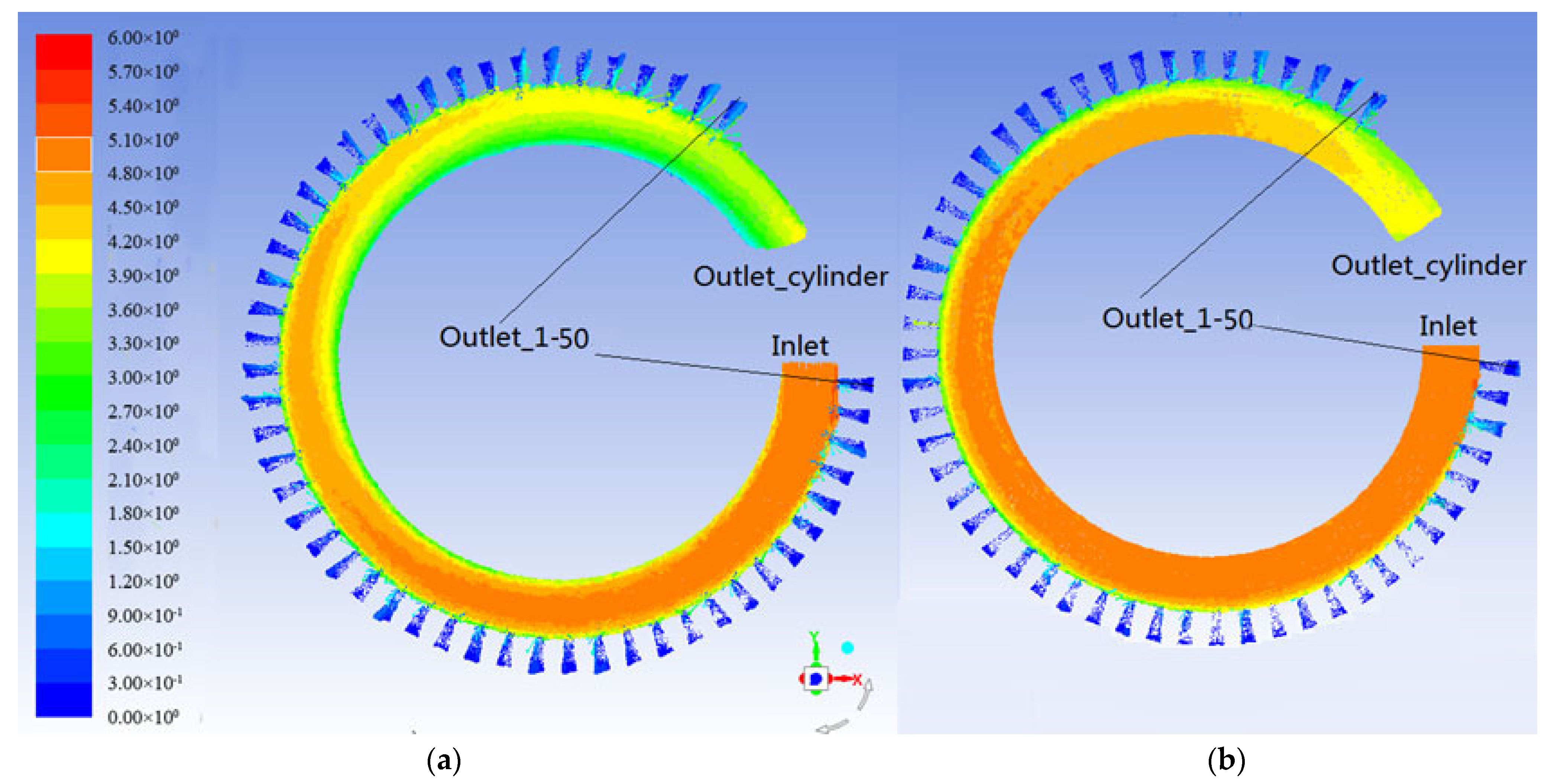
The CFD simulation results of the fluid permeation under the multiple screen aperture conditions were consistent with those of a single mesh. When there are multiple screen apertures in the direction of the fluid movement, the fluid permeability behaviour can be abstracted as the sum of the fluid permeability behaviour in each screen aperture. The fluid velocity gradually decreased along the flow direction at the same velocity inlet, and the viscous fluid decelerated faster than the ideal fluid. When compared to the ideal fluid, the viscous fluid had greater sieve penetration at the different screen apertures along the rotation direction.

(4)

The flow equation of the screen underflow for the TPHS was developed (see Equation (36) in Section 3.3), and it was related to the structure and the process parameters such as the rotation radius, length of the cylindrical screen, aperture size, open-area percentage, dynamic viscosity of the fluid, and pressure difference between the feed inlet and the screen outlet.

References

1. Wills, B.A.; Finch, J.A. (Eds.) Wills’ mineral processing technology: An introduction to the practical aspects of ore treatment and mineral recovery. In Wills’ Mineral Processing Technology, 8th ed.; Butterworth-Heinemann: Boston, MA, USA, 2016; pp. 1–27. [Google Scholar]
2. Eckert, K.; Schach, E.; Gerbeth, G.; Rudolph, M. Carrier Flotation: State of the Art and its Potential for the Separation of Fine and Ultrafine Mineral Particles. Mater. Sci. Forum 2019, 959, 125–133. [Google Scholar] [CrossRef]
3. Li, Z.; Fu, Y.; Yang, C.; Yu, W.; Liu, L.; Qu, J.; Zhao, W. Mineral liberation analysis on coal components separated using typical comminution methods. Miner. Eng. 2018, 126, 74–81. [Google Scholar] [CrossRef]
4. Obeng, D.P.; Morrell, S. The JK three-product cyclone—Performance and potential applications. Int. J. Miner. Process. 2003, 69, 129–142. [Google Scholar] [CrossRef]
5. Randjic, D. Proposition of new indices and parameters for grain size classification efficiency estimation. J. Min. Metall. A Min. 2008, 44, 17–23. [Google Scholar]
6. Honaker, R.Q.; Boaten, F.; Luttrell, G.H. Ultrafine coal classification using 150 mm gMax cyclone circuits. Miner. Eng. 2007, 20, 1218–1226. [Google Scholar] [CrossRef]
7. Wang, C.; Chen, J.; Shen, L.; Hoque, M.M.; Ge, L.; Evans, G.M. Inclusion of screening to remove fish-hook effect in the three products hydro-cyclone screen (TPHS). Miner. Eng. 2018, 122, 156–164. [Google Scholar] [CrossRef]
8. Chen, J.; Shen, L.; Wang, C.; Zhang, Y. Desliming performance of the three-product cyclone classification screen. Eng. Village 2016, 45, 813. [Google Scholar]
9. Wang, C.; Sun, X.; Shen, L.; Wang, G. Analysis and Prediction of Influencing Parameters on the Coal Classification Performance of a Novel Three Products Hydrocyclone Screen (TPHS) Based on Grey System Theory. Processes 2020, 8, 974. [Google Scholar] [CrossRef]
10. Yu, A.; Wang, C.; Liu, H.; Khan, M.S. Computational Modeling of Flow Characteristics in Three Products Hydrocyclone Screen. Processes 2021, 9, 1295. [Google Scholar] [CrossRef]
11. Davailles, A.; Climent, E.; Bourgeois, F. Fundamental understanding of swirling flow pattern in hydrocyclones. Sep. Purif. Technol. 2012, 92, 152–160. [Google Scholar] [CrossRef] [Green Version]
12. Wang, C.; Chen, J.; Shen, L.; Ge, L. Study of flow behaviour in a three products hydrocyclone screen: Numerical simulation and experimental validation. Physicochem. Probl. Miner. Process. 2019, 55, 879–895. [Google Scholar] [CrossRef]
13. Banerjee, C.; Chaudhury, K.; Majumder, A.K.; Chakraborty, S. Swirling Flow Hydrodynamics in Hydrocyclone. Ind. Eng. Chem. Res. 2015, 54, 522–528. [Google Scholar] [CrossRef]
14. Wang, C.; Yu, A.; Zhu, Z.; Liu, H.; Khan, M.S. Mechanism of the Absent Air Column in Three Products Hydrocyclone Screen (TPHS): Experiment and Simulation. Processes 2021, 9, 431. [Google Scholar] [CrossRef]
15. Xi-zeng, Z.; Chang-hong, H.; Zhao-chen, S. Numerical Simulation of Extreme Wave Generation Using VOF Method. J. Hydrodyn. 2010, 22, 466–477. [Google Scholar] [CrossRef]
16. Yuekan, Z.; Peikun, L.; Jiangbo, G.; Xinghua, Y.; Meng, Y.; Lanyue, J. Simulation analysis on the separation performance of spiral inlet hydrocyclone. Int. J. Coal Prep. Util. 2021, 41, 474–490. [Google Scholar]
17. Gibson, M.M.; Launder, B.E. Ground effects on pressure fluctuations in the atmospheric boundary layer. J. Fluid Mech. 1978, 86, 491–511. [Google Scholar] [CrossRef]
18. Leschziner, M.A.; Hogg, S. Computation of highly swirling confined flow with a Reynolds stress turbulence model. AIAA J. 1989, 27, 57–63. [Google Scholar] [CrossRef]
19. Yang, Z.; Cheng, X.; Zheng, X.; Chen, H. Reynolds-Averaged Navier-Stokes Equations Describing Turbulent Flow and Heat Transfer Behavior for Supercritical Fluid. J. Therm. Sci. 2021, 30, 191–200. [Google Scholar] [CrossRef]
20. StephenWhitaker. Flow in porous media I: A theoretical derivation of Darcy’s law. Transp. Porous Media 1986, 1, 3–25. [Google Scholar] [CrossRef]
21. Souza, F.J.; Vieira, L.G.M.; Damasceno, J.J.R. Analysis of the influence of the filtering medium on the behaviour of the filtering hydrocyclone. Powder Technol. 2000, 107, 259–267. [Google Scholar] [CrossRef]
22. Vieira, L.G.M.; Barbosa, E.A.; Damasceno, J.J.R.; Barrozo, M.A.S. Performance analysis and design of filtering hydrocyclones. Br. J. Chem. Eng. 2005, 22, 143–152. [Google Scholar] [CrossRef]
Figure 1. Diagram of 75 mm three products hydrocyclone screen (TPHS) (a) front view and (b) vertical view.
Processes 10 00628 g001
Figure 2. Fluid passing through single aperture (a) simple model and (b) cylindrical coordinate system.
Processes 10 00628 g002
Figure 3. Schematic diagram of the fluid passing through the screen in the cylindrical coordinate system (a) 2D plane flow and (b) scale.
Processes 10 00628 g003
Figure 4. Distribution of velocity vector (a) ideal and (b) viscous fluid.
Processes 10 00628 g004
Figure 5. Distribution of (a) the mass flow of screen underflow and (b) the proportion of screen underflow for ideal and viscous fluid under different inlet velocities (1~20 m/s).
Processes 10 00628 g005
Figure 6. Velocity vector with multi-apertures for (a) viscous and (b) ideal fluid with inlet velocity 1 m/s.
Processes 10 00628 g006
Figure 7. Distribution of the proportion of screen underflow under multi-aperture conditions.
Processes 10 00628 g007