A Novel Point-to-Point Trajectory Planning Algorithm for Industrial Robots Based on a Locally Asymmetrical Jerk Motion Profile

Abstract

Suitable trajectories with minimum execution time are essential for an industrial robot to enhance productivity in pick and place operations. A novel point-to-point trajectory planning algorithm (PTPA) is proposed to improve the motion efficiency of industrial robots. The jerk profile for a trajectory model is determined by five intervals and the jerk constraint. According to the kinematic constraints and two shape coefficients, a velocity threshold and three displacement thresholds are calculated for an individual joint to transfer the proposed jerk motion profile into four specific profiles. The optimal trajectory model of the joint is developed for the minimum-time and jerk-continuous trajectory via the performance evaluation with the input displacement and three displacement thresholds. Moreover, time-based motion synchronization for all joints is taken into account in PTPA to decrease unnecessary burdens on the actuators. The simulations illustrate that the execution time by PTPA is more efficient than that by other techniques. The experiments of a point-to-point application on a real six-axis industrial robot show that the absolute errors at the end of the motion for all joints are within 0.04°. These results prove that PTPA can be an effective point-to-point trajectory planner for industrial robots

1. Introduction

Industrial robots (IRs) have become one of the most important devices in the automotive, electronics, metal and other industries to replace the manual resource, due to their outstanding performances in terms of accuracy, repeatability and efficiency [1,2,3,4,5]. Trajectory planning for IRs, a fundamental issue in these automated industrial activities [6], generates reference inputs for the controller to implement certain tasks [7], such as pick and place operations [8], and assembly operations [9]. A pick and place operation, in essence, is a point-to-point (PTP) trajectory planning problem for a suitable and smooth trajectory from an initial position to a goal position. Otherwise, the possible excitation of mechanical resonance mode may result in noise and decrease of the lifetime of IRs [10,11].

In the literature, some research efforts have attempted to employ elementary functions for a smooth trajectory, including the polynomial, trigonometric, exponential function, etc. [12]. Jond et al. employed the polynomials of degrees 3, 4 and 5 to perform trajectory motions with continuous velocity and acceleration, where the acceleration values at the beginning and end motion are non-zero [13]. Boryga et al. planned the acceleration profile with the polynomials of degrees 5, 7 and 9 [14]. Fang et al. utilized the trigonometric function to build up a frequency central pattern generator (CPG) trajectory model for cyclic point-to-point tasks [15]. Third-order exponential function [16] and hyperbolic tangent function [17] were also adopted to generate smooth trajectories for PTP motions. These approaches result in jerk-continuous trajectories in the case of kinematic constraints, and the jerk values at the beginning and end movement are zero [14,15,16,17]. However, the trajectory based on the elementary functions causes low-efficiency motion of a robot due to no acceleration phase or constant velocity phase.

Substantial research has been focused on the composition of elementary functions to improve the motion efficiency of trajectory models. The quadrinomial polynomial was utilized to connect the initial point and intermediate point (a virtual knot), while the quintic polynomial was employed to link the intermediate point and final point [18,19,20]. Similarly, Bureerat et al. adopted the quintic polynomial to connect the initial point and intermediate point (a virtual knot) and then to the final point [21]. Other trajectory models based on polynomial compositions have also been utilized to generate smooth PTP trajectories, such as cubic spline [22], fifth-order B-spline [23], trapezoidal velocity profile [24] and polynomial S-curve models (i.e., motion profiles) [25,26,27,28]. In addition, Perumaal and Jawahar employed a trigonometric S-curve model with a polynomial of degree 2 to generate jerk-bound trajectories with synchronized acceleration, constant velocity and deceleration phases [29]. Motived by their work, Valente et al. adopted the generated trajectories with asynchronous acceleration and deceleration phases, and found they greatly extended the number of feasible solutions [30]. To better utilize the kinematic constraints, one or both of the constant acceleration and jerk phases was added to the motion profiles for trajectory models [31,32,33]. Among these models, the trajectory model based on a sinusoidal jerk motion profile with fifteen segments has shown its superiority in motion efficiency for pick and place operations [31]. Nevertheless, the trajectory resulting from the jerk profile with a high ramp coefficient leads to the low-efficiency motion of a robot due to the similar ramp-up to the ramp-down in the jerk profile.

Some researchers also paid abundant attention to pursuing optimal solutions based on various objectives, such as minimum-time [14,15,16,30,31,32,33], minimum-jerk [21,22,23], minimum-energy [34,35], etc. The numerical and analysis methods are two optimal solutions for the solver type. Valente et al. adopted an active-set algorithm to globally minimize the total motion time [30]. Chettibi et al. employed the sequential quadratic programming (SQP) method to obtain the minimum cost with transfer time and the quadratic average of both actuator efforts and corresponding power [22]. Intelligent algorithms, such as genetic algorithm (GA) [13,18,19], artificial bee colony (ABC) algorithm [20] and differential evolution (DE) algorithm [21] can solve the multi-objective optimization problems for trajectory planning. The numerical method may fail to obtain a solution or become trapped in local convergence, due to the unsuitable selection of an initial solution and high computational complexity. Then, some studies are focused on the closed-form solutions for the global minimum and high computational efficiency by using the kinematic constraints. The properties of root multiplicity were employed to generate the high-order polynomial trajectory model by only one polynomial coefficient which can be computed from the kinematic limits [14,27]. The execution time can be minimized from the kinematic limits and input displacements [15,16,25,31,32,33].

The goal of this work is to provide a closed-form solution for the time-optimal and smooth trajectory planning of IRs based on an improved jerk motion profile. Since the motion with high efficiency for a robot can be produced by the kinematic peak values of a trajectory model, the locally asymmetrical jerk motion profile with low jerk ramp-up is proposed for the trajectory model to obtain rapidly the jerk peak value. The ramp coefficient and local asymmetry coefficient are adopted to reduce the number of determined intervals for the jerk profile. Furthermore, the relationship between the execution time and the two shape coefficients is investigated quantitatively to improve the motion efficiency with lower jerk ramp-up. According to the two coefficients and the kinematic constraints, four thresholds are calculated for an individual joint to transfer the proposed jerk motion profile into four specific profiles. Then, the optimal trajectory model of the joint is ascertained for the minimum-time and jerk-continuous trajectory via the performance evaluation with the input displacement and three displacement thresholds. Moreover, time-based motion synchronization for all joints is also taken into account in the proposed algorithm to decrease unnecessary burdens on the actuators.

The structure of this paper is organized as follows. Section 2 introduces the proposed trajectory model based on a locally asymmetrical sine jerk profile and spreads out the corresponding mathematical formulas. This section also presents the impact of two shape coefficients on the execution time. Section 3 presents a formal definition of the time-optimal trajectory planning problem. PTPA is proposed in Section 4. Section 5 presents the simulation results compared with other methods and experimental results on a real industrial robot. Concluding remarks and future extensions are given in Section 6.

2. Proposed Trajectory Model

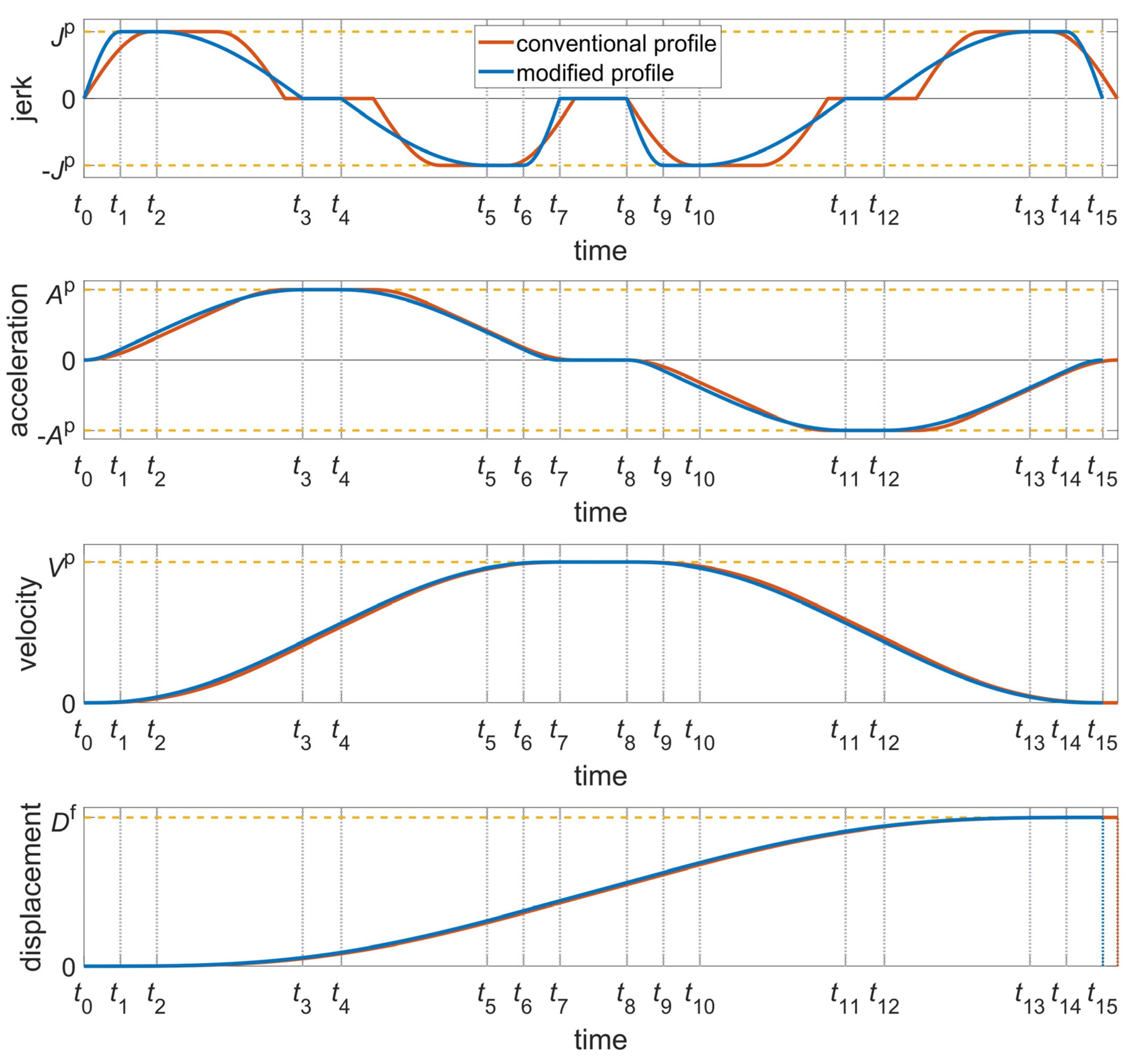
2.1. Locally Asymmetrical Jerk Motion Profile

The conventional trajectory model with constant acceleration and velocity phases has similar ramp-up and ramp-down segments in the jerk motion profile (red line in Figure 1), which may reduce the motion efficiency in the case of a high ramp coefficient [31]. Thus, to overcome this deficiency, we propose the locally asymmetrical jerk motion profile with low ramp-up, as shown (blue line in Figure 1). We define the terms similarly in [36] to describe the trajectory segments. D^f denotes the displacement at the end of the sustained pulse of the velocity. V^p, A^p and J^p represent the peak values of the velocity, acceleration and jerk during the motion, respectively. t_i represents the time at the end of the ith segment, where i ∈ {0, 1, …, 15}.

The trajectory model comprises three phases: the acceleration phase (AP) when t ∈ [t₀, t₇], the constant velocity phase (CVP) when t ∈ [t₇, t₈], and the deceleration phase (DP) when t ∈ [t₈, t₁₅]. Let T_i denote the interval of the ith segment, i.e., T_i = t_i-t_i−1, where i ∈ {1, …, 15}. We assume that T₁ = T₇ = T₉ = T₁₅, T₂ = T₆ = T₁₀ = T₁₄, T₃ = T₅ = T₁₁ = T₁₃ and T₄ = T₁₂. Then, as shown in Figure 1, the ramp-up and ramp-down of the velocity and acceleration are all symmetrical all the time. Note that a locally asymmetrical jerk motion profile exists in the case of T₁ ≠ T₃. Then, the execution time T_t can be expressed as

$$T_{\mathrm{t}}=4T_1+4T_2+4T_3+2T_4+T_8.$$

(1)

where T₁, T₂ and T₃ are the intervals of the ramp-up, cruise and ramp-down of the jerk, respectively; T₄ and T₈ are the intervals of the acceleration cruise and the velocity cruise, respectively. The locally asymmetrical jerk motion profile in Figure 1 is defined as

$$J(t)=sign(D^{\mathrm{f}})\left\{\begin{array}{cc}\hfill J^{\mathrm{p}}\sin (\frac{\mathsf{\pi }(t-t_{i-1})}{2T_i}),& i=1,13\hfill \\ \hfill J^{\mathrm{p}},& i=2,14\hfill \\ \hfill J^{\mathrm{p}}\sin (\frac{\mathsf{\pi }}{2}+\frac{\mathsf{\pi }(t-t_{i-1})}{2T_i}),& i=3,15\hfill \\ \hfill 0,& i=4,8,12\hfill \\ \hfill -J^{\mathrm{p}}\sin (\frac{\mathsf{\pi }(t-t_{i-1})}{2T_i}),& i=5,9\hfill \\ \hfill -J^{\mathrm{p}},& i=6,10\hfill \\ \hfill -J^{\mathrm{p}}\sin (\frac{\mathsf{\pi }}{2}+\frac{\mathsf{\pi }(t-t_{i-1})}{2T_i}),& i=7,11\hfill \end{array}\right..$$

(2)

Let A_i, V_i and D_i denote the motion profiles of the acceleration, velocity and displacement for the ith segment, respectively. Given the initial conditions of the ith segment, A_i, V_i and D_i can be computed by sequentially integrating their corresponding jerk equations, and are given by

$$\left\{\begin{array}{l}{A}_i(t)=A_{i-1}^{\mathrm{e}}+{\displaystyle {\int }_{t_{i-1}}^{t}J(t)dt}\\ V_i(t)=V_{i-1}^{\mathrm{e}}+{\displaystyle {\int }_{t_{i-1}}^t{A}_i(t)dt}\\ D_i(t)=D_{i-1}^{\mathrm{e}}+{\displaystyle {\int }_{t_{i-1}}^t{V}_i(t)dt}\end{array}\right..$$

(3)

where A_i−1^e, V_i−1^e and D_i−1^e (i = 1, 2, …, 15) denote the values of the acceleration, velocity and displacement at the end of the (i−1)th segment, respectively. For example, A₀^e, V₀^e and D₀^e, represent the initial conditions of the acceleration, velocity and displacement of the first segment, respectively. The symmetry of the proposed jerk profile can simplify the integration process. The detailed equations of each segment are expressed in the Appendix A. Here, several important equations are utilized to compute the determined intervals. A^p and V₃^e are the acceleration and velocity reached at the end of the first acceleration ramp-up from zero acceleration to A^p, respectively, and are given by

$$A^{\mathrm{p}}=A_3^{\mathrm{e}}=J^{\mathrm{p}}\left(\frac{2T_3}{\mathsf{\pi }}+T_2+\frac{2T_1}{\mathsf{\pi }}\right),$$

(4)

$$V_3^{\mathrm{e}}=J^{\mathrm{p}}\left(\frac{2^2}{{\mathsf{\pi }}^2}{T}_3^2+T_2{T}_3+\frac{2}{\mathsf{\pi }}{T}_1{T}_3+\frac{1}{2}{T}_2^2+\frac{2}{\mathsf{\pi }}{T}_1{T}_2+(\frac{2}{\mathsf{\pi }}-\frac{2^2}{{\mathsf{\pi }}^2})T_1^2\right).$$

(5)

V^p and D₇^e are the velocity and displacement reached at the end of the velocity ramp-up from zero speed to V^p, respectively, and are described as

$$V^{\mathrm{p}}=V_7^{\mathrm{e}}=2V_3^{\mathrm{e}}+A^{\mathrm{p}}{T}_4,$$

(6)

$$D_7^{\mathrm{e}}=J^{\mathrm{P}}\left(\begin{array}{l}(-\frac{8}{{\mathsf{\pi }}^2}+\frac{4}{\mathsf{\pi }})T_1^3+(\frac{4}{\mathsf{\pi }}-\frac{4}{{\mathsf{\pi }}^2})T_1^2{T}_4+(\frac{8}{\mathsf{\pi }}-\frac{8}{{\mathsf{\pi }}^2})T_1^2{T}_3+(\frac{8}{\mathsf{\pi }}-\frac{8}{{\mathsf{\pi }}^2})T_1^2{T}_2\\ +\frac{1}{\mathsf{\pi }}{T}_1{T}_4^2+(\frac{8}{{\mathsf{\pi }}^2}+\frac{4}{\mathsf{\pi }})T_1{T}_3^2+(1+\frac{4}{\mathsf{\pi }})T_1{T}_2^2+\frac{6}{\mathsf{\pi }}{T}_1{T}_3{T}_4+(1+\frac{4}{\mathsf{\pi }})T_1{T}_2{T}_4\\ +(2+\frac{8}{\mathsf{\pi }})T_1{T}_2{T}_3+T_2^3+\frac{3}{2}{T}_2^2{T}_4+3T_2^{2}T+\frac{1}{2}{T}_2{T}_4^2+(2+\frac{8}{{\mathsf{\pi }}^2})T_2{T}_3^2\\ +(2+\frac{2}{\mathsf{\pi }})T_2{T}_3{T}_4+\frac{8}{{\mathsf{\pi }}^2}{T}_3^3+(\frac{2}{\mathsf{\pi }}+\frac{4}{{\mathsf{\pi }}^2})T_3^2{T}_4+\frac{1}{\mathsf{\pi }}{T}_3{T}_4^2\end{array}\right).$$

(7)

D^f is the displacement reached at the end of the movement and is given by

$$D^{\mathrm{f}}=D_{15}^{\mathrm{e}}=2D_7^{\mathrm{e}}+V_7^{\mathrm{e}}{T}_8.$$

(8)

If J^p is specified, the proposed trajectory model can be fully determined by the five intervals T₁, T₂, T₃, T₄ and T₈. However, the number of the determined intervals is still too many to form a closed-form solution for a time-optimal trajectory.

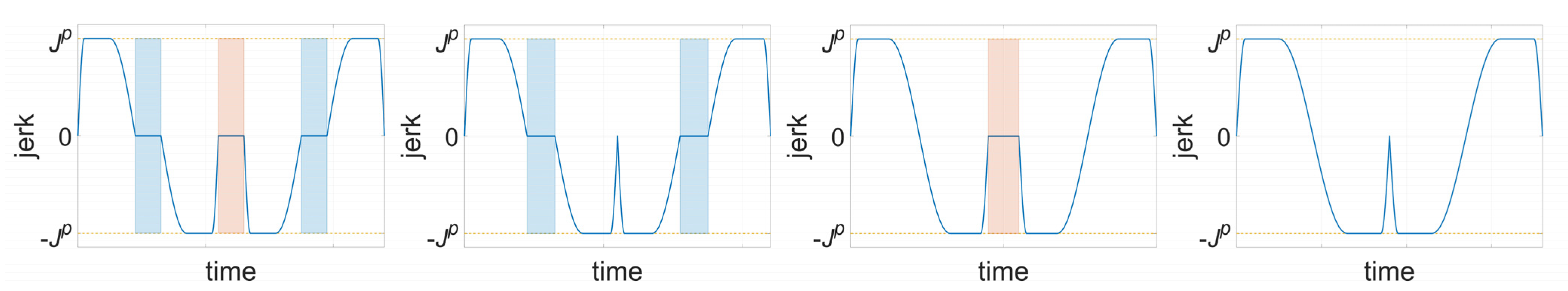
2.2. Shape Coefficients

To decrease the number of the determined intervals and enhance the computational efficiency, the relationships between T₁ and T₂, T₁ and T₃ are established, respectively. T₄ and T₈ are both set to zero in this subsection, because they may not exist in some circumstances, e.g., a case with large kinematic limits and low displacement. Moreover, to avoid the impact of the constraints on the execution time, we assume that the kinematics limits cannot be reached. Then, two shape coefficients are adopted to describe the shape of the jerk profile. Let α and β denote the ramp coefficient and the local asymmetry coefficient, respectively, which are expressed as

$$\alpha =\frac{T_1}{T_1+T_2},$$

(9)

$$\beta =\frac{T_1}{T_1+T_3}.$$

(10)

Nonzero jerk can occur at the initial and goal positions during the motion when α or β is set to 0 (i.e., T₁ = 0), which will increase the wear of the robot structure and should be avoided to enhance the reliability of IRs. Thus, α > 0 and β > 0, i.e., T₁ > 0. In addition, to generate a jerk-continuous trajectory, β ≠ 1 (i.e., T₃ ≠ 0). Note that the local jerk profile is symmetrical when β = 0.5 (i.e., T₁ = T₃). Therefore, the domain of α is set to (0, 1] and β to (0, 1), to ensure that the jerk of the generated trajectory is continuous and its values are zero at the initial and goal positions. The jerk motion profiles with different α and β are shown in Figure 2.

As T₄ = 0 and T₈ = 0, substituting Equations (8)–(10) into Equation (1), T_t is related to α and β by

$$T_{\mathrm{t}}=4\sqrt[3]{\frac{D^{\mathrm{f}}}{J^{\mathrm{p}}}}\left(\frac{\alpha +\beta -\alpha \beta }{\alpha \beta }\right)\sqrt[3]{\frac{1}{c_1}},$$

(11)

where

$$c_1=2\left(\begin{array}{l}(-\frac{8}{{\mathsf{\pi }}^2}+\frac{4}{\mathsf{\pi }})T_1^3+(\frac{8}{\mathsf{\pi }}-\frac{8}{{\mathsf{\pi }}^2})\frac{1-\beta }{\beta }+(\frac{8}{\mathsf{\pi }}-\frac{8}{{\mathsf{\pi }}^2})\frac{1-\alpha }{\alpha }+(\frac{8}{{\mathsf{\pi }}^2}+\frac{4}{\mathsf{\pi }}){(\frac{1-\beta }{\beta })}^2\\ +(1+\frac{4}{\mathsf{\pi }}){(\frac{1-\alpha }{\alpha })}^2+(2+\frac{8}{\mathsf{\pi }})\frac{1-\alpha }{\alpha }\frac{1-\beta }{\beta }+{(\frac{1-\alpha }{\alpha })}^3+3{(\frac{1-\alpha }{\alpha })}^2\frac{1-\beta }{\beta }\\ +(2+\frac{8}{{\mathsf{\pi }}^2})\frac{1-\alpha }{\alpha }{(\frac{1-\beta }{\beta })}^2+\frac{8}{{\mathsf{\pi }}^2}{(\frac{1-\beta }{\beta })}^3\end{array}\right).$$

(12)

Thus, D^f and J^p can be considered as the proportionality coefficients of T_t, and the variation trend of T_t is only determined by α and β. For example, when D^f = 140 deg and J^p = 70 rad/s³, the impact of different α and β on T_t is depicted in Figure 3.

In Figure 3, T_t declines significantly and steadily with the decreasing β when α ≥ 0.5. The reason is that the jerk can rapidly reach the peak as T₁ decreases with smaller β. However, the impact is different when α < 0.5. There exists a threshold with the smallest execution time T_t. Let β_th denote the threshold. β_th increases with the decreasing α, and approaches 0.5 when α is fairly close to 0, because the jerk profile considerably approaches the bang-bang jerk profile. Therefore, for a given α, there is a corresponding β with the smallest execution time.

3. Optimal Problem Formulation

The optimal 14 of PTP trajectory planning for IRs is generally presented in the Cartesian space or the joint space. Planning trajectory in the joint space is difficult to predict the motion of the end effector of IRs, but it can avoid kinematic singularities and reduce the computational complexity, compared with that in the Cartesian space [37]. Therefore, the goal of this paper is to obtain time-optimal trajectories in the joint space.

Let ℕ_>0 be the set of positive integers and ℝ the set of reals. Let ℝ_≥0, ℝ_>0 and ℝ_<0 represent the sets of non-negative, positive and negative reals, respectively. Then, let n ∈ ℕ_>0 be the number of the joints of an industrial robot. Clearly, |V^p|, A^p, J^p, T_t ∈ ℝ_>0ⁿ. Let m ∈ ℕ_>0 denote the number of the trajectory segments. Then, let Γ ∈ ℝ_≥0^m×n denote the matrix of the interval, i.e., Γ = {T_i,g}, where i, g ∈ ℕ_>0, i ≤ m and g ≤ n. The 1-norm is denoted by ||·||₁. Note that ||Γ||₁ = max {T_t}. Thus, the objective function in this paper can be described as

τ = min{||Γ||₁}.

(13)

Let V^max, A^max, J^max ∈ ℝ_>0ⁿ denote the kinematic limits of the velocity, acceleration and jerk of an industrial robot, respectively. We assume that V^min = −V^max, A^min = −A^max and J^min = −J^max, where V^min, A^min, J^min ∈ ℝ_<0ⁿ are the constraint minimum of the velocity, acceleration and jerk, respectively. Then, the kinematic constraints of the optimality problem are given by

$$\left\{\begin{array}{c}\left|V^{\mathrm{p}}\right|\le V^{\max }\\ A^{\mathrm{p}}\le A^{\max }\\ J^{\mathrm{p}}\le J^{\max }\end{array}\right..$$

(14)

Let θ_initial, θ_goal ∈ ℝⁿ denote the initial and goal positions, respectively. Given a, b ∈ ℝ, a closed interval between a and b is denoted by [a, b]. Consequently, the optimality problem of the PTP trajectory planning in this paper is to find feasible trajectories with minimal objective function while respecting the kinematic constraints, formalized as follows.

Given an initial position θ_initial, a goal position θ_goal, and the kinematic limits of the velocity V^max, acceleration A^max and jerk J^max, find trajectories Ω: [0, τ] → ℝⁿ such that (i) Ω(0) = θ_initial and Ω(τ) = θ_goal, (ii) τ = min{||Γ||₁}, and (iii) |V^p| ≤ V^max, A^p ≤ A^max and J^p ≤ J^max.

4. Point-to-Point Trajectory Planning Algorithm

A PTPA is proposed to provide a closed-form solution for the time-optimal PTP trajectory. PTPA is divided into four procedures: data input, initialization, minimum-time calculation and motion synchronization. Pseudo-code of PTPA is shown in Algorithm 1.

Algorithm 1: PTPA

Input:θinitial, θgoal, Vmax, Amax, Jmax, α and β

Output:Ω

Start

Generate the displacements Df = θgoal − θinitial

Compute the thresholds Vamax, Damax, Dvmax1, Dvmax2 using Equations (18), (19), (23) and (26)

forg = 1 to n do

ifVgamax < Vgmax

if Dgf > Dgvmax1

Compute T1,g, T2,g, T3,g, T4, g and T8,g according to Type I

else if Dgamax < Dgf ≤ Dgvmax1

T8,g = 0

Compute T1,g, T2,g, T3,g and T4,g according to Type II

end if

else ifDgf > Dgvmax2

T4,g = 0

Compute T1,g, T2,g, T3,g and T8,g according to Type III

else

T4,g = 0, T8,g = 0

Compute T1,g, T2,g and T3,g according to Type IV

end if

end for

Generate the execution time τ using Equation (28)

Compute the scaling coefficient k using Equation (29)

Synchronize the motion profiles of each joint trajectory

end

4.1. Minimum Time

According to T₄ and T₈, the jerk motion profiles are classified into four specific ones to improve the computational efficiency, as shown in Figure 4. For a given PTP task of an industrial robot, the type of jerk motion profile of a joint is mainly determined by a velocity threshold, three displacement thresholds and an input displacement. Let V_g^amax ∈ ℝ be the velocity threshold, and D_g^amax, D_g^vmax1, D_g^vmax2 ∈ ℝ the three displacement thresholds. Note that the subscript g refers to the gth joint.

V_g^amax: the velocity reached at the end of the acceleration pulse from zero acceleration to A_g^max and back down to zero acceleration, without taking the velocity limit into account.

D_g^amax: the displacement reached at the end of the velocity pulse from zero velocity to V_g^amax and back down to zero velocity (i.e., V_g^p = V_g^amax).

D_g^vmax1: the displacement reached at the end of the velocity pulse from zero velocity to V_g^max and back down to zero velocity (i.e., V_g^p = V_g^max), while V_g^amax is smaller than V_g^max (i.e., V_g^amax < V_g^max = V_g^p).

D_g^vmax2: the displacement reached at the end of the velocity pulse from zero velocity to V_g^max and back down zero velocity (i.e., V_g^p = V_g^max), while V_g^max is smaller than or equal to V_g^amax (i.e., V_g^p = V_g^max ≤ V_g^amax).

The shortest execution time can be achieved by utilizing the kinematic limits [14,15,16,31,32,33]. However, the velocity and acceleration limits may be unavailable in some tasks, such as a small displacement with large kinematic limits. Therefore, we assume that J^p = J^max in this part. Note that only the definitions of T_1,g, T_4,g and T_8,g are given, since T_2,g and T_3,g can be obtained from T_1,g by using Equations (9)–(10) if α and β are specified.

Type I: T_4,g > 0, T_8,g > 0.

T_4,g >0 implies that the acceleration limit A_g^max must be reached at the end of the first acceleration ramp-up (i.e., A_g^p = A_g^max), and V_g^amax must be smaller than V_g^p (i.e., V_g^p > V_g^amax). Thus, T_1,g is obtained by substituting Equations (9) and (10) into Equation (4):

$$T_{1,g}=\frac{A_g^{\max }\mathsf{\pi }\alpha \beta }{J_g^{\max }(2\alpha +\mathsf{\pi }\beta -\mathsf{\pi }\alpha \beta )}.$$

(15)

T_8,g > 0 represents that the velocity limit V_g^max must be reached at the end of the velocity ramp-up (i.e., V_g^p = V_g^max). Then, T_4,g is obtained by using Equation (6):

$$T_{4,g}=\frac{V_g^{\max }-2V_{3,g}^{\mathrm{e}}}{A_g^{\max }}.$$

(16)

Furthermore, the displacement D_g^f must be greater than D_g^vmax1 (i.e., D_g^f > D_g^vmax1). Then, T_8,g is obtained by using Equation (8):

$$T_{8,g}=\frac{D_g^{\mathrm{f}}-2D_{7,g}^{\mathrm{e}}}{V_g^{\max }}.$$

(17)

Consequently, this type can be selected when V_g^max > V_g^amax and D_g^f > D_g^vmax1. Then, V_g^amax can be obtained by using Equation (6) when T_4,g = 0:

$$V_g^{\mathrm{amax}}=2V_{3,g}^{\mathrm{e}}.$$

(18)

Moreover, D_g^vmax1 can be obtained by using Equation (8) when T_8,g = 0:

$$D_g^{\mathrm{vmax}1}=2D_{7,g}^{\mathrm{e}}.$$

(19)

Type II: T_4,g > 0, T_8,g = 0.

In this type, T_1,g can be obtained in the same way that in type I, since T_4,g > 0. T_8,g = 0 means that the displacement D_g^f must be equal to or smaller than D_g^vmax1 (i.e., D_g^f ≤ D_g^vmax1). Additionally, D_g^f also must be greater than D_g^amax (i.e., D_g^f > D_g^amax), since T_4,g must be equal to 0 if D_g^f is equal to or smaller than D_g^amax. Then, substituting Equations (6), (9) and (10) into Equation (7), T_4,g can be computed by:

$$T_{4,g}=\frac{-c_3\pm \sqrt{{(c_3)}^2-4c_2\left(c_1-\frac{D_g^{\mathrm{f}}}{2J_g^{\max }{(T_{1,g})}^3}\right)}}{2c_2}{T}_{1,g},$$

(20)

where

$$c_2=\frac{1}{\mathsf{\pi }}+\frac{1-\beta }{\mathsf{\pi }\beta }+\frac{1-\alpha }{2\alpha },$$

(21)

$$c_3=\left\{\begin{array}{l}(\frac{4}{\mathsf{\pi }}-\frac{4}{{\mathsf{\pi }}^2})+\frac{3}{2}{(\frac{1-\alpha }{\alpha })}^2+(\frac{2}{\mathsf{\pi }}+\frac{4}{{\mathsf{\pi }}^2}){(\frac{1-\beta }{\beta })}^2\\ +\frac{6}{\mathsf{\pi }}\frac{1-\beta }{\beta }+(1+\frac{4}{\mathsf{\pi }})\frac{1-\alpha }{\alpha }+(2+\frac{2}{\mathsf{\pi }})\frac{1-\alpha }{\alpha }\frac{1-\beta }{\beta }\end{array}\right..$$

(22)

Consequently, this type can be selected when V_g^max > V_g^amax and D_g^amax < D_g^f ≤ D_g^vmax1. Then, D_g^amax can be obtained by substituting Equations (6), (9), (10) and (15) into Equation (7) when T_4,g = 0:

$$D_g^{\mathrm{amax}}=\frac{c_1{(A_g^{\max }\mathsf{\pi }\alpha \beta )}^3}{{(J_g^{\max })}^2{(2\alpha +\mathsf{\pi }\beta -\mathsf{\pi }\alpha \beta )}^3}.$$

(23)

Type III: T_4,g = 0, T_8,g > 0.

T_4,g = 0 implies that V_g^p must be equal to or smaller than V_g^amax (i.e., V_g^p ≤ V_g^amax). T_8,g > 0 represents that V_g^p = V_g^max as mentioned previously. Additionally, the displacement D_g^f must be greater than D_g^vmax2 (i.e., D_g^f > D_g^vmax2). Consequently, this type can be selected when V_g^max ≤ V_g^amax and D_g^f > D_g^vmax2. Note that T_8,g can be computed from Equation (17), if T_1,g is given.

Substituting Equations (4), (9) and (10) into Equation (5), T_1,g can be computed by:

$$T_{1,g}=\sqrt{\frac{V_g^{\max }}{J_g^{\max }{c}_4}},$$

(24)

where

$$c_4=2\left(\frac{2^2{(1-\beta )}^2}{{\mathsf{\pi }}^2{\beta }^2}+\frac{(1-\alpha )(1-\beta )}{\alpha \beta }+\frac{2(1-\beta )}{\mathsf{\pi }\beta }+\frac{{(1-\alpha )}^2}{2{\alpha }^2}+\frac{2(1-\alpha )}{\mathsf{\pi }\alpha }+(\frac{2}{\mathsf{\pi }}-\frac{2^2}{{\mathsf{\pi }}^2})\right).$$

(25)

D_g^vmax2 can be obtained by substituting Equations (6), (9), (10) and (24) into Equation (7):

$$D_g^{\mathrm{vmax}2}=c_1\sqrt{\frac{{(V_g^{\max })}^3}{J_g^{\max }{(c_5)}^3}}.$$

(26)

Type IV: T_4,g = 0, T_8,g = 0.

Except for the three types above, T_1,g can be obtained by substituting Equations (6), (9) and (10) into Equation (7):

$$T_{1,g}=\sqrt[3]{\frac{D^{\mathrm{f}}}{J_g^{\max }{c}_1}}.$$

(27)

Four thresholds can be obtained, when α and β are specified for an industrial robot. Then, the jerk motion profile for the time-optimal trajectory model can be transferred into a specific one by comparing the input displacement and three displacement thresholds in a given PTP task. Thus, we can obtain the matrix of the interval Γ and the execution time T_t generated based on the specific profile.

4.2. Synchronization of Motion Profiles

Since the task and the kinematic limits are different for each joint of an industrial robot, their execution time varies in lengths. This may result in unnecessary burdens on the actuators without the synchronization of all joints. Time-based synchronization is taken into account to decrease the burden and ensure that all joints can start and stop at the designated position simultaneously. Due to the utilization of the kinematic limits, T_t can be considered as the minimum set of the execution time for each joint, such that

τ = {||Γ||₁} = max{T_t}.

(28)

Let k ∈ ℝ_>0ⁿ denote the set of the synchronization coefficients, i.e., k = {k_g}, where g ∈ ℕ_>0, g ≤ n,

$$k_g=\frac{\tau }{T_{\mathrm{t},g}}.$$

(29)

Let t ⸦ ℝ_≥0 denote the time variable, and D_g(k_gt), V_g(k_gt), A_g(k_gt), J_g(k_gt) ⸦ ℝⁿ the trajectory and its derivatives. Then, the following holds:

$$\left\{\begin{array}{c}{D}_g(k_{g}t)=D_g(t)\\ V_g(k_{g}t)=\frac{V_g(t)}{k_g}\\ A_g(k_{g}t)=\frac{A_g(t)}{{(k_g)}^2}\\ J_g(k_{g}t)=\frac{J_g(t)}{{(k_g)}^3}\end{array}\right..$$

(30)

For the joints with k_g > 1 in a given PTP task, the peak values of the velocity, acceleration and jerk decrease after synchronization, which can protect the drivers in the joints to extend their service life.

Herein, we summarized the procedures of PTPA. The initial and goal positions of each joint with their kinematic limits are defined in advance, as well as two shape coefficients. According to the kinematic constraints and the shape coefficients, the displacements and the thresholds are computed as the selection criterion for the jerk profile. A specific jerk profile of the optimal trajectory model for a joint is ascertained for the minimum-time and jerk-continuous trajectory via the performance evaluation with the input displacement and three displacement thresholds. Finally, the time-based motion synchronization for all joints is carried out to decrease unnecessary burdens on the actuators.

5. Results

To demonstrate the feasibility of the proposed algorithm, the numerical simulation and experiments tested on a real industrial robot were carried out. We ran the numerical simulations using the MATLAB R2018b on a Windows 10 personal computer with a Core i5-1035G1 CPU and 16 GB of RAM. An experimental platform was built up to mimic a pick and place operation, and validate the numerical simulations. This platform mainly included a six-axis industrial robot Universal Robots UR5, a robot controller CB3 and a personal computer with Linux operating system, as shown in Figure 5. The robot controller was controlled over TCP/IP protocol by a script implemented in Python using the Real-Time Data Exchange (RTDE) interface ur-rtde 1.4.3. The script fed the joint position targets to the robot controller to simulate a pick and place operation. This script was implemented on a personal computer with a Core-i3 4130 processor and 4 GB of RAM.

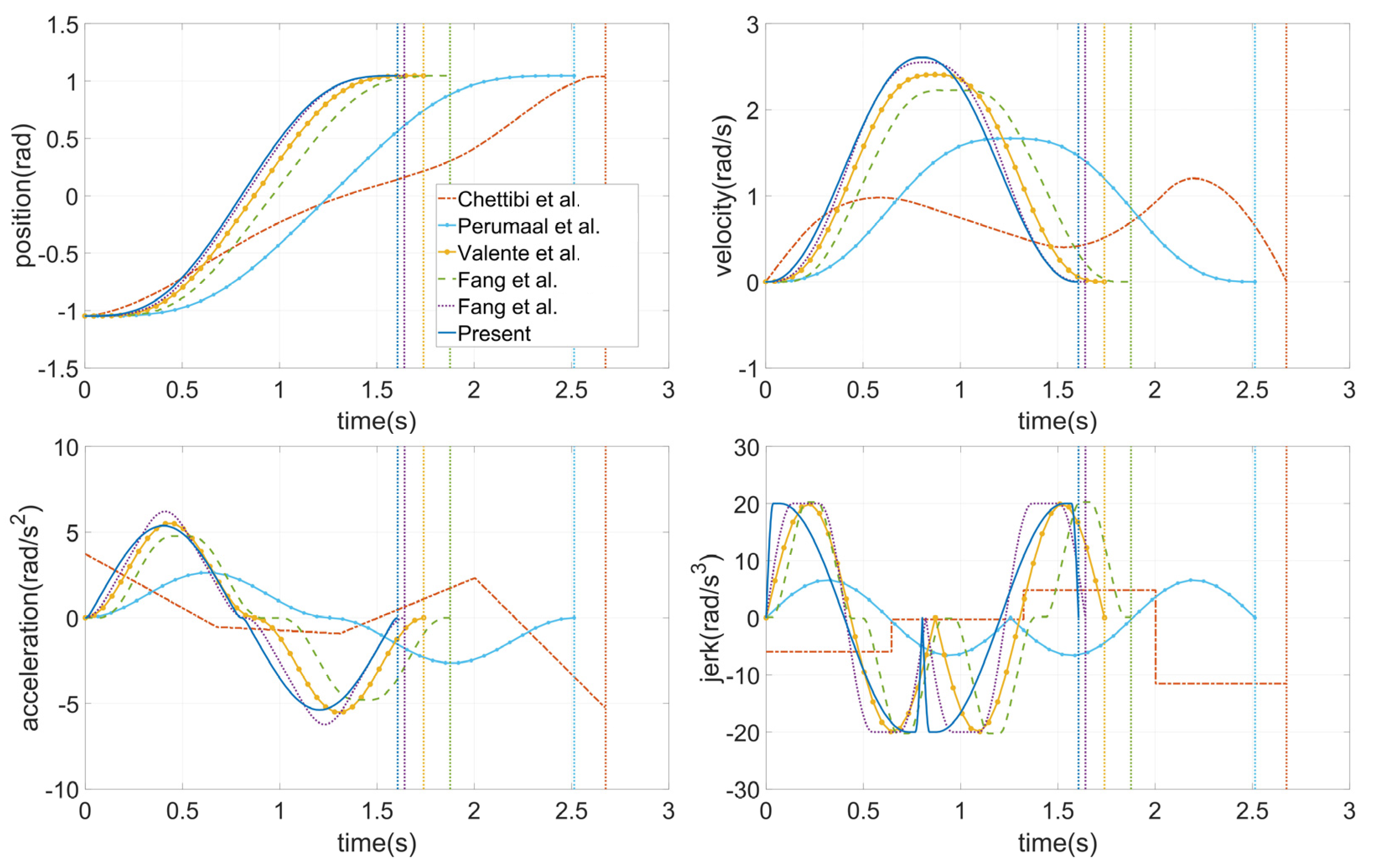
5.1. Numerical Simulation

A typical PTP task for a six-axis industrial robot was chosen to compare the simulated execution time by five different types of trajectories [22,29,30,31,32]. The PTP task to be tested is listed in

Table 1. Desired positions and kinematic limits of the test task.

		Joint No.
		1	2	3	4	5	6
Position	Initial position (rad)	0	−π/6	0	−π/3	0	0
	Goal position (rad)	2π/3	π/6	π/4	π/3	−π/4	π/6
Kinematic limits	Velocity (rad/s)	8	10	10	5	5	5
	Acceleration (rad/s2)	10	12	12	8	8	8
	Jerk (rad/s3)	30	40	40	20	20	20

, where the initial and goal positions of each joint are presented, as well as the kinematic limits of the velocity, acceleration and jerk. α was set to 0.1, 0.5 and 1 [31]. β was set to 0.3, 0.1 and 0.1 according to the Equations (11) and (12).

The motion profiles of joint 4 which determined the execution time, generated by the benchmark methods and this work, are shown in Figure 6. The cubic polynomial trajectory model failed to produce jerk-continuous motion, and the values of the acceleration and jerk were both non-zero at the initial and goal positions, which can lead to the vibration and the wear of the joint. The motion profiles generated by [22,29] show that the jerk limits failed to be reached, which resulted in the longer execution time compared with other algorithms. In contrast, the jerk limit was utilized from Refs. [30,31,32], which resulted in higher efficiency trajectories compared with Refs. [22,29]. The proposed algorithm yielded the best velocity in the shortest time, but it failed to obtain better acceleration than the benchmark methods.

Table 2. Measured performances from various trajectory models for the test task.

Work	Trajectory Model	Performance Measure
		Ex. Time (s)	Max. Jerk (rad/s3)
Chettibi et al. [22]	Cubic polynomial	2.675	30.56 (joint 2)
Perumaal et al. [29]	3-segment sine jerk (sync acc/dec)	2.5133	6.63 (joint 1, 4)
Valente et al. [30]	3-segment sine jerk (async acc/dec)	1.7395	20 (joint 4)
Fang et al. [32]	15-segment sigmoid jerk	1.8760 (Smax = 150rad/s4)	20.3 (joint 1)
Fang et al. [31]	Symmetrical 15-segment sine jerk	1.5309 (α = 0.1) 1.6414 (α = 0.5) 1.7396 (α = 1)	20 (joint 1, 4) 20 (joint 1, 4) 20 (joint 1, 4)
Present	Locally asymmetrical 15-segment sine jerk	1.5301 (α = 0.1, β = 0.3) 1.6062 (α = 0.5, β = 0.1) 1.6286 (α = 1, β = 0.1)	20 (joint 1, 4) 20 (joint 1, 4) 20 (joint 1, 4)

shows the measured performances including the execution time and maximum jerk by the benchmark algorithms and the proposed one for the test task. The results indicate that the algorithm presented in this paper yielded the smallest execution time compared with the benchmark ones. The obtained execution time from the trajectory model with locally asymmetrical jerk motion profiles was smaller than that with symmetrical jerk motion profiles [31] in the case of the appropriate value of β. For α = 0.5, the resulting execution time was decreased by 2.1% compared with the symmetrical 15-phase sine jerk trajectory model [31], and decreased by 40% compared with the cubic polynomial trajectory model [22]. The max jerk appeared simultaneously at joint 1 and joint 4 in Refs. [29,31] and this work, although the constraints of these two joints were different, because the execution time by these three trajectory models [22,29,31] was mainly determined by the input displacements and the jerk constraints. The execution time by the proposed algorithm with α = 0.01 and β = 0.5 was close to that achieved by Ref. [32] with S_max = 4000rad/s⁴, because the bang-bang jerk profiles were considerably approached by these two trajectory models in these cases.

The superiority in efficiency will be more significant, when the kinematic constraints with the same acceleration limit have a larger velocity limit or a smaller jerk limit. This feature enables the proper management of the degrading patterns for the specific joints. For instance, the contrastive task was calculated by this work and Ref. [30], in which the displacement and constraints of the joint 4 were adjusted. The results in

Table 3. The elements of the execution time for two tasks.

Different Phases	Test task 1		Contrastive Task 2
	Valente et al. [30]	Present (α = 0.5, β = 0.1)	Valente et al. [30]	Present (α = 0.5, β = 0.1)
AP (s)	0.87	0.80	0.90	0.69
CVP (s)	0.00	0.00	0.38	0.59
DP (s)	0.87	0.80	0.90	0.69
Total (s)	1.74	1.60	2.18	1.97
PR (%)	-	8.05	-	9.63

¹ θ_initial,4 = −π/3 rad, θ_goal,4 = π/3 rad, V₄^max = 5 rad/s, A₄^max = 8 rad/s², J₄^max = 20 rad/s³. ² θ_initial,4 = −π/3 rad, θ_goal,4 = 2π/5 rad, V₄^max = 1.8 rad/s, A₄^max = 4 rad/s², J₄^max = 20 rad/s³.

indicate that the percentage reduction (PR) of the execution time increased from 8.05% to 9.63% due to the longer CVP.

Table 4. Measured performances in different degradation modes.

Degradation Mode	Work	Performance Measure
		Ex. Time (s)	Max. Jerk (rad/s3)
Degraded J4, jerk limit 20→5 rad/s3	Valente et al. [30]	2.7613	5 (joint 4)
	Fang et al. [31] (α = 0.5)	2.6056	5 (joints 1, 4)
	Present (α = 0.5, β = 0.1)	2.5497	5 (joints 1, 4)
Degraded J3, acc. limit 12→1 rad/s2	Valente et al. [30]	2.5066	6.6843 (joints 1, 4)
	Fang et al. [31] (α = 0.5)	1.8058	40 (joint 3)
	Present (α = 0.5, β = 0.1)	1.8023	40 (joint 3)
Degraded J1, vel. limit 8→0.5 rad/s	Valente et al. [30]	4.5124	30 (joint 1)
	Fang et al. [31] (α = 0.5)	4.4854	30 (joint 1)
	Present (α = 0.5, β = 0.1)	4.4759	30 (joint 1)

indicates that the proposed method had better performance on reducing the execution time, due to the jerk cruise in the profile and the better utilization of the jerk limits.

When α = 0.5 and β = 0.1, the motion profiles of the joint position, velocity, acceleration and jerk generated by the proposed algorithm for the test task are illustrated in Figure 7. The optimized trajectories were smooth, and the motion curves under the kinematic constraints were all bounded and continuous all the time. The values of velocity, acceleration and jerk were zero at the initial and goal positions. In addition, all the joints started and stopped at the designated positions synchronously.

5.2. Experimental Results

To satisfy the operating conditions of the platform and for the industrial robot to avoid collisions with the workbench, the test task needed to be adjusted. The initial and goal positions of joint 2 and joint 3 were altered while maintaining their displacements. Specifically, the initial and goal positions of joint 2 were −3π/4 rad and −5π/12 rad, respectively. Similarly, the initial and goal positions of joint 3 were π/4 rad and π/2 rad, respectively. Moreover, the velocity limits of all joints were 3 rad/s within the maximum speed range. Note that α and β were 0.5 and 0.1, respectively.

Twenty trials were carried out to compare the results of the experiments and simulations for reducing the random errors, and to obtain the measurement uncertainty expressed in terms of the variance. The results of a trial with the corresponding tracking errors in the joint space are depicted in Figure 8. The experimental curves were consistent with the simulated ones in general, except for some tiny deviations resulting from the parameters configured in PID. Additionally, several abnormal data, circled in Figure 8, appeared randomly, which may have been caused by the interference in the data transmission from the sensors to PC. Ignoring these abnormal data, the mean values of maximum absolute tracking errors and terminal errors with their variances of all joints for twenty trials are listed in

Table 5. Mean values of maximum absolute tracking errors and terminal errors with their variances of all joints.

Error	Joint 1	Joint 2	Joint 3	Joint 4	Joint 5	Joint 6
Max. abs. error (deg)	2.96	1.45	1.08	2.90	1.10	0.73
Terminal error (deg)	3.96 × 10−2	−7.35 × 10−3	3.02 × 10−3	8.40 × 10−3	4.11 × 10−3	−4.19 × 10−3
Terminal error variance	1.94 × 10−6	2.02 × 10−6	6.54 × 10−7	1.71 × 10−6	3.84 × 10−7	1.56 × 10−7

. The results showed that the maximum absolute tracking error of a joint was proportional to the assigned displacement of the joint. Moreover, the absolute terminal errors at the goal positions were all within 0.04° and their variances were close to zero. Therefore, the experiments on a real industrial robot verify the effectiveness of PTPA.

6. Conclusions

A novel point-to-point trajectory planning algorithm (PTPA) based on a locally asymmetrical jerk motion profile is proposed for the time-optimal and smooth joint trajectories of IRs. The ramp coefficient and the local asymmetry coefficient determine the shape of a jerk motion profile, and affect the execution time. The results show that the locally asymmetrical jerk motion profile with lower ramp-up can generate a higher efficiency motion.

The execution time by PTPA was the smallest compared with the existing techniques, while the jerk, acceleration and velocity of the generated trajectories were all bounded and continuous, with the zero values at the initial and goal positions. The experimental results of angular profiles on a real industrial robot were consistent with the simulated results. Both the simulations and experiments prove that the PTPA can be enacted as an effective tool for the trajectories planning of IRs.

Future work will be devoted to applying the present method for multi-point trajectory planning to broaden real-time performance. Furthermore, the collision avoidance strategy in the operation space with a complex working environment should be investigated. Finally, energy optimization and dynamic constraints are also worth exploring in the proposed algorithm.

References

1. Yin, G.T.; Zhu, Z.H.; Gong, H.; Lu, Z.F.; Yong, H.S.; Liu, L.; He, W. Flexible punching system using industrial robots for automotive panels. Robot. Comput. Integr. Manuf. 2018, 52, 92–99. [Google Scholar] [CrossRef]
2. Lin, W.Y.; Ren, X.Y.; Zhou, T.T.; Cheng, X.J.; Tong, M.S. A novel robust algorithm for position and orientation detection based on cascaded deep neural network. Neurocomputing 2018, 308, 138–146. [Google Scholar] [CrossRef]
3. Çakır, M.; Hekimoğlu, B.; Deniz, C.M. Path Planning for Industrial Robot Milling Applications, Procedia Comput. Sci. 2019, 158, 27–36. [Google Scholar] [CrossRef]
4. Malhan, R.K.; Shembekar, A.V.; Kabir, A.M.; Bhatt, P.M.; Shah, B.; Zanio, S.; Nutt, S.; Gupta, S.K. Automated planning for robotic layup of composite prepreg. Robot. Comput. Integr. Manuf. 2021, 67, 102020. [Google Scholar] [CrossRef]
5. Brossog, M.; Bornschlegl, M.; Franke, J. Reducing the energy consumption of industrial robots in manufacturing systems. Int. J. Adv. Manuf. Technol. 2015, 78, 1315–1328. [Google Scholar] [CrossRef]
6. Rubioa, F.; Llopis-Albert, C.; Valero, F.; Suñer, J.L. Industrial robot efficient trajectory generation without collision through the evolution of the optimal trajectory. Robot. Auton. Syst. 2016, 86, 106–112. [Google Scholar] [CrossRef] [Green Version]
7. Perumaal, S.S.; Jawahar, N. Automated trajectory planner of industrial robot for pick-and-place Task. Int. J. Adv. Robot. Syst. 2013, 10, 100. [Google Scholar] [CrossRef]
8. Moghaddam, M.; Nof, S.Y. Parallelism of Pick-and-Place operations by multi-gripper robotic arms. Robot. Comput. Integr. Manuf. 2016, 42, 135–146. [Google Scholar] [CrossRef]
9. Duque, D.A.; Prietob, F.A.; Hoyos, J.G. Trajectory generation for robotic assembly operations using learning by demonstration. Robot. Comput. Integr. Manuf. 2019, 57, 292–302. [Google Scholar] [CrossRef]
10. Ha, C.W.; Lee, D. Analysis of embedded prefilters in motion profiles. IEEE Trans. Ind. Electron. 2018, 65, 1481–1489. [Google Scholar] [CrossRef]
11. Gasparetto, A.; Zanotto, V. A new method for smooth trajectory planning of robot manipulators. Mech. Mach. Theory 2007, 42, 455–471. [Google Scholar] [CrossRef]
12. Biagiotti, L.; Melchiorri, C. Trajectory Planning for Automatic Machines and Robots; Springer: Berlin/Heidelberg, Germany, 2008; pp. 15–50. [Google Scholar]
13. Jond, H.B.; Nabiyev, V.V.; Benveniste, R. Trajectory planning using high-order polynomials under acceleration constraint. J. Opt. Ind. Eng. 2017, 21, 1–6. [Google Scholar] [CrossRef]
14. Boryga, M.; Graboś, A. Planning of manipulator motion trajectory with higher-degree polynomials use. Mech. Mach. Theory 2009, 44, 1400–1419. [Google Scholar] [CrossRef]
15. Fang, Y.; Hu, J.; Qi, J.; Liu, W.H.; Wang, W.M.; Peng, Y.H. Planning trigonometric frequency central pattern generator trajectory for cyclic tasks of robot manipulators. Proc. Inst. Mech. Eng. Part C J. Mech. Eng. Sci. 2019, 233, 4014–4031. [Google Scholar] [CrossRef]
16. Rymansaib, Z.; Iravani, P.; Sahinkaya, M.N. Exponential trajectory generation for point to point motions. In Proceedings of the 2013 IEEE/ASME International Conference on Advanced Intelligent Mechatronics, Wollongong, Australia, 9–12 July 2013. [Google Scholar] [CrossRef]
17. Müller-Karger, C.M.; Mirena, A.L.G.; López, J. Hyperbolic trajectories for pick-and-place operations to elude obstacles. IEEE Trans. Robot. Autom. 2000, 16, 294–300. [Google Scholar] [CrossRef]
18. Savsani, P.; Jhala, R.L.; Savsani, V.J. Optimized trajectory planning of a robotic arm using teaching learning based optimization (TLBO) and artificial bee colony (ABC) optimization techniques. In Proceedings of the 2013 IEEE International Systems Conference (SysCon), Orlando, FL, USA, 15–18 April 2013. [Google Scholar] [CrossRef]
19. Kazem, B.I.; Mahdi, A.I.; Oudah, A.T. Motion Planning for a Robot Arm by Using Genetic Algorithm. Jjmie 2008, 2, 131–136. [Google Scholar]
20. Yue, S.G.; Henrich, D.; Xu, W.L.; Tso, S.K. Point-to-Point Trajectory Planning of Flexible Redundant Robot Manipulators Using Genetic Algorithms. Robotica 2002, 20, 269–280. [Google Scholar] [CrossRef] [Green Version]
21. Bureerat, S.; Pholdee, N.; Radpukdee, T.; Jaroenapibal, P. Self-adaptive MRPBIL-DE for 6D robot multi-objective trajectory planning. Expert Syst. Appl. 2019, 136, 133–144. [Google Scholar] [CrossRef]
22. Chettibi, T.; Lehtihet, H.E.; Haddad, M.; Hanchi, S. Minimum cost trajectory planning for industrial robots. Eur. J. Mech. A/Solids 2004, 23, 703–715. [Google Scholar] [CrossRef]
23. Huang, J.S.; Hu, P.F.; Wu, K.Y.; Zeng, M. Optimal time-jerk trajectory planning for industrial robots. Mech. Mach. Theory 2018, 121, 530–544. [Google Scholar] [CrossRef]
24. Yoon, H.; Chung, S.; Kang, H.; Hwang, M. Trapezoidal motion profile to suppress residual vibration of flexible object moved by robot. Electronics 2019, 8, 30. [Google Scholar] [CrossRef] [Green Version]
25. Wang, S.D.; Luo, X.; Xu, S.J.; Luo, Q.S.; Han, B.L.; Liang, G.H.; Jia, Y. A planning method for multi-axis point-to-point synchronization based on time constraints. IEEE Access 2020, 8, 85575–85604. [Google Scholar] [CrossRef]
26. Nguyen, K.D.; Ng, T.C.; Chen, I.M. On algorithms for planning S-curve motion profiles. Int. J. Adv. Robot. Syst. 2008, 5, 99–106. [Google Scholar] [CrossRef]
27. Wang, H.; Wang, H.; Huang, J.H.; Zhao, B.; Quan, L. Smooth point-to-point trajectory planning for industrial robots with kinematical constraints based on high-order polynomial curve. Mech. Mach. Theory 2019, 139, 284–293. [Google Scholar] [CrossRef]
28. Lee, D.; Ha, C.W. Optimization process for polynomial motion profiles to achieve fast movement with low vibration. IEEE Trans. Control Syst. Technol. 2020, 28, 1892–1901. [Google Scholar] [CrossRef]
29. Perumaal, S.; Jawahar, N. Synchronized trigonometric S-curve trajectory for jerk-bounded time-optimal pick and place operation. Int. J. Robot. Autom. 2012, 27, 385–395. [Google Scholar] [CrossRef]
30. Valente, A.; Baraldo, S.; Carpanzano, E. Smooth trajectory generation for industrial robots performing high precision assembly processes. CIRP Ann. 2017, 66, 17–20. [Google Scholar] [CrossRef]
31. Fang, Y.; Qi, J.; Hu, J.; Wang, W.; Peng, Y.H. An approach for jerk-continuous trajectory generation of robotic manipulators with kinematical constraints. Mech. Mach. Theory 2020, 153, 103957. [Google Scholar] [CrossRef]
32. Fang, Y.; Liu, W.; Shao, Q.; Qi, J.; Peng, Y.H. Smooth and time-optimal s-curve trajectory planning for automated robots and machines. Mech. Mach. Theory 2019, 137, 127–153. [Google Scholar] [CrossRef]
33. Lee, A.Y.; Choi, Y. Smooth trajectory planning methods using physical limits. J. Mech. Eng. Sci. 2015, 229, 2127–2143. [Google Scholar] [CrossRef]
34. Bailón, W.P.; Cardiel, E.B.; Campos, I.J.; Paz, A.R. Mechanical energy optimization in trajectory planning for six DOF robot manipulators based on eighth-degree polynomial functions and a genetic algorithm. In Proceedings of the 2010 7th International Conference on Electrical Engineering Computing Science and Automatic Control, Tuxtla Gutierrez, Mexico, 8–10 September 2010. [Google Scholar] [CrossRef]
35. Fung, R.F.; Cheng, Y.H. Trajectory planning based on minimum absolute input energy for an LCD glass-handling robot. Appl. Math. Model. 2014, 38, 2837–2847. [Google Scholar] [CrossRef]
36. Macfarlane, S.; Croft, E.A. Jerk-Bounded Manipulator Trajectory Planning: Design for Real-Time Applications. IEEE Trans. Robot. Autom. 2003, 19, 42–52. [Google Scholar] [CrossRef] [Green Version]
37. Kucuk, S. Optimal trajectory generation algorithm for serial and parallel manipulators. Robot. Comput. Integr. Manuf. 2017, 48, 219–232. [Google Scholar] [CrossRef]
Figure 1. Jerk, acceleration, velocity and displacement profiles of the proposed trajectory model.
Processes 10 00728 g001
Figure 2. Jerk curves with different α and β.
Processes 10 00728 g002
Figure 3. Impact on Tt with different values of α and β.
Processes 10 00728 g003
Figure 4. Four types of the locally asymmetrical jerk motion profile.
Processes 10 00728 g004
Figure 5. Experimental platform.
Processes 10 00728 g005
Figure 6. Motion profiles of joint 4 for different trajectory models.
Processes 10 00728 g006
Figure 7. Joint position, velocity, acceleration and jerk profiles for the test task (α = 0.5, β = 0.1).
Processes 10 00728 g007
Figure 8. Measured joint trajectories for the adjusted task.
Processes 10 00728 g008