
Interpretation of Chemical Analyses and Cement Modules in Flysch by (Geo)Statistical Methods, Example from the Southern Croatia


Abstract
:1. Introduction

2. Technological Characteristics of the Selected Lithological Units
- High raw material (LSF > 110):
- calcarenite: LSF > 250, SM = 2–3
- calcsiltite: LSF = 110–250, SM = 2.5–3.5
- nummulite marl: LSF = 110–250, SM = 2–3.5
- debrites: LSF > 110, SM = 2.5–3.5.
- Normal raw material (LSF = 90–110):
- calcite marl: LSF = 90–110, SM = 2.4–2.8
- nummulite marl: LSF = 90–110, SM = 2 – 3.5
- debrites: LSF = 90–110, SM = 2.5–3.5.
- Low raw material (LSF < 90):
- marl/sandstone with conglomerate alterations: LSF = 60–80, SM = 3–8
- nummulite marl: LSF = 80–90, SM = 2–3.5
- clayey marl: LSF = 60–80, SM < 3
- debrites: LSF < 90, SM = 2.5–3.5.
3. Materials and Methods
3.1. Kolmogorov-Smirnov Test
- n—size of sampled set
- supx—supremum of distances
- Fn(x)—empirical cumulative distribution function (EDF)
- F(x)—theoretical cumulative distribution function (CDF)
3.2. Shapiro–Wilk Test
- W—test statistics
- ai—constant
- x(i)—statistics of i-th order
- = (x1 +⋯+ xn)/n—mean value of samples
- n—number of samples
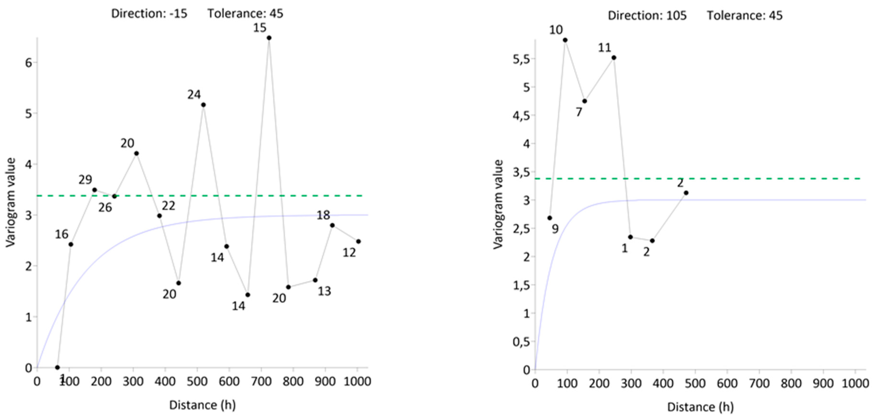
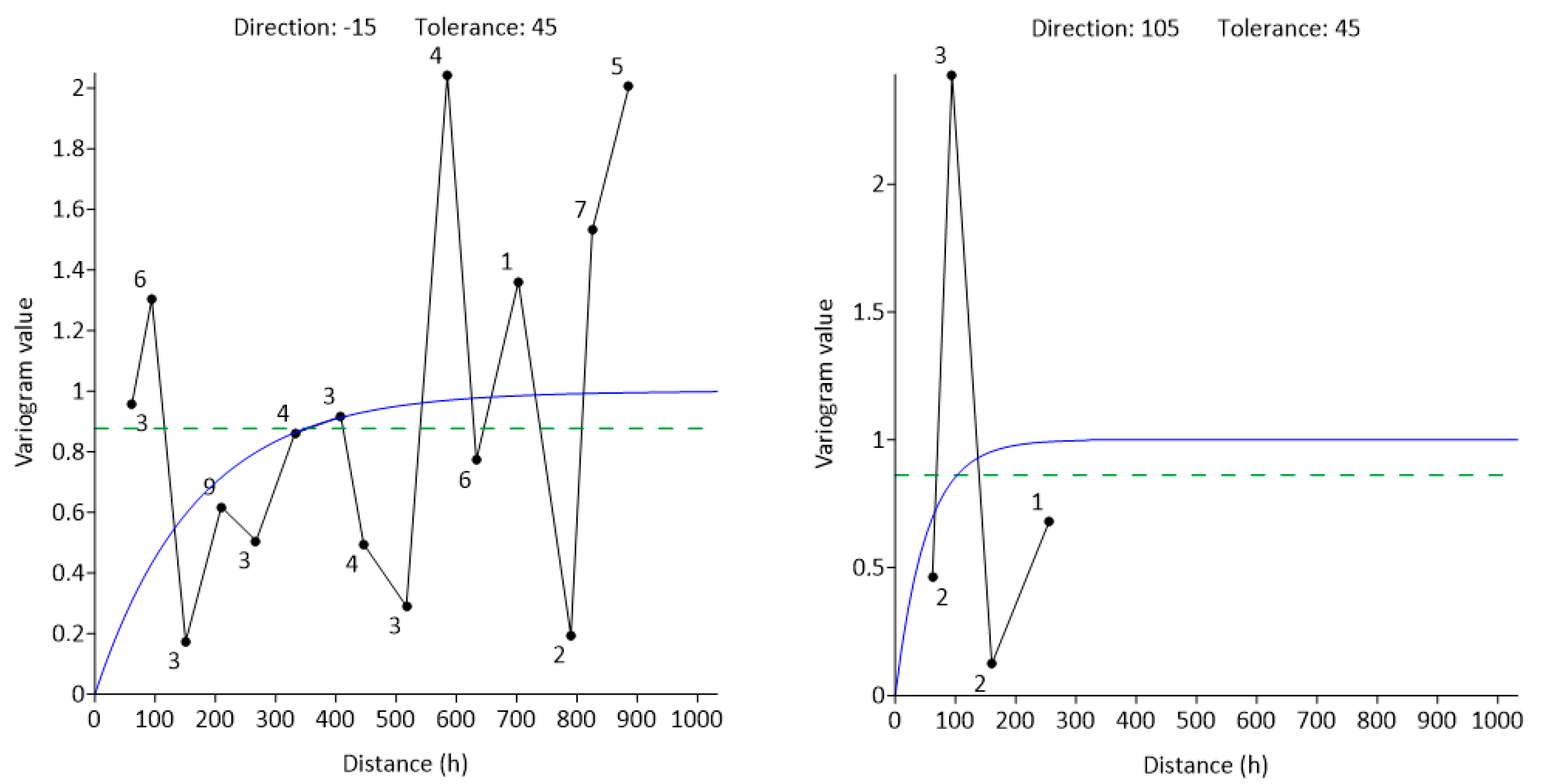
3.3. Kriging
- 2y(h)—variogram value
- n—number of data pairs at distance “h”
- z(xi)—value at location “xi”
- z(xi + h)—value at location distant for “h” from location “xi”
3.4. Inverse Distance Weighting
- ziu—estimated value
- di—distance to the “i-th” location
- zi—known value at the “i-th” location
- p—power exponent for distance
4. Results
5. Conclusions
Author Contributions
Funding
Acknowledgments
Conflicts of Interest
References
- Kerner, F.v. Geologische Spezijalkarte Der Oester. Ung. Mon., Zone 31, Kol XV, Blatt Sinj Und Spalato, 1:75,000—k.k. Geologische Reichsanstalt, 1914, Wien. Available online: https://www.hgi-cgs.hr/arhivske-karte-austrougarske (accessed on 22 March 2022).
- Kerner, F.v. Die Geologischen Verhältnisse Der Poljen von Blaca Und Konjsko Bei Spalato; Separatdruck; Geologisch-Paläontologisches Anstalt der Universität Basel: Basel, Switzerland, 1902. [Google Scholar]
- Kerner, F.v. Gliederung der Spalatiner Flyschformation, Verh. geol. R. A., 1903, Wien. Available online: https://www.zobodat.at/pdf/VerhGeolBundesanstalt_1903_0085-0087.pdf (accessed on 30 March 2022).
- Kerner, F.v. Zur geologie von Spalato (Entgegung an prof Carlo de Stefani und A. Martelli). Verh. geol. R. A., 1905, 16, Wien. Available online: https://www.zobodat.at/pdf/VerhGeolBundesanstalt_1905_0127-0165.pdf (accessed on 30 March 2022).
- Schubert, R. Geologische Fuhrer Durch Damatien, Sammlung geol. Fiihrer, 1909, 14, Berlin. Available online: https://opac.geologie.ac.at/ais312/dokumente/VH1909_234_A.pdf (accessed on 30 March 2022).
- Schubert, R. Geologija Dalmacije; Matica Dalmatinska: Zadar, Croatia, 1909. [Google Scholar]
- Marinčić, S. Paleogene breccias of the wider Mosor area. Geološki Vjesn. 1970, 23, 113–119. (In Croatian) [Google Scholar]
- Lukšić, B. Research for the Cement Industry in the Wider Area of Split—Quarry “Partizan”; 232, Zagreb; Fund p. while. Cemex Croatia d.d.: Kaštel Sućurac, Crotia, 1976. (In Croatian) [Google Scholar]
- Marinčić, S.; Korolija, B.; Mamužić, P.; Magaš, N.; Majcen, Ž.; Brkić, M.; Benček, Đ. Interpreter of the Basic Geological Map M 1: 100,000 for Omiš, K 33-22; Map: Beograd, Sebia, 1977. (In Croatian) [Google Scholar]
- Marinčić, S. Eocene flysch of the Adriatic belt. Geol. Vjesn. 1981, 34, 27–38. (In Croatian) [Google Scholar]
- Marjanac, T. Sedimentation of Kerner’s “middle flysch zone” (Paleogene, Split area). Geol. Vjesn. 1987, 40, 177–194. (In Croatian) [Google Scholar]
- Marjanac, T. Reflected sediment gravity flows and their deposits in flysch of Middle Dalmatia, Yugoslavia. Sedimentology 1990, 37, 921–929. [Google Scholar] [CrossRef]
- Tomašić, I. Limitation of contours of mineral raw materials in the deposit space with regard to quality. Rud.-Geol.-Naft. Zb. 1990, 2, 177–181, (In Croatian with English Abstract). [Google Scholar]
- Matijaca, M.; Vujec, S. Statistical interpretation of raw materials for the cement industry in Split. Rud.-Geol.-Naft. Zb. 1990, 2, 75–81, (In Croatian with English Abstract). [Google Scholar]
- Marjanac, T. Deposition of Megabeds (Megaturbidites) and Sea-Level Change in a Proximal Part of Eocene-Miocene Flysch of Central Dalmatia (Croatia). Geol. Boulder 1996, 24, 543–546. [Google Scholar] [CrossRef]
- Miščević, P.; Roje-Bonacci, T. Weathering process in eocene flysch in region of Split (Croatia). Rud.-Geol.-Naft. Zb. 2001, 13, 47–55. [Google Scholar]
- Pollak, D.; Buljan, R.; Toševski, A. Engineering-Geological and Geotechnical Properties of Flysch Formations in Kaštela Region. Građevinar 2010, 62, 8. [Google Scholar]
- Žižić, D.; Bartulović, H. Dietzsch cement kilns and their significance for the industrial architecture of Dalmatia. Prost. Znan. Časopis Arhit. Urban. 2015, 23, 42–55. (In Croatian) [Google Scholar]
- Parlov, J.; Hrženjak, P.; Bralić, N.; Terzić, J. Comparison of the Hydraulic Conductivities Calculated from Pumping Tests and Discontinuities in the Middle Eocene Flysch Basin, Exploitation Field Sv. Juraj-Sv. Kajo, Croatia. In Proceedings of the 42nd IAH Congress, Rome, Italy, 13–18 September 2015. [Google Scholar]
- Pencinger, V.; Ožanić, M.; Crnogaj, S.; Dedić, Ž.; Jurić, A. Study on the Reserves of Mineral Raw Materials for the Production of Cement in the Exploitation Field “St. Juraj—Sv. Kajo ”-Restoration; Croatian Geological Survey: Zagreb, Croatia, 2009. (In Croatian) [Google Scholar]
- Kruk, B.; Dedić, Ž. Study on the Reserves of Mineral Raw Materials for the Production of Cement in the Exploitation Field “St. Juraj—Sv. Kajo ”-Restoration; Croatian Geological Survey: Zagreb, Croatia, 2013. (In Croatian) [Google Scholar]
- Duda, W.H. Cement-Data-Book: International Process Engineering in the Cement Industry; Bauverlag: Gütersloh, Germany, 1985. [Google Scholar]
- Nornadiah, M.R.; Yap, B.W. Power comparisons of Shapiro-Wilk, Kolmogorov-Smirnov, Lilliefors and Anderson-Darling tests. J. Stat. Modeling Anal. 2011, 2, 21–33. [Google Scholar]
- Yazici, B.; Yolacan, S. A comparison of various tests of normality. J. Stat. Comput. Simul. 2007, 77, 175–183. [Google Scholar] [CrossRef]
- Malvić, T.; Medunić, G. Statistics in Geology. In Textbooks of the University of Zagreb; Faculty of Mining, Geology and Petroleum Engineering and Faculty of Science, University of Zagreb: Zagreb, Croatia, 2015; 88p. [Google Scholar]
- Kolmogorov-Smirnov Test Calculator: Normality Calculator, Q-Q Plot. Available online: https://www.statskingdom.com/kolmogorov-smirnov-test-calculator.html (accessed on 24 March 2022).
- Shapiro-Wilk Test Calculator: Normality Calculator, Q-Q Plot. Available online: https://www.statskingdom.com/shapiro-wilk-test-calculator.html (accessed on 24 March 2022).
- Dimitrova, D.S.; Kaishev, V.K.; Tan, S. Computing the Kolmogorov-Smirnov Distribution When the Underlying CDF Is Purely Discrete, Mixed, or Continuous. J. Stat. Softw. 2020, 95, 1–42. [Google Scholar] [CrossRef]
- Šapina, M.; Vekić, M. New lithostratigraphic units of the Croatian coast and their provisions in the “R” programming language. Rud.-Geol.-Naft. Zb. 2015, 30, 13–24, (In Croatian with English Abstract). [Google Scholar] [CrossRef] [Green Version]
- Shapiro, S.S.; Wilk, M.B. An analysis of variance test for normality (complete samples). Biometrika 1965, 52, 591–611. [Google Scholar] [CrossRef]
- Malvić, T.; Cvetković, M.; Balić, D. Geomathematic Dictionary; Croatian Geological Society: Zagreb, Croatia, 2008; 74p. (In Croatian) [Google Scholar]
- Mesić Kiš, I. Comparison of ordinary and universal kriging interpolation techniques on a depth variable (a case of linear spatial trend), case study of the Šandrovac field. Rud.-Geol.-Naft. Zb. 2016, 31, 2. [Google Scholar] [CrossRef]
- Malvić, T. Application of Statistics in the Analysis of Geological Data. In Textbooks of the University of Zagreb; INA-Oil Industry d.d.: Zagreb, Croatia, 2008; 103p. [Google Scholar]
- Malvić, T.; Ivšinović, J.; Velić, J.; Sremac, J.; Barudžija, U. Application of the Modified Shepard’s Method (MSM): A Case Study with the Interpolation of Neogene Reservoir Variables in Northern Croatia. Stats 2020, 3, 68–83. [Google Scholar] [CrossRef] [Green Version]
- Malvić, T.; Ivšinović, J.; Velić, J.; Rajić, R. Interpolation of Small Datasets in the Sandstone Hydrocarbon Reservoirs, Case Study of the Sava Depression, Croatia. Geoscience 2019, 9, 201. [Google Scholar] [CrossRef] [Green Version]


| Layer | Lithological Unit | Top layer (m) | Botom Layer (m) | Layer Thickness (m) | Data Number (−) |
|---|---|---|---|---|---|
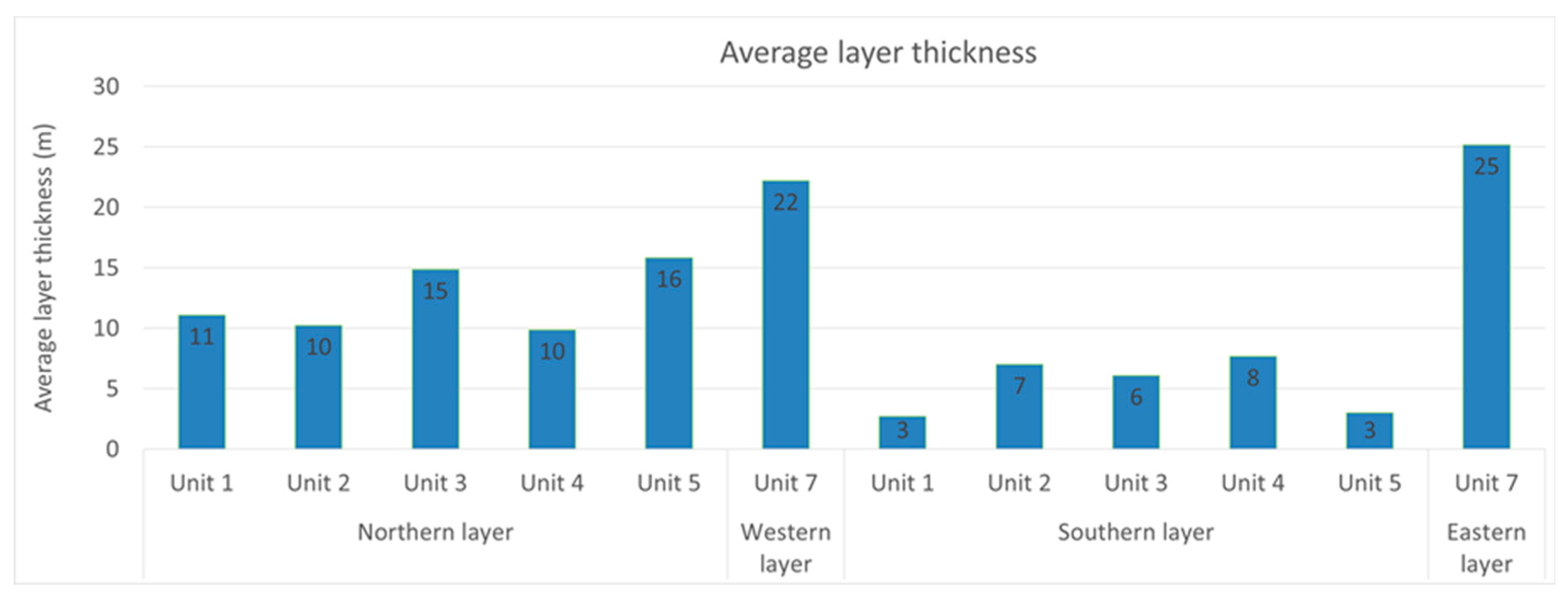
| North layer | Change between marl, sandstone with alternation of conglomerates | 159 | 148 | 11 | 36 |
| Clayey marl | 135 | 125 | 10 | 18 | |
| Marl | 130 | 115 | 15 | 26 | |
| Calcsiltite | 120 | 110 | 10 | 28 | |
| Calcarenite | 105 | 89 | 16 | 18 | |
| Western layer | Debrites | 102 | 78 | 22 | 7 |
| South layer | Change between marl, sandstone with alternations of conglomerates | 96 | 93 | 3 | 7 |
| Clayey marl | 101 | 94 | 7 | 27 | |
| Marl | 101 | 95 | 6 | 14 | |
| Calcsiltite | 105 | 97 | 8 | 24 | |
| Calcarenite | 103 | 100 | 3 | 4 | |
| Eastern layer | Debrites | 119 | 89 | 25 | 5 |
| Ʃ = 214 |
| Lithological Unit | Statistic | Mapping | ||||||
|---|---|---|---|---|---|---|---|---|
| CaO (%) | SiO2 (%) | LSF (−) | ||||||
| Data Number (n) | Normality Test | Test Outcome | Interpolation Method | Test Outcome | Interpolation Method | Test Outcome | Interpolation Method | |
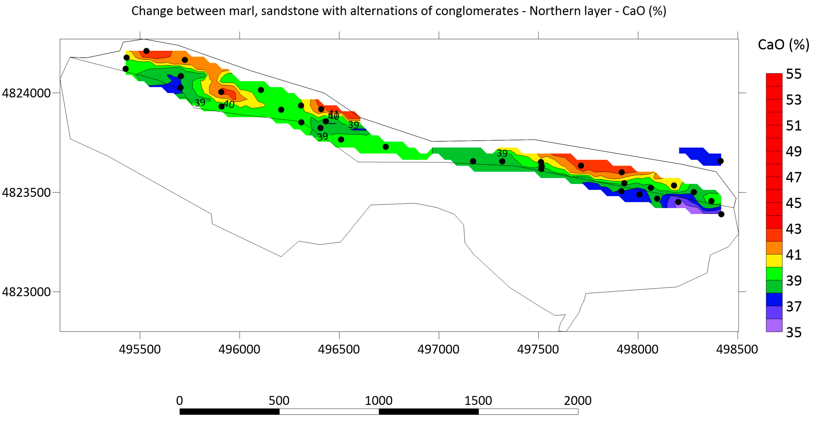
| Change between marl, sandstone with alternations of conglomerates—norther layer | 36 | SW | Pass | OK | Pass | OK | Pass | OK |
| Calcarenite—northern layer | 18 | KS | Pass | OK | Pass | OK | Pass | OK |
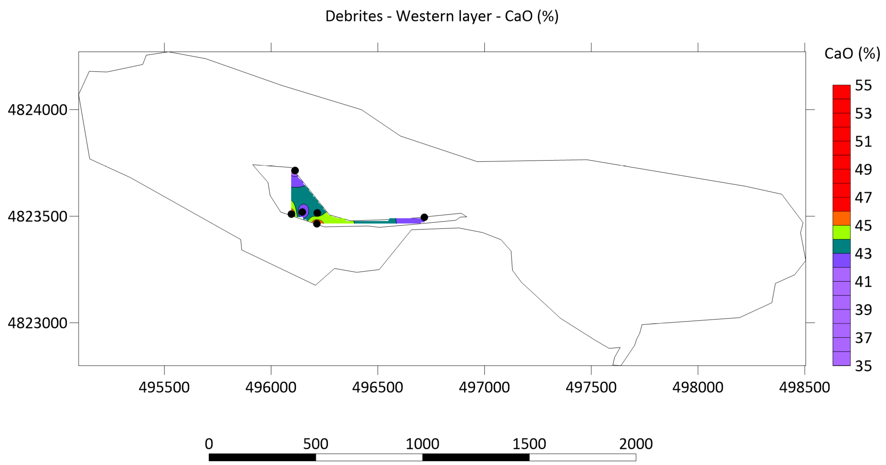
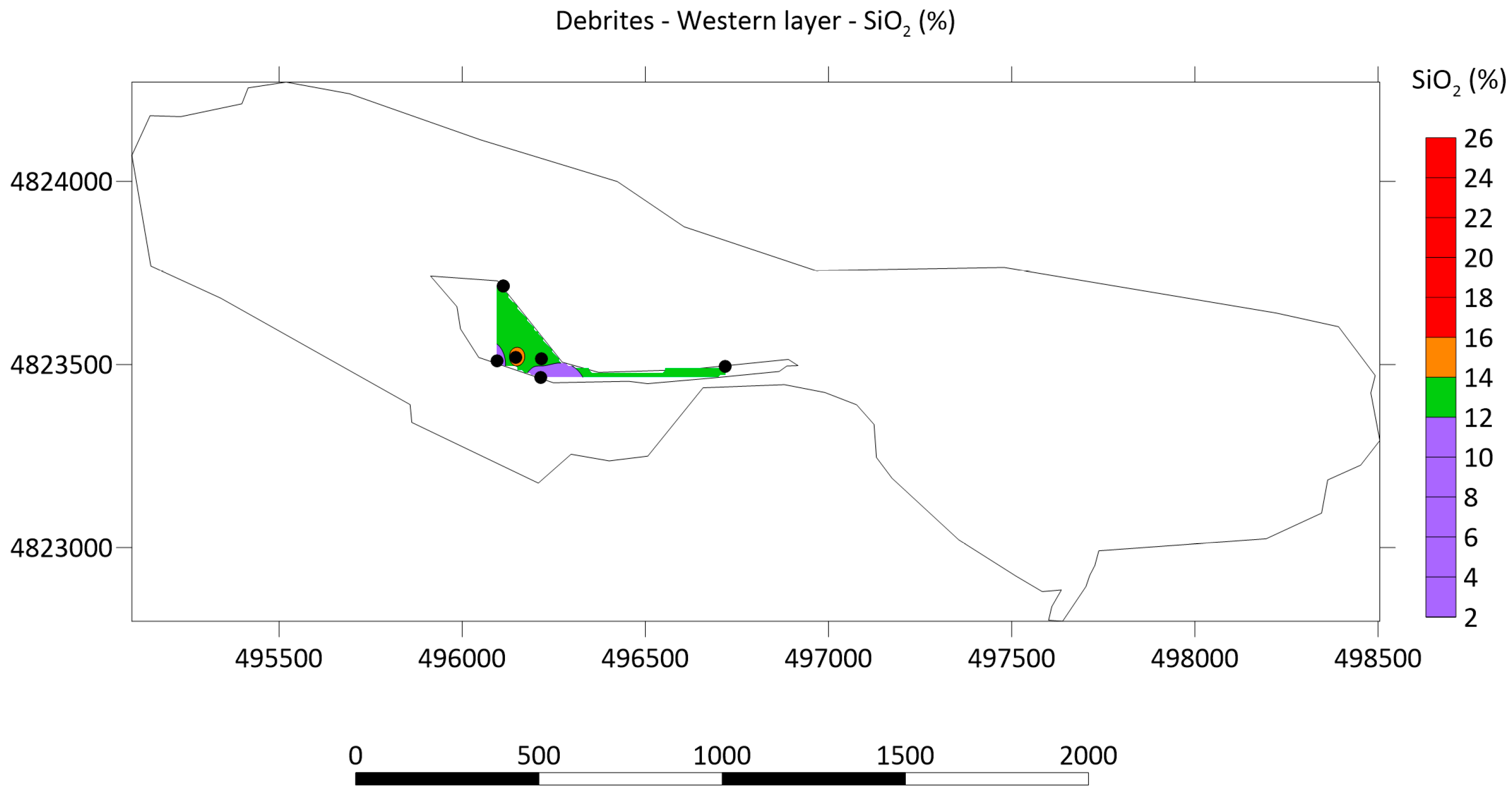
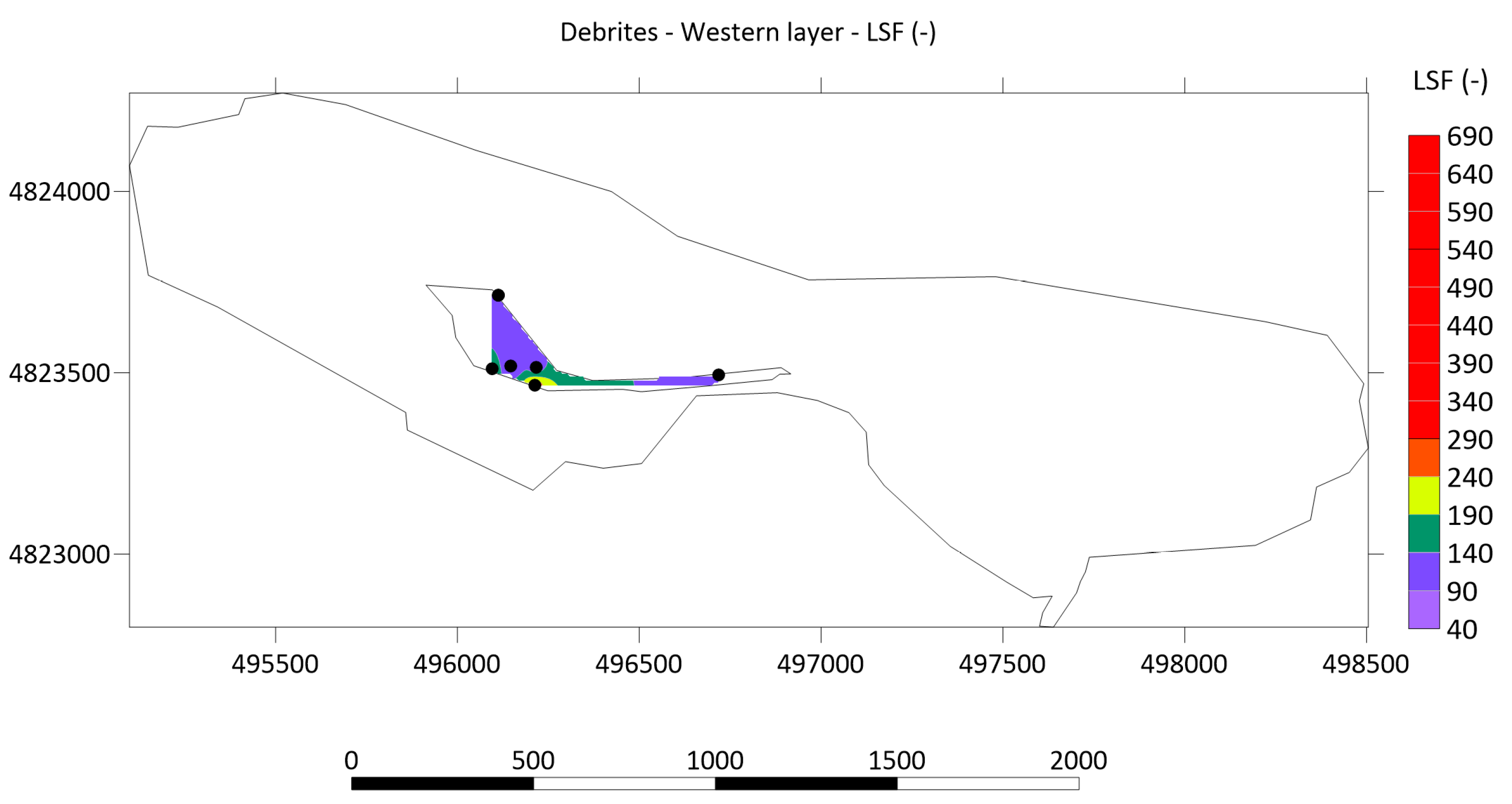
| Debrites—western layer | 7 | KS | Pass | IDW | Pass | IDW | Fail | IDW |
| Lithological Units | Chemical Characteristics | Cement Modules | Pass Rate | |||||||||||
|---|---|---|---|---|---|---|---|---|---|---|---|---|---|---|
| SiO2 | Al2O3 | Fe2O3 | CaO | MgO | SO3 | Na2O | K2O | CaCO3 | LSF | SM | AM | |||
| Change between marl, sandstone with alternations of conglomerates—northern layer | SW test | + | + | + | + | + | − | + | − | + | + | − | − | 67% |
| n = 36; α = 0.05 | ||||||||||||||
| p | 0.2848 | 0.3077 | 0.0827 | 0.1800 | 0.0577 | 0.0436 | 0.0776 | 0.0180 | 0.1803 | 0.1783 | 0.0000 | 0.0007 | ||
| Change between marl, sandstone with alternations of conglomerates—southern layer | KS test | + | + | + | − | − | + | + | + | − | − | − | + | 58% |
| n = 8; α = 0.05 | ||||||||||||||
| p | 0.0652 | 0.0784 | 0.0963 | 0.0194 | 0.0183 | 0.3973 | 0.3802 | 0.0791 | 0.0198 | 0.0257 | 0.0162 | 0.7911 | ||
| Clayey marl—northern layer | KS test | + | + | + | + | + | + | + | − | + | + | − | + | 83% |
| n = 18; α = 0.05 | ||||||||||||||
| p | 0.4312 | 0.6364 | 0.8022 | 0.8059 | 0.0849 | 0.1441 | 0.8625 | 0.0000 | 0.8008 | 0.5899 | 0.0321 | 0.1137 | ||
| Clayey marl—southern layer | KS test | + | + | + | + | + | + | + | − | + | + | − | − | 75% |
| n = 27; α = 0.05 | ||||||||||||||
| p | 0.0881 | 0.0723 | 0.2051 | 0.4998 | 0.2029 | 0.2989 | 0.1453 | 0.0001 | 0.4935 | 0.4322 | 0.0000 | 0.0002 | ||
| Marl—northern layer | KS test | − | + | − | − | + | − | + | − | − | − | − | − | 25% |
| n = 26; α = 0.05 | ||||||||||||||
| p | 0.0004 | 0.0632 | 0.0354 | 0.0022 | 0.1178 | 0.0002 | 0.3153 | 0.0000 | 0.0021 | 0.0060 | 0.0276 | 0.0000 | ||
| Marl—southern layer | KS test | + | + | + | + | + | + | − | − | + | + | + | + | 83% |
| n = 14; α = 0.05 | ||||||||||||||
| p | 0.2608 | 0.1904 | 0.0677 | 0.3273 | 0.1078 | 0.5297 | 0.0491 | 0.0000 | 0.3299 | 0.5425 | 0.1851 | 0.1065 | ||
| Calcsiltite—northern layer | KS test | + | + | + | + | + | − | − | − | + | + | + | − | 67% |
| n = 28; α = 0.05 | ||||||||||||||
| p | 0.7297 | 0.6069 | 0.4000 | 0.7610 | 0.4963 | 0.0000 | 0.0015 | 0.0002 | 0.7595 | 0.7079 | 0.1044 | 0.0003 | ||
| Calcsiltite—southern layer | KS test | − | − | + | + | + | − | + | − | + | − | − | − | 42% |
| n = 24; α = 0.05 | ||||||||||||||
| p | 0.0170 | 0.0021 | 0.7666 | 0.1105 | 0.2280 | 0.0105 | 0.6101 | 0.0029 | 0.1128 | 0.0044 | 0.0000 | 0.0343 | ||
| Calcarenite—northern layer | KS test | + | + | + | + | + | + | − | + | + | + | − | − | 75% |
| n = 18; α = 0.05 | ||||||||||||||
| p | 0.1573 | 0.8429 | 0.2380 | 0.8252 | 0.3341 | 0.0550 | 0.0192 | 0.0736 | 0.8188 | 0.4630 | 0.0243 | 0.0002 | ||
| Calcarenite—southern layer | KS test | + | + | + | + | + | − | + | + | + | + | + | + | 92% |
| n = 4; α = 0.05 | ||||||||||||||
| p | 0.2607 | 0.7948 | 0.2787 | 0.2413 | 0.1976 | 0.0107 | 0.6603 | 0.9273 | 0.2400 | 0.2216 | 0.3421 | 0.3788 | ||
| Debrites—western layer | KS test | + | + | + | + | + | + | + | + | + | − | + | + | 92% |
| n = 7; α = 0.05 | ||||||||||||||
| p | 0.6479 | 0.1508 | 0.2862 | 0.5895 | 0.1094 | 0.6915 | 0.3960 | 0.2639 | 0.6201 | 0.0280 | 0.2487 | 0.2891 | ||
| Debrites—eastern layer | KS test | + | + | + | + | + | + | + | − | + | + | + | + | 92% |
| n = 5; α = 0.05 | ||||||||||||||
| p | 0.6430 | 0.7450 | 0.3448 | 0.0871 | 0.8986 | 0.3906 | 0.5844 | 0.0494 | 0.0879 | 0.7707 | 0.6347 | 0.3404 | ||
| Passrate | 83% | 92% | 92% | 83% | 92% | 58% | 75% | 33% | 83% | 67% | 42% | 50% | 71% | |
Publisher’s Note: MDPI stays neutral with regard to jurisdictional claims in published maps and institutional affiliations. |
© 2022 by the authors. Licensee MDPI, Basel, Switzerland. This article is an open access article distributed under the terms and conditions of the Creative Commons Attribution (CC BY) license (https://creativecommons.org/licenses/by/4.0/).
Share and Cite
Bralić, N.; Malvić, T. Interpretation of Chemical Analyses and Cement Modules in Flysch by (Geo)Statistical Methods, Example from the Southern Croatia. Processes 2022, 10, 813. https://doi.org/10.3390/pr10050813
Bralić N, Malvić T. Interpretation of Chemical Analyses and Cement Modules in Flysch by (Geo)Statistical Methods, Example from the Southern Croatia. Processes. 2022; 10(5):813. https://doi.org/10.3390/pr10050813
Chicago/Turabian StyleBralić, Nikolina, and Tomislav Malvić. 2022. "Interpretation of Chemical Analyses and Cement Modules in Flysch by (Geo)Statistical Methods, Example from the Southern Croatia" Processes 10, no. 5: 813. https://doi.org/10.3390/pr10050813