A Novel Graphical Targeting Technique for Optimal Allocation of Biomass Resources

Abstract

Biomass has gained global attention as one of the most important renewable energy resources that reduces greenhouse gas emissions. Various research works have been dedicated to biomass supply chain in the past decade as to continuously support the deployment of biomass resources for regional applications. In this work, a novel graphical method based on process integration is proposed for targeting the amount of biomass resources needed for a power generation problem. Apart from having a good visualized interface, the graphical method provides good insights to stakeholders on the macro-level planning of biomass allocation. Two examples are solved to demonstrate the newly proposed methods.

1. Introduction

The Global Energy Review 2021 [1] projected that the global energy demand was expected to increase by 4.6% in year 2021. This rise in global energy demand is primarily fuelled by fossil-based sources. Nevertheless, the global awareness of reducing greenhouse gas emissions (particularly CO₂) has encouraged the development of low-CO₂ renewable energy resources. In year 2020, the renewable energy sector reported a contribution of 29% to the global electricity generation, i.e., a growth of 3% despite the global lock down due to the COVID-19 pandemic [1]. Along with solar and hydropower, biomass is among the most important renewable energy sources for sustainable electricity generation.

Biomass supply chain consists of various activities involving the supply of biomass, their transportation, storage, conversion, and delivery of their value-added products [2]. One of the most important value-added biomass products is arguably biofuel/bioenergy. As reported by Lim et al. [3], various challenges are accounted for in the biomass supply chain for biofuel production; these include the variation in biomass availability, distinct characteristics of each biomass species, uncertain technology performance, logistics and transportation issues. Hence, various process system engineering tools were developed in the past two decades to address the various challenges encountered in biofuel and biomass supply chain. For instance, some earlier works which are based on mathematical programming models were proposed to synthesise regional bioenergy supply chain [4,5]. In the work by Ling et al. [6], centralized and decentralized technologies were considered for bioelectricity supply chain. In a more recent work, a stochastic model was proposed for co-firing biomass supply chain networks [7]. In some recent works, optimization models were developed with the objective to reduce CO₂ footprint [8,9].

Apart from the above-mentioned techniques, a widely accepted group of systematic tools for optimum planning of resources is arguably process integration. The latter consists of some useful graphical techniques that were commonly utilised for the conservation of materials [10,11] and energy resources [12,13] in the chemical processing industries. In recent years, these graphical tools have also been extended for optimal synthesis of biomass supply chain. In the seminal work of Lam et al. [14], the Regional Energy Surplus–Deficit Curves were proposed to synthesise a biomass supply chain with the aim to minimise its carbon footprint. In another later work by Tan et al. [15], a graphical pinch diagram was extended for the optimal planning of a biochar network. Graphical approaches are always regarded as handy tools welcomed by industrial sectors, as they provide good insights to the problem due to its intuitive nature. Furthermore they are often used to facilitate discussion among team members. To date, however, no graphical approach has been reported for the allocation of biomass resources for power generation. Note that the earlier developed graphical techniques (e.g., [14,15]) cannot be used directly for biomass allocation, as they do not consider the unique characteristics of biomass that are important for power generation, e.g., moisture content, calorific values, etc. Hence, a new graphical technique that incorporates biomass characteristics is to be developed. This is the main subject of this work.

In this work, a novel graphical pinch diagram is presented to identify the optimal allocation of biomass resources for power generation. In particular, the novel graphical tool helps to identify the exact amount of biomass resources needed to fulfil the targeted power output of some power plants. The paper is structured as follows. In the next section, a formal problem statement is given. This is then followed by the power generation model, and the procedure for plotting the graphical pinch diagram. Two examples on bioenergy generation are used for demonstrating the novel graphical diagram.

2. Problem Statement

The problem to be addressed is formally stated as follows:

▪

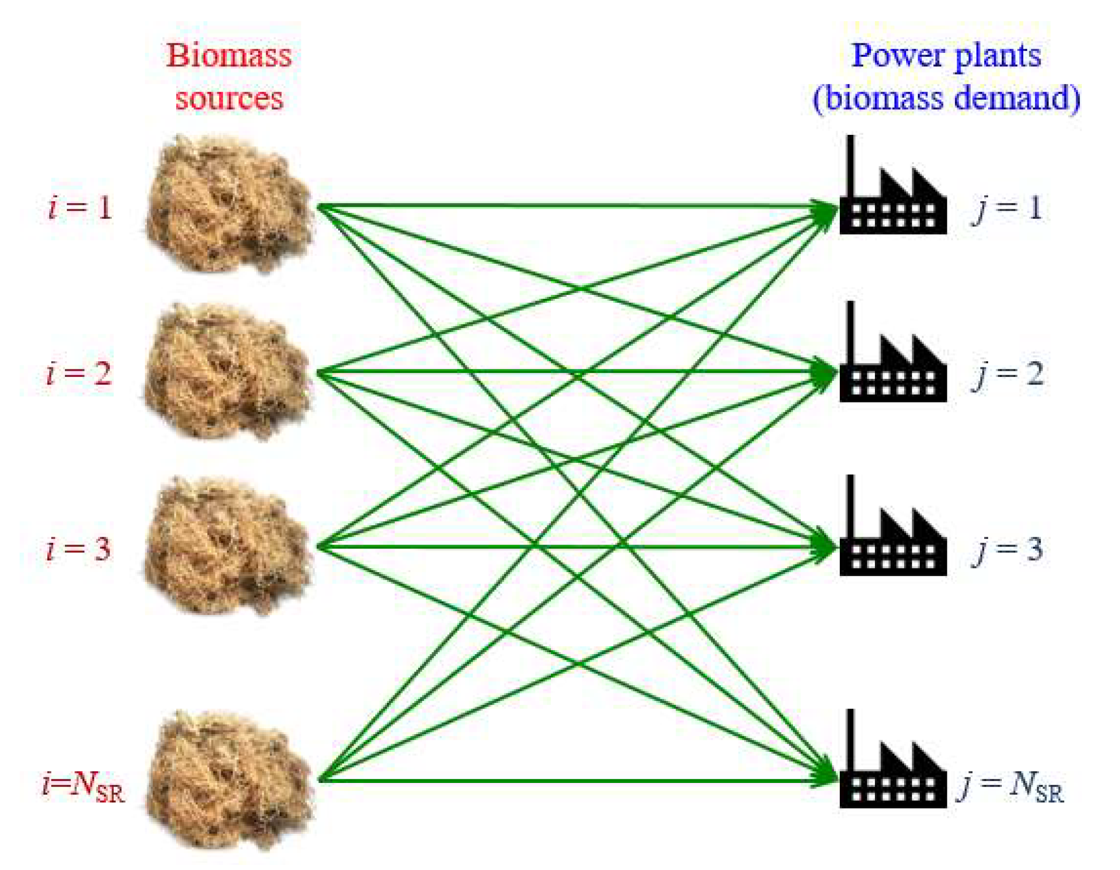
Given a set of biomass sources i ∈ I. Each biomass type has its specific calorific value CV_i, moisture content MC_i and maximum availability S_i.

▪

The biomass sources are to be allocated to a set of biomass demands j ∈ J, which are power plants that require biomass for power generation. Each plant has its power output P_j that has to be fulfilled and can only handle a maximum capacity D_j of biomass.

The biomass allocation problem can be described by a superstructure diagram in Figure 1. The objective of this work is to determine the optimum allocation of biomass source i to power plant j.

3. Power Generation Model

To determine the biomass requirement for power generation, the model in Foo et al. [5] is adopted. For power plant j with output $P_j$, its steam requirement for the turbine ($ST{M}_j$) may be calculated using Equation (1).

$$ST{M}_j=\frac{P_j}{{\eta }_{Turb}{\hat{H}}_{Turb}}$$

(1)

where ${\eta }_{Turb}$ and ${\hat{H}}_{Turb}$ are efficiency (%) and enthalpy (kJ/kg) for turbine calculation.

To generate the required amount of steam for the turbine, a boiler is to be used. The biomass requirement for power plant j ($D_j$) is hence calculated using Equation (2).

$$D_j=\frac{ST{M}_j{\hat{H}}_{\mathrm{Boil}}}{C{V}_{\mathrm{Biom}}S{C}_{\mathrm{Biom}}{\eta }_{\mathrm{Boil}}}$$

(2)

where ${\eta }_{\mathrm{Boil}}$ and ${\hat{H}}_{\mathrm{Boil}}$ are efficiency (%) and enthalpy (kJ/kg) for boiler calculation, while $C{V}_{\mathrm{Biom}}$ and $S{C}_{\mathrm{Biom}}$ are average calorific value (kJ/kg) and solid content (wt%) of biomass, calculated based on average value of the various biomass types that are fed to the power plant. Note also that solid content can be calculated from moisture content (MC_Biom, wt%) that is more commonly used in the biomass industry.

Equations (1) and (2) may be combined and rearranged to the form in Equation (3).

$$P_j=C_j{D}_j$$

(3)

In Equation (3), $C_j$ is characterised as the power generation factor for power plant j, given as in Equation (4).

$$C_j=\frac{{\eta }_{\mathrm{Turb}}{\hat{H}}_{\mathrm{Turb}}C{V}_{\mathrm{Biom}}S{C}_{\mathrm{Biom}}{\eta }_{\mathrm{Boil}}}{{\hat{H}}_{\mathrm{Boil}}}$$

(4)

Similar correlations may be expressed for power output (P_i, Equation (5)) and the generation factor (C_i, Equation (6)) for biomass i:

$$P_i=C_i{S}_i$$

(5)

$$C_i=\frac{{\eta }_{Turb}{\hat{H}}_{Turb}C{V}_{i}S{C}_i{\eta }_{Boil}}{{\hat{H}}_{Boil}}$$

(6)

where $C{V}_i$ and $S{C}_i$ are calorific value (kJ/kg) and solid content (wt%) of biomass i. Note also that solid content of biomass can be calculated from its moisture content (MC_i, wt%) easily.

Graphical Targeting Method

A novel graphical tool is presented here, known as the bioenergy pinch diagram (BEPD). Steps for plotting the BEPD are given as follows.

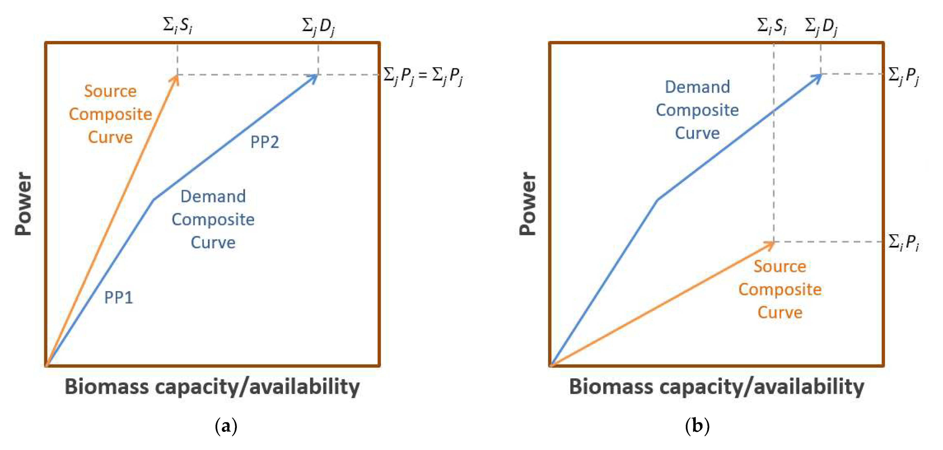
• A demand composite curve is first plotted on a power versus biomass capacity diagram (Figure 2a). The demand composite curve consists of the individual power plants that require biomass feed. Its horizontal distance represents the maximum total capacity of biomass that can be handled by these plants (Σ_jD_j), while its vertical distance represents their total power output (Σ_jP_j). Note that the individual segments in the demand composite curve correspond to power plant j (PP1 and PP2 in Figure 2a) which have been arranged according to the descending order of their power generation factor C_j (slope of the segment), the latter may be calculated using Equation (4).
• A source composite curve is next plotted on the same diagram as the demand composite curve, but is interpreted as power versus biomass handling capacity. The source composite curve may consist of one or more biomass sources, plotted according to the descending order of their power generation factor C_i (determined using Equation (6)). The BEPD is considered feasible when the source composite curve is located to the left of the demand composite curve and has, at least, the same vertical distance as the latter, such as that shown in Figure 2a. For this case, the source composite curve will generate a total power of Σ_iP_i, which matches the total output of the power plants (Σ_jP_j), and yet is lower than their maximum total handling capacity (i.e., Σ_iS_i ≤ Σ_jD_j).
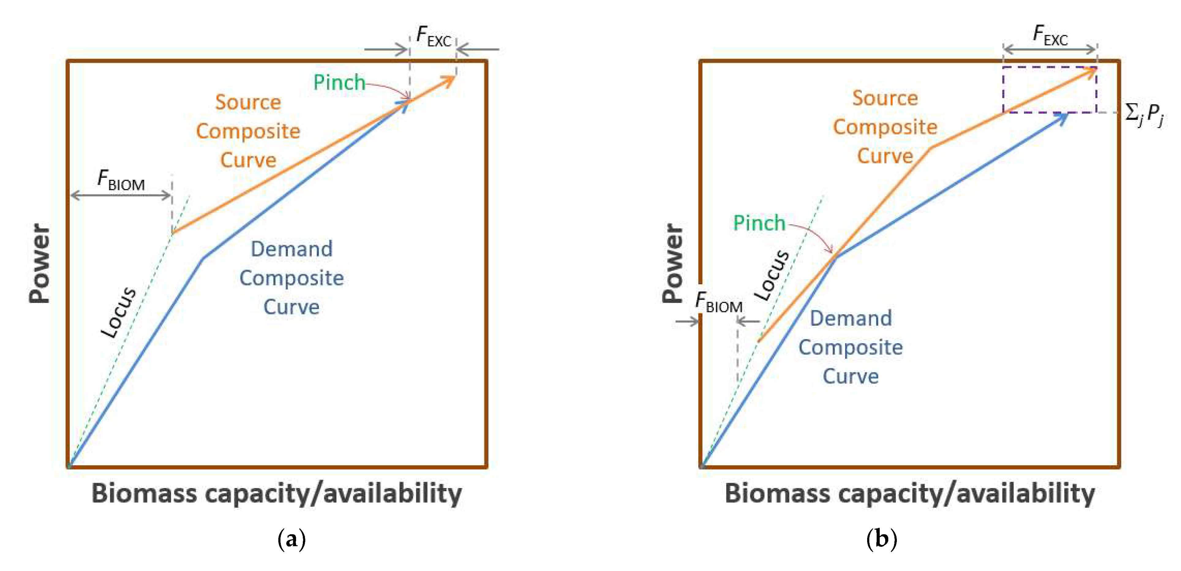
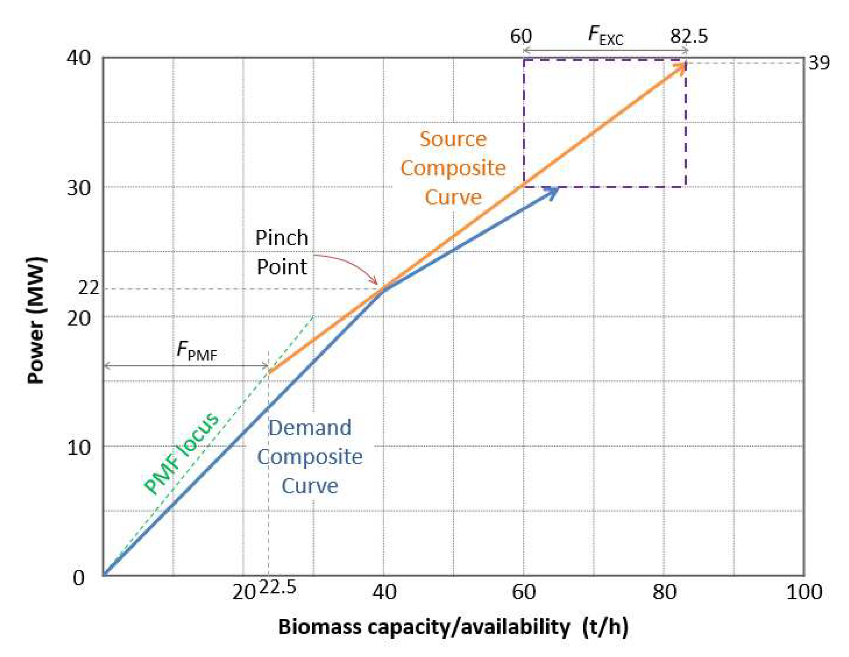
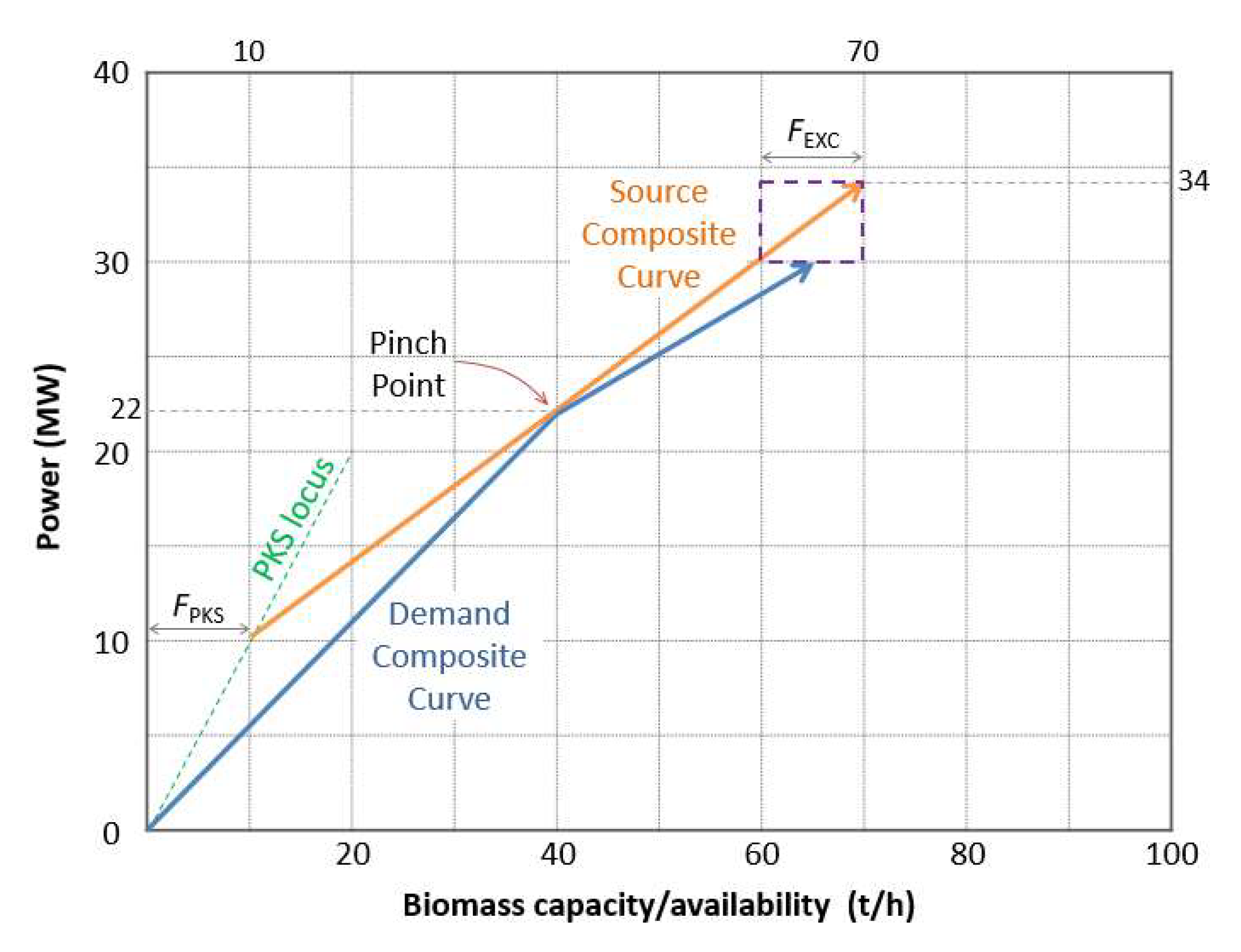
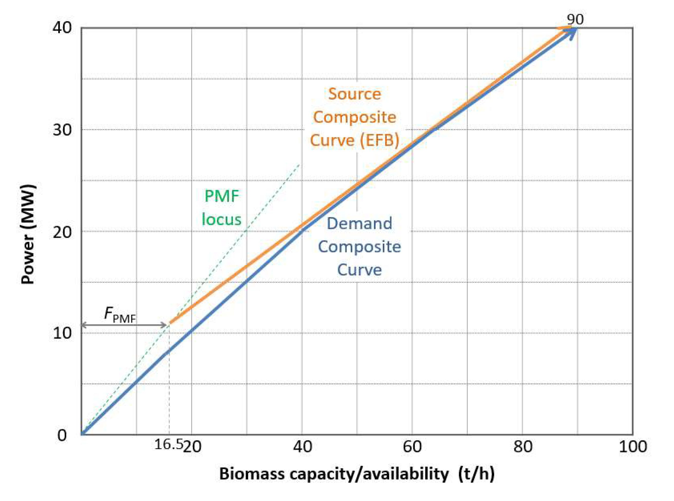
• In cases where the source composite curve is found on the right and/or below the demand composite curve (such as that in Figure 2b), the BEPD is considered infeasible. Additional biomass with a higher power generation factor is to be supplied in order to restore its feasibility. As shown in Figure 3a, additional biomass with higher power generation factor is added; the latter is characterised by its locus of steeper slope. The source composite curve is then slid along this locus until it stays completely above and to the left of the demand composite curve and touches the former at the pinch. The opening on the left of the BEPD represents the minimum amount of additional biomass to be added (F_BIOM). Its amount is to be minimised, as it is usually more expensive due to its higher power generation factor. Conversely, the opening on the right of the BEPD represents excess biomass (F_EXC) that is beyond the handling capacity of the power plant. This excess biomass can be utilised for other commercial purposes. Note that there are cases where the source composite curve is comprised of several source segments. Besides, there are also cases where the pinch occurs in the middle section of the composite curves. Both of these cases are shown in Figure 3b. The same principles are applied here. The source composite curve is slid along the locus of biomass with higher power generation factor, until it stays completely above and to the left of the demand composite curve. The composite curves touch each other at the pinch. For this case, excess biomass (F_EXC) is determined from the horizontal distance of the segment extended beyond the demand composite curve (represented by the rectangular box in Figure 3b).

The BEPD is next demonstrated with two examples on biomass allocation planning.

4. Illustrative Examples

Two examples are used here to elucidate the newly proposed graphical method. For both examples, the important parameters for power generation are given in

Table 1. Important parameters for power generation.

Parameters	Values
Turbine
$\mathrm{Turbine} \mathrm{efficiency}, {\eta }_{\mathrm{Turb}}$	19.8%
$\mathrm{Enthalpy} \mathrm{of} \mathrm{steam}, {\hat{H}}_{\mathrm{Turb}}$	3140 kg/kg steam
Boiler
$\mathrm{Boiler} \mathrm{efficiency}, {\eta }_{\mathrm{Boil}}$	85%
$\mathrm{Enthalpy} \mathrm{of} \mathrm{steam}, {\hat{H}}_{\mathrm{Boil}}$	2669 kJ/kg steam
$\mathrm{Average} \mathrm{calorific} \mathrm{value} \mathrm{of} \mathrm{biomass}, C{V}_{\mathrm{Biom}}$	19,000 kJ/kg biomass

, while the moisture content tolerated by the power plants is given in the respective examples.

4.1. Example 1—Single Biomass Source

In Example 1, two biomass power plants (PP1 and PP2) are analysed, with their data given in

Table 2. Data for power plants in Example 1.

Power Plants	Pj (MW)	MCBiom (%)	Dj (t/h)	Cj (MWh/t)
PP1	22	47.4	40	0.55
PP2	8	69.4	25	0.32
Total	30		65

. As shown, the individual plants were designed based on their respective average moisture content (MC_Biom), which may be converted as solid content (SC_Bio = 100% − MC_Bio) to be used in Equation (2). Their demand of biomass (D_j) can be calculated using Equation (1), while their power generation factors are calculated using Equation (4), listed in the last two columns of Table 2.

Three types of biomass are available for use, i.e., palm kernel shell (PKS), empty fruit bunch (EBB) and palm mesocarp fibre (PMF), with their data shown in

Table 3. Data for biomass in Example 1.

Biomass Types	Si (t/h)	CVi (kJ/kg)	MCi (%)	Pi (MW)	Ci (MWh/t)
PKS	To be determined	19,700	23	To be determined	1
PMF		19,000	36		0.67
EFB	60	18,700	61	24	0.4

. As shown, each biomass type has its CV and MC values. With given flowrate, their power output and generation factors can be determined using Equation (6), as shown in the last two columns of Table 3. Note however for this case, only two biomass types should be considered due to logistic concern. Among them, the EFB with the lowest CV value (lowest cost) is prioritised. The task is to determine the minimum amount of biomass with higher power generation factor, i.e., PKS or PMF.

Next, the BEPD was plotted following steps 1 and 2 of the procedure, with only EFB being used to construct the source composite curve. Figure 4 shows that the resulting BEPD is infeasible, as the source composite curve stays at the right of the demand composite curve. As shown, the EFB can only generate a power output of 24 MW (a total of 30 MW is required), but its supply is beyond the capacity limit of the power plant.

To restore the feasibility, the PMF is used. Its locus is first added to the BEPD, with a slope corresponding to its power generation factor (0.67 MW/t/h). Step 3 of the BEPD procedure is then followed. The source composite curve is slid along the locus until it stays entirely above and to the left of the demand composite curve, and touches the latter at the pinch. This results in a feasible BEPD (Figure 5), with minimum use of PMF (F_PMF), i.e., 22.5 t/h. The excess biomass (F_EXC), i.e., EFB, is determined from the horizontal distance of the rectangular box beyond the demand composite curve, i.e., 22.5 t/h (= 82.5 − 60 t/h); this excess biomass can be used for other commercial purposes. The overlapping region of the composite curves determines the amount of EFB to be utilised for power generation, i.e., 37.5 t/h (= 60 − 22.5 t/h).

One may also explore the use of PKS that has a higher CV value (and is more expensive). Replotting the BEPD by sliding the source composite curve on the steeper locus of PKS (due to its higher power generation factor of 1 MW/t/h), results in a feasible BEPD (Figure 6). As shown, both the minimum use of PKS (F_PKS) and excess EFB (F_EXC = 70 − 60 t/h) are determined as 10 t/h, which are both lower than the case in Figure 5. Furthermore, a higher amount of EFB (60 − 10 = 50 t/h) is utilised for power generation in this case. Detailed evaluation may be carried out to determine which allocation scheme is to be adopted based on their economic performance.

4.2. Example 2—Multiple Biomass Sources

In this example, four power plants are analysed, with their data shown in

Table 4. Data for power plants in Example 2.

Power Plants	Pj (MW)	MCj (%)	Dj (t/h)	Cj (MWh/t)
PP1	8	49.0	15	0.53
PP2	12	54.0	25	0.48
PP3	10	60.0	24	0.42
PP4	10	63.2	26	0.38
Total	40		90

. Three scenarios are analysed here, each with a different amount of palm biomass used, with data shown in

Table 5. Data for biomass in Example 2.

Scenario	Biomass Types	Si (t/h)	CVi (kJ/kg)	MCi (%)	Pi (MW)	Ci (MWh/t)
1	PKS	40	19,700	23	40	1
	EFB	100	18,700	61	40	0.4
2	PMF	To be determined	19,000	36	To be determined	0.67
	EFB	72.5	18,700	61	29	0.4
3	PKS	To be determined	19,700	23	To be determined	1
	PMF	18	19,000	36	12	0.67
	EFB	20	18,700	61	8	0.4

.

In Scenario 1, only single biomass is to be used for power generation. Figure 7 shows that the BEPD is infeasible, if EFB is used. Although sufficient EFB (100 t/h) can be used to generate the required power of 40 MW, the amount of biomass is beyond the handling capacity of the power plants (90 t/h). Conversely, if 40 t/h PKS is used, the BEPD shows that the power plants can fulfil the required power output of 40 MW, while the biomass supply rate (40 t/h) is lower than their handling capacity.

In Scenario 2, two types of biomass may be used, with EFB being prioritised. The BEPD in Figure 8 shows that 16.5 t/h of PMF is to be used, as the EFB alone is insufficient to cater the desired power output (40 MW) from the power plants. A similar situation also occurs in Scenario 3 where three biomass types are used. As shown in the BEPD in Figure 9, EFB and PMF are completely consumed, while 20 t/h of PKS is added to produce a total power output of 40 MW. For Scenario 3, no excess biomass sources are reported.

5. Practical Implications

The new graphical targeting technique in this work serves as a handy planning tool for biomass industrial practitioners in their day-to-day operation. Although both examples make use of palm biomass resources, other types of biomass resources (e.g., wood, rice rusk) may also be used, as long as their biomass characteristics (calorific value, moisture content, etc.) are given. Finally, note that the above problems may be solved using the superstructural model as presented in Appendix A.

6. Conclusions

A novel graphical targeting method is proposed in this work for the optimal allocation of biomass resources, based on process integration principles. Two examples based on palm biomass were used to elucidate the newly proposed method. In both examples, biomass with lower power generation factor were prioritised, while those of higher power generation factor were minimised. Although the examples are based on palm biomass, the same principles are applied to other types of biomass resources that may be used for power generation. Future works should look at other environmental aspects of biomass resources, such as water and land footprints.

References

- IEA. Global Energy Review 2021. Assessing the Effects of Economic Recoveries on Global Energy Demand and CO2 Emissions in 2021; IEA: Paris, France, 2021. [Google Scholar]
- Ng, W.P.Q.; How, B.S.; Lim, C.H.; Ngan, S.L.; Lam, H.L. Biomass supply chain synthesis and optimization. In Value-Chain of Biofuels; Yusup, S., Rashidi, N.A., Eds.; Elsevier: Amsterdam, The Netherlands, 2021; pp. 445–479. [Google Scholar] [CrossRef]
- Lim, C.H.; Ngan, S.L.; Ng, W.P.Q.; How, B.S.; Lam, H.L. Biomass supply chain management and challenges. In Value-Chain of Biofuels; Yusup, S., Rashidi, N.A., Eds.; Elsevier: Amsterdam, The Netherlands, 2021; pp. 429–444. [Google Scholar] [CrossRef]
- Čuček, L.; Lam, H.L.; Klemeš, J.J.; Varbanov, P.S.; Kravanja, Z. Synthesis of regional networks for the supply of energy and bioproducts. Clean Technol Environ. Policy 2010, 12, 635–645. [Google Scholar] [CrossRef]
- Foo, D.C.Y.; Tan, R.R.; Lam, H.L.; Abdul Aziz, M.K.; Klemeš, J.J. Robust models for the synthesis of flexible palm oil-based regional bioenergy supply chain. Energy 2013, 55, 68–73. [Google Scholar] [CrossRef]
- Ling, W.C.; Verasingham, A.B.; Andiappan, V.; Wan, Y.K.; Chew, I.M.L.; Ng, D.K.S. An integrated mathematical optimisation approach to synthesise and analyse a bioelectricity supply chain network. Energy 2019, 178, 554–571. [Google Scholar] [CrossRef]
- Aranguren, M.; Castillo-Villar, K.K.; Aboytes-Ojeda, M. A two-stage stochastic model for co-firing biomass supply chain networks. J. Clean Prod. 2021, 319, 128582. [Google Scholar] [CrossRef]
- Mohd Yahya, N.S.; Ng, L.Y.; Andiappan, V. Optimisation and planning of biomass supply chain for new and existing power plants based on carbon reduction targets. Energy 2021, 237, 121488. [Google Scholar] [CrossRef]
- Duc, D.N.; Meejaroen, P.; Nananukul, N. Multi-objective models for biomass supply chain planning with economic and carbon footprint consideration. Energy Rep. 2021, 7, 6833–6843. [Google Scholar] [CrossRef]
- Foo, D.C.Y. Process Integration for Resource Conservation; CRC Press: Boca Raton, FL, USA, 2012. [Google Scholar] [CrossRef]
- El-Halwagi, M.M. Sustainable Design through Process Integration, 2nd ed.; Elsevier: Waltham, MA, USA, 2017. [Google Scholar]
- Linnhoff, B.; Townsend, D.W.; Boland, D.; Hewitt, G.F.; Thomas, B.E.A.; Guy, A.R.; Marshall, R.H. A User Guide on Process Integration for the Efficient Use of Energy; Institution of Chemical Engineers: Rugby, UK, 1982. [Google Scholar]
- Smith, R. Chemical Process Design and Integration, 2nd ed.; John Wiley & Sons, Inc.: Chichester, UK, 2016. [Google Scholar]
- Lam, H.L.; Varbanov, P.; Klemeš, J. Minimising carbon footprint of regional biomass supply chains. Resour. Conserv. Recycl. 2010, 54, 303–309. [Google Scholar] [CrossRef]
- Tan, R.R.; Bandyopadhyay, S.; Foo, D.C.Y. Graphical Pinch Analysis for Planning Biochar-Based Carbon Management Networks. Process Integr. Optim. Sustain. 2018, 2, 159–168. [Google Scholar] [CrossRef]
- Foo, D.C.Y. A Simple Mathematical Model for Palm Biomass Supply Chain. In Green Technologies for the Oil Palm Industry; Foo, D.C.Y., Aziz, M., Eds.; Springer: Singapore, 2019; pp. 115–130. [Google Scholar] [CrossRef]