Article

Causal Network Structure Learning Based on Partial Least Squares and Causal Inference of Nonoptimal Performance in the Wastewater Treatment Process

Key Laboratory of Smart Manufacturing in Energy Chemical Process, East China University of Science and Technology, Shanghai 200237, China
*
Authors to whom correspondence should be addressed.
These authors contributed equally to this work.
Processes 2022, 10(5), 909; https://doi.org/10.3390/pr10050909
Submission received: 14 March 2022 / Revised: 28 April 2022 / Accepted: 28 April 2022 / Published: 5 May 2022

Abstract

:
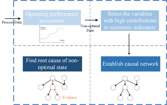
Due to environmental fluctuations, the operating performance of complex industrial processes may deteriorate and affect economic benefits. In order to obtain maximal economic benefits, operating performance assessment is a novel focus. Therefore, this paper proposes a whole framework from operating performance assessment to nonoptimal cause identification based on partial-least-squares-based Granger causality analysis (PLS-GC) and Bayesian networks (BNs). The proposed method has three main contributions. First, a multiblock operating performance assessment model is established to correspondingly extract economic-related information and dynamic information. Then, a Bayesian network structure is established by PLS-GC that excludes the strong coupling of variables and simplifies the network structure. Lastly, nonoptimal root cause and and nonoptimal transmission path are identified by Bayesian inference. The effectiveness of the proposed method was verified on Benchmark Simulation Model 1.

Graphical Abstract

1. Introduction

Along with the continuous development of industrial technology, the requirements of modern industry are increasing. Process monitoring is no longer limited to fault detection, and the operating state of industrial process with low economic benefits needs detection. Even though nonoptimal operating state is not as serious as faults, it still affects the economic benefits of the process. In order to ensure the economic benefits of processes, a nonoptimal operating state needs to be immediately detected. Due to production environment changes, equipment aging, parameter drift, etc., industrial processes may deviate from the optimal state, showing multimode characteristics. Therefore, operating performance assessment is increasingly important, and it divides operating conditions into an optimal and multiple nonoptimal grades according to the economic benefits of the corresponding states. Due to the high complexity of industry processes, it is difficult to establish a model according to the process mechanism alone. Data-driven methods are attracting increasing attention [1,2], and many basic data-driven methods were applied in performance assessment, such as principal component analysis (PCA) [3]. Then, with the enlargement of data, complex characteristics in these data have gradually attracted the attention of researchers. For example, in consideration of the nonlinearity of the process, Liu et al. [4] put forward a method based on kernel total projection to latent structures and kernel-optimality-related variations. Considering the existence of process noise and outliers, Chu et al. [5] proposed a total robust kernel projection to the latent structure algorithm. The above methods aimed at single-process characteristic problems, while operating performance assessment was oriented to complex industrial systems with multiple process characteristics. In order to evaluate performance in a multiple-characteristic process, the whole process can be divided into multiple blocks [4,6,7,8].
In addition, in order to improve the comprehensive production profit, when the process enters nonoptimal state, operators need to make adjustments according to different nonoptimal causes. The process of nonoptimal cause identification is similar to fault diagnosis. Venkatasubramanian et al. [9] classified fault diagnosis methods into qualitative-model-, quantitative-model-, and process-history-based methods. The most popular quantitative-model-based method is contribution plots [10], which calculates the influence of each variable to the statistics to identify the cause variable. Because the basic contribution-plot method suffers from the fault smearing effect, Cheng et al. [11] proposed a moving average residual difference reconstruction contribution plot to identify the root cause in wastewater treatment processes. In addition, due to the existence of dynamic characteristics, Li et al. [12] proposed a dynamic time-warping-based causality analysis method to perform root diagnosis for nonstanionary faults. However, these methods can only find the most related variable to the fault. Detecting the cause–effect relationship between variables is needed, on which many studies were conducted [13]. The most prevalent measure is Granger causality analysis (GC) [14]. Granger causality analysis was initially used in the time series of economic studies, with the continuous research of other scholars, it has shown promise in many other fields [15,16]. Because GC is only useful in linear processes, aiming at nonstationarity and nonlinearity in industrial processes, Chen et al. [17] embedded Gaussian process regression into a multivariate Granger causality framework. Transfer entropy can also effectively solve nonlinear problems. Lindner et al. [18] proposed a method to find the optimal parameters of transfer entropy by the dynamism of the process. In addition to the above methods, Bayesian networks are also widely used in root-cause identification [19] because they have the structure of directed acyclic graph (DAG), which is very helpful in the identification of fault transmission paths. However, it is difficult to construct Bayesian networks in a complex industrial process. Therefore, the hierarchical approach was used in many studies. Chen et al. [20] constructed a hierarchical Bayesian network structure, and built a statistical index for process monitoring and fault diagnosis. Suresh et al. [21] proposed a hierarchical approach to capture cyclic and noncyclic features.
Although the above methods are effective, they also come with defects. For example, GC can only be used for linear systems, transfer entropy is sensitive to parameters, and BN is only suitable for directed acyclic graphs (DAGs). Chemical industrial processes are composed of a large number of process variables with high correlation, so the causal structure is probably not acyclic. Therefore, in this paper, contribution plots are used to select some variables before constructing the causal network, which simplifies the calculation and reduces the possibility of generating cynic structures. Then, considering the strong coupling characteristics between process variables, partial least squares (PLS) algorithm [22,23] is incorporated into the regression operation of GC to eliminate the influence of the correlation between variables. This operation also reduces the number of detected causal relationships, further reducing the possibility of generating cynic structures in causal network. Lastly, on the basis of the causal structure established by PLS-GC, the root cause can be identified through BN. The main contributions of this paper are summarized as follows:
(1)
A complete framework from operating performance assessment to nonoptimal cause identification is established. Process data are divided into multiple operating grades, so that field operators can detect operational states with poor economic benefits and adjust them in time.
(2)
In order to establish a causality network, contribution plots and Granger causality analysis are used in this paper, which avoid the NP-hard problem of searching for the causal network structure.
(3)
PLS-GC method is proposed to replace simple GC, which can remove false causalities caused by variable coupling and reduce the possibility of generating a cyclic structure in causal networks.
(4)
Through Bayesian network inference, both nonoptimal causes can be identified, and the transmission path of nonoptimal causes can be obtained.
The rest of this paper is organized as follows. In Section 2, the basic concepts of GC and BN are introduced. Subsequently, Section 3 presents an operating performance assessment strategy and the nonoptimal root-cause identification method. In Section 4, the effectiveness of the method is proved on the basis of an experiment on Benchmark Simulation Model 1. Section 5 concludes this work.

2. Preliminaries

2.1. Granger Causality Analysis

In the definition of GC [14], if a variable X 1 causes another variable X 2 , knowing the past of X 1 is beneficial in predicting X 2 . Consider two time series, X 1 and X 2 . If the prediction of X 1 considering the past information of X 1 and X 2 is more accurate than that only considering the past information of X 1 , according to the definition of GC, X 2 is considered to be the Granger cause of X 1 .
An autoregression model that contains only the past information of X 1 is constructed as follows:
X 1 ( t ) = a 0 + i = 1 p a i X 1 ( t i ) + ε 1 ,
If the past information of X 1 and X 2 is taken into consideration, the union-regression model is defined as follows:
X 1 ( t ) = b 0 + i = 1 p a i X 1 ( t i ) + j = 1 q b j X 2 ( t j ) + ε 12 ,
where p and q are the lags of X 1 and X 2 , respectively, which can be determined by the Akaike or Bayesian information criterion. a 0 , b 0 , a i and b j denote the regression coefficient. ε 1 ( t ) and ε 12 represent the autoregressive residual of X 1 and the union-regression residual of X 1 and X 2 , respectively.
According to the definition of GC, prediction accuracy is expressed by the variance of residuals. Granger indicators from X 1 to X 2 can be constructed as follows:
F X 2 X 1 = ln var ε 1 var ε 12 .
If F X 2 X 1 > 0 , X 2 can be considered the Granger cause of X 1 , and if F X 2 X 1 0 , there is no causal relationship between X 1 and X 2 .
Then, the statistical significance of F X 2 X 1 can be tested by F statistics:
F statistic = RS S A R RS S U R / p RS S A R / N 2 p 1 F p , N 2 p 1 ,
where RS S A R and RS S U R represent the residual sum of squares of autoregression and union-regression respectively. N denotes the number of samples.
There are many variables in the actual industrial process. In order to solve multivariate problems, researchers extended GC to multivariate conditional Granger causality analysis. The past information of other variables is introduced into autoregression and union regression in order to reduce their interference on causal analysis between X 1 and X 2 . The autoregression and union-regression models are calculated as follows:
X 1 ( t ) = a 0 + i = 1 p a i 1 X 1 ( t i ) + j = 3 m i = 1 p a i j X j ( t i ) + ε 1 ,
X 1 ( t ) = b 0 + i = 1 p a i 1 X 1 ( t i ) + i = 1 p a i 2 X 2 ( t i ) + j = 3 m i = 1 p a i j X 2 ( t i ) + ε 12 ,
where m is the number of variables, a i j represents regression coefficient of variable j when time delay is i. Similar to GC, the causal relationship between variables X 1 and X 2 can also be analyzed by F statistics.

2.2. Bayesian Network

Bayesian network [24] is a direct graphical model composed by nodes and directed edges. Through a directed acyclic graph, the conditional dependencies of a set of variables are presented [25]. In the last few decades, BN has been widely used in fault diagnosis [26,27,28]. Because BN is a model based on a causal graph, it is suitable for root identification. Fault transmission paths can be obtained through the causal relationship structure of BN.

2.2.1. Fundamentals of Bayesian Networks

BN consists of a qualitative and a quantitative part. The qualitative part is the Bayesian network structure, and the quantitative part is the conditional probability table (CPT) that represents dependencies between variables. The structure of BN can be expressed as follows:
B N = G , P ,
where G represents the network structure, and P represents network parameters. G = V , E , where V denotes the variable set, and E denotes an unidirectional arc set that describes dependencies between variables. In chemical processes with recycling, we can use duplicate dummy variables [29] to remove the circular structure, as shown in Figure 1. Node A is divided into two nodes so as to construct a directed acyclic graph.
Considering n nodes of BN X = X 1 , X 2 , , X n , the general expression of Bayesian networks is as follows:
P ( X 1 , X 2 , , X n ) = i = 1 n P ( X i | p a ( X i ) ) ,
where p a ( X i ) denotes the parent nodes of X i , P ( X 1 , X 2 , , X n ) is joint probability distribution.
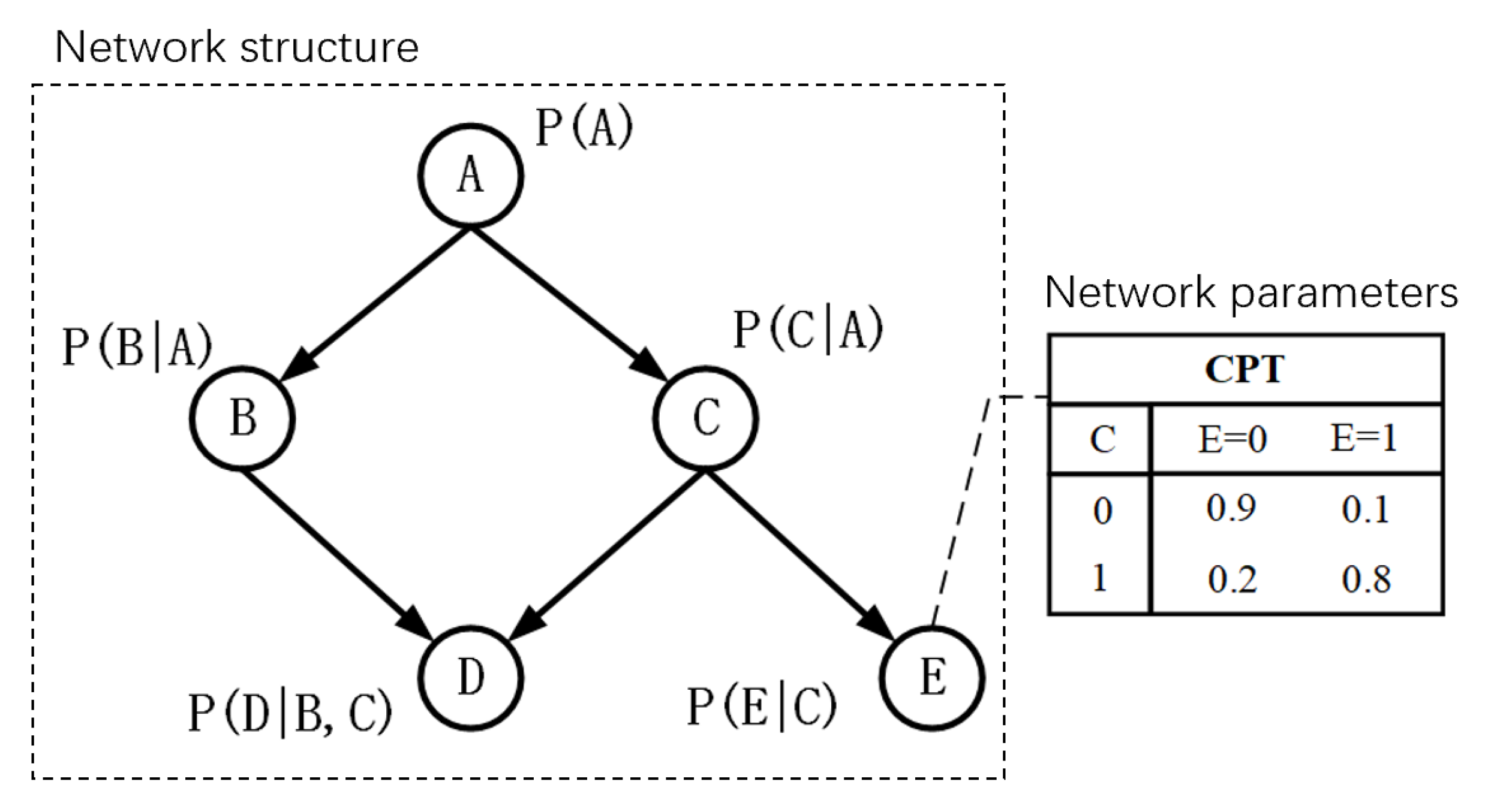
Network parameters consist of prior and conditional probabilities. Prior probabilities are usually calculated according to expert knowledge observations. Conditional probabilities are usually contained in CPT. For instance, a simple Bayesian network model is given in Figure 2. On the left is a Bayesian network structure, and on the right is the CPT of node E, where E = 0 represents that probability E does not occur. Because C is a parent node of E, whether C occurs should also be taken into consideration in the calculation.

2.2.2. Inference Algorithm of Bayesian Network

BN can perform backward inference through the Bayes theorem. The BN inference problem is NP-hard, and many scholars conducted indepth research and achieved extensive progress [30,31]. In general, inference algorithms can be divided into two categories: exact and approximate inference. Exact inference, such as junction trees, can obtain the exact probability value of each node, while approximate inference uses statistical methods to compute approximate probabilities. Next, two exact inference algorithms are introduced: variable elimination and belief propagation.
The variable elimination algorithm is a basic exact inference algorithm. The core idea is dynamic programming. Conditional independence is used to reduce calculation. Through changing the operational order of summation and product, the elimination order calculating joint probability is changed. Figure 3a is an example, and X 1 , X 2 , X 3 , X 4 , X 5 are nodes in BN. If our target is calculating marginal probability P ( X 5 ) , X 1 , X 2 , X 3 , X 4 should be eliminated.
P ( X 5 ) = X 4 X 3 X 2 X 1 P ( X 1 , X 2 , X 3 , X 4 , X 5 ) .
According to the relationships between variables, it can be rewritten as:
P ( X 5 ) = X 4 X 3 X 2 X 1 P ( X 1 ) P ( X 2 | X 1 ) P ( X 3 | X 2 ) P ( X 4 | X 3 ) P ( X 5 | X 3 ) .
If we change the calculation order, there is
P ( X 5 ) = X 3 P ( X 5 | X 3 ) X 4 P ( X 4 | X 3 ) X 2 P ( X 3 | X 2 ) X 1 P ( X 1 ) P ( X 2 | X 1 ) .
Then, m i j ( X j ) is used to represent the intermediate results, in which i means it is the result of summing X i and j represents the other variables in this item. According to this idea, the above formula can be transformed into P ( X 5 ) = m 35 ( X 5 ) , which is only related to X 5 . The calculation is simplified.
A belief propagation exact inference algorithm is proposed on the basis of a variable elimination algorithm to overcome redundant computation In belief propagation algorithms, and summation operation is a process of message passing as shown in Figure 3b. The process of message passing comprises two steps. First, a root node is assigned, and messages are delivered to the root node from all leaf nodes until the root node receives messages from all adjacent nodes. Then, the message is delivered from the root node to leaf nodes until all leaf nodes receive messages. Because each variable node receives information from adjacent nodes, we can calculate the edge probability distribution of each variable.

3. Method Development

In order to obtain better economic benefits, we need to monitor the operational process so as to detect nonoptimal operation states in time. When the operating process is nonoptimal, it is necessary to identify its root cause for further adjustment. Complex industrial processes are composed of a large number of high coupling process variables, many of which may change during nonoptimal grades, but we need to find out which variable causes the change in others, that is, the root cause of nonoptimal grades. Therefore, a framework from operating performance assessment to nonoptimal cause identification is established in this section.

3.1. Establishment of Operating Optimality Assessment Model

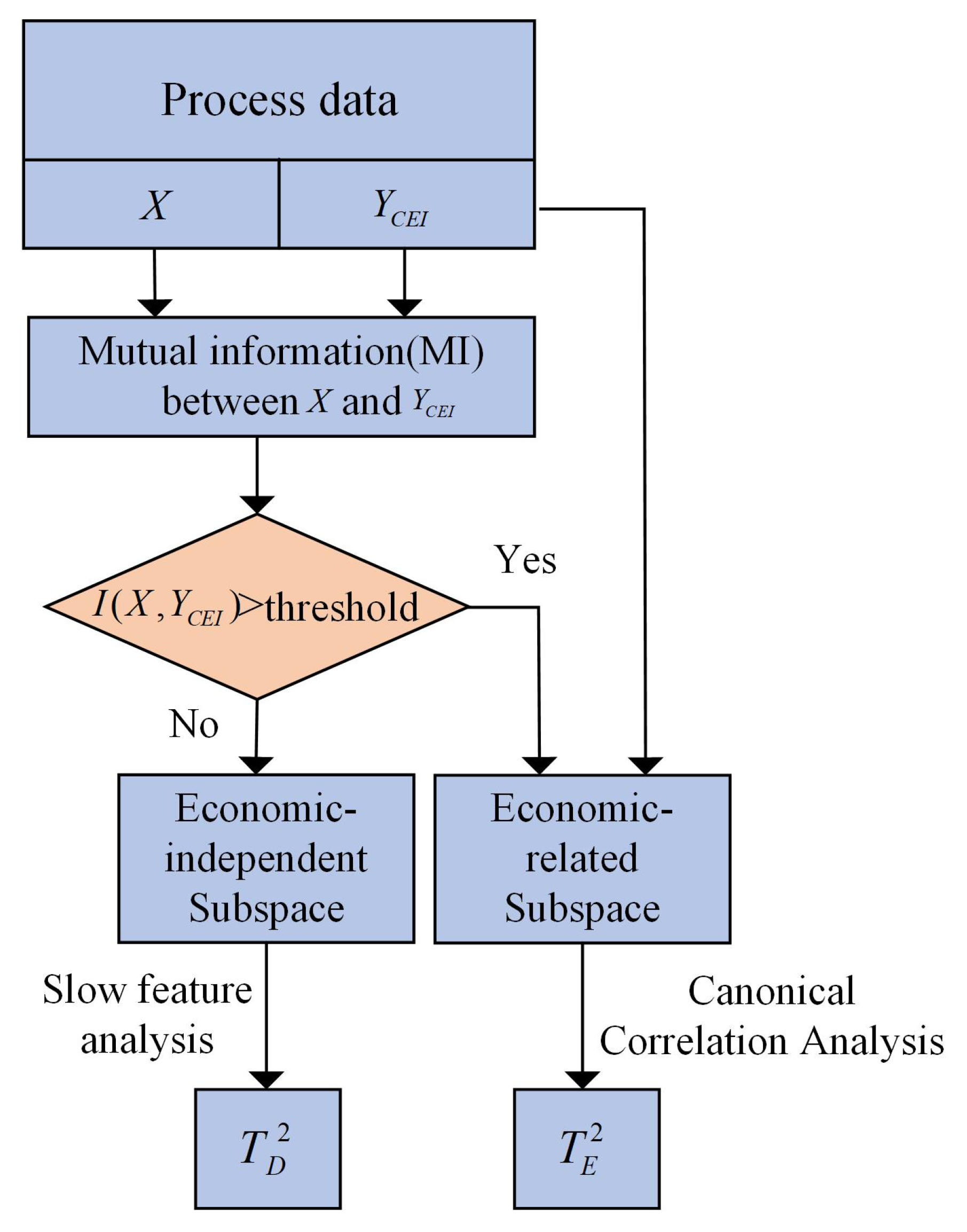
Inspired by the multiblock technique, mutual information is used to divide process variables into two blocks. Then, dynamic and economic relevant information is extracted from two blocks. The process of performance assessment is shown as Figure 4.
First, training process data are divided into several operating performance grades according to the comprehensive economic indicator (CEI). Here, we assumed that process data were from three different performance grades. Then, the performance grade with the highest economic benefit was labeled as good, and the two other grades are labeled as medium or poor, and both are considered to be nonoptimal. According to the correlation between variables and economic indicators, we divided process variables into economic-related (ERS) and economic-independent (EIS) subspaces. Correlation is measured by mutual information (MI). MI is a measure of interdependence between random variables [32].
I ( X , Y ) = H ( X ) H ( X | Y ) ,
where H ( X ) represents the information entropy of X and H ( X | Y ) represents conditional entropy, which means the uncertainty of X while Y is known. From the perspective of probability, MI is represented as
I ( X , Y ) = y Y x X p ( x , y ) log ( p ( x , y ) p ( x ) p ( y ) ) ,
where p ( x , y ) denotes joint probability distribution, and p ( x ) , p ( y ) denotes marginal probability distribution. Offline training data from one performance grade are denoted as X = x 1 , x 2 , , x m T R m × n , where m represents the number of process variables and n represents the number of samples. The corresponding economic indicator (CEI) is represented as y CEI R 1 × n . According to the mutual information between each variable and economic index, process variables are divided into two subspaces: economic subspace X E and economic-independent subspace X D . ERS contains more directly related information to the economic indicator, so canonical correlation analysis (CCA) is used to extract economic information in ERS and construct T D 2 statistics [33]. Although EIS contains less economic related information, it covers a lot of process variation information. Therefore, slow feature analysis (SFA) [34] is used to extract dynamic features and construct T E 2 statistics. Then, for an input sample x k with statistics T l 2 , the probability that x k belongs to operating performance grade C l is expressed as:
Pr [ C l | T l 2 ( x k ) ] = Pr [ T l 2 ( x k ) | C l ] Pr ( C l ) Pr [ T l 2 ( x k ) | C l ] Pr ( C l ) + Pr [ T ¯ l 2 ( x k ) | C ¯ l ] Pr ( C ¯ l ) ,
where P r ( C 1 ) is the probability that the current sample belongs to grade C l , and P r ( C ¯ l ) is the prior probability that the current sample belongs to other grades. Pr [ T l 2 ( x k ) | C l ] and Pr [ T ¯ l 2 ( x k ) | C ¯ l ] are likelihoods calculated as:
Pr [ T l 2 ( x k ) | C l ] = exp ( T l 2 ( x k ) T ¯ l 2 ) ,
Pr [ T l 2 ( x k ) | C ¯ l ] = exp ( T ¯ l 2 ( x k ) T l 2 ) ,
Lastly, according to Bayesian inference, global probability can be obtained [35], which is also the similarity index of x k to grade C l :
S I l ( x k ) = Pr [ T l 2 ( x k ) | C l ] Pr [ C l | T l 2 ( x k ) ] D + Pr [ T l 2 ( x k ) | C l ] Pr [ C l | T l 2 ( x k ) ] E Pr [ T l 2 ( x k ) | C l ] D + Pr [ T l 2 ( x k ) | C l ] E ,
which combines the statistics of the two subspaces.

3.2. Nonoptimal Root Cause Identification

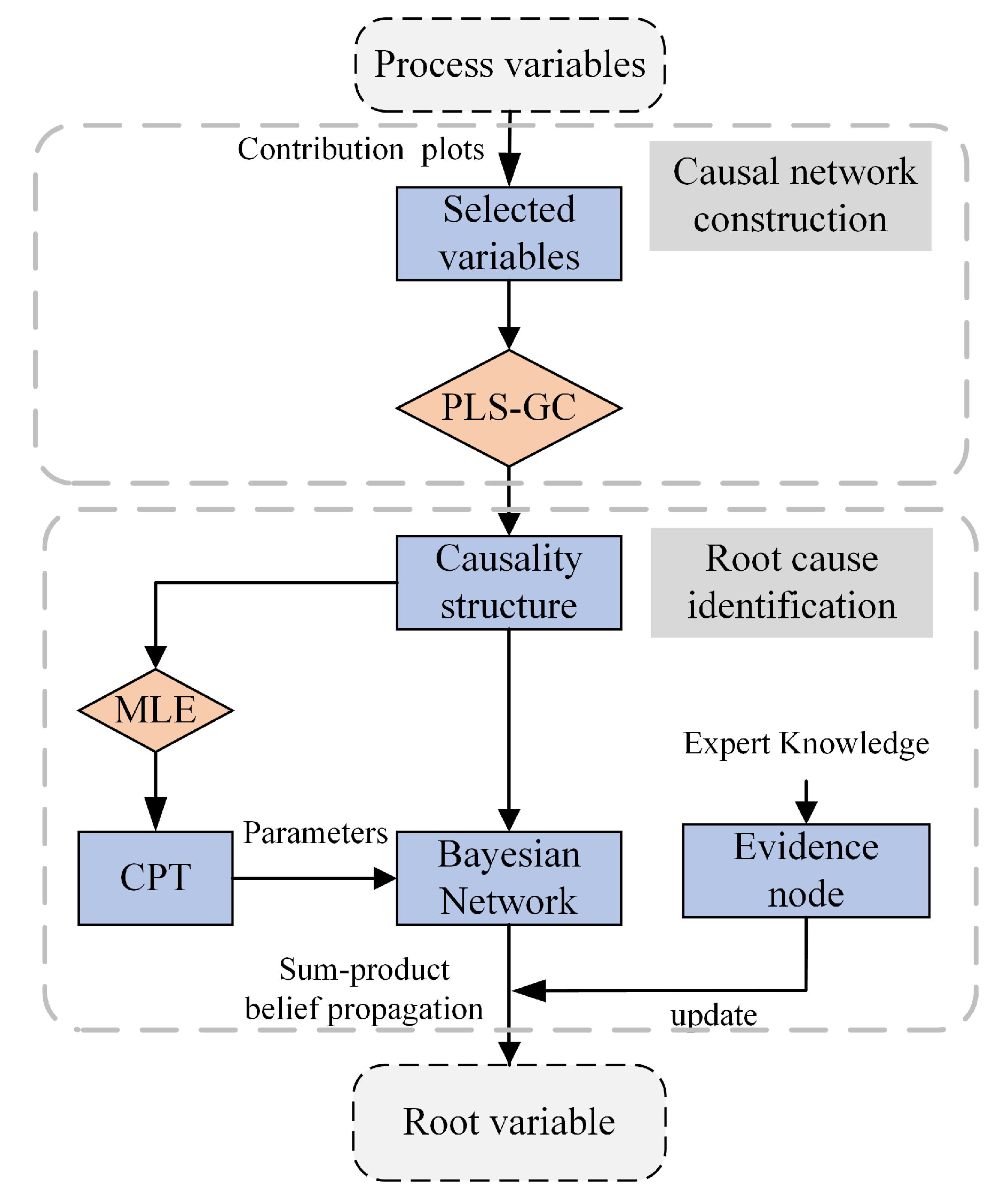
In order to maintain the best performance of an operating process, operators must know the cause of nonoptimal states. In this section, a data-based cause identification method is proposed. A system block diagram is given in Figure 5. Nonoptimal root cause identification comprises two steps. First, a causal network is constructed. Then, the evidence node is determined, and the nonoptimal root cause is identified.

3.2.1. Causal Network Establishment

First, the network structure need to be constructed. Because chemical processes are composed of complex structures, we conducted the preliminary screening of variables with contribution plots and selected the candidate variables most related to the economic indicators to reduce calculation. The PCA contribution plot method is simple and intuitive, and was widely studied in fault diagnosis [4,10].
Assume that map matrix P of PCA was obtained. The T 2 statistic of sample x is:
T 2 = x T P S 1 P T x ,
where S is covariance matrix of training data. Then, the contribution rate can be calculated as:
C i T 2 = ξ i T P S 1 P 1 2 x 2 ,
where ξ i is a unit column vector. If the contribution rate is above average, the corresponding process variable is included in the candidate variable set.
After selecting the candidate variable set, the network structure can be constructed with PLS-GC. Because multivariate conditional Granger causality analysis only uses the least-squares method to construct regression models, it is easy to mistakenly regard correlation between variables as a causal relationship, which leads to wrong results.
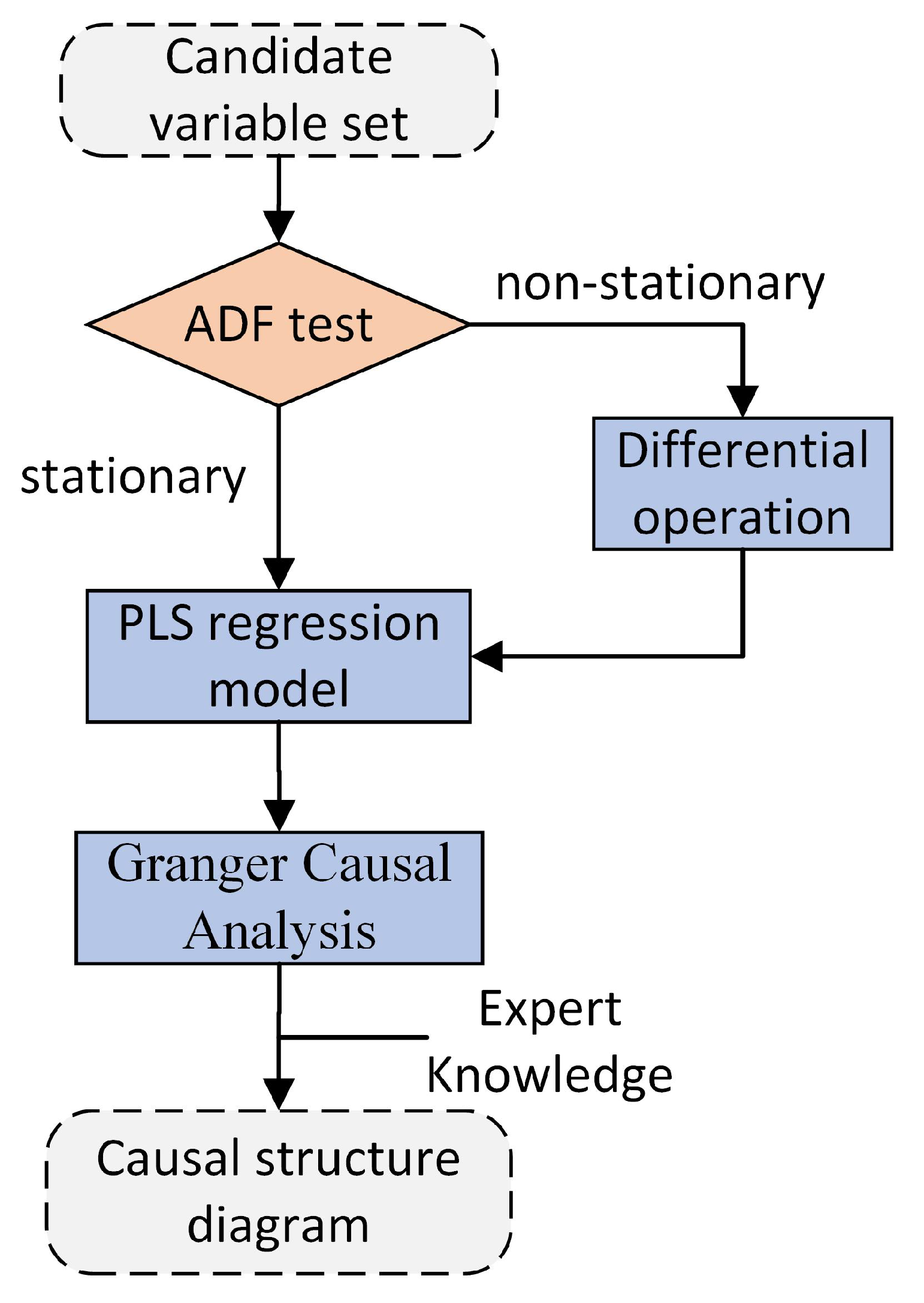
Therefore, PLS is used to replace the autoregression model in GC, which can effectively deal with union correlation in multiple variables, and construct a network structure with clear causality relationships. Because GC requires variables to be stationary, we need to ensure that candidate variables are all stationary. Generally, stationarity is tested by whether there is a unit root in the time series. Therefore, the augmented Dickey–Fuller (ADF) unit root test [36] was conducted in advance. Differential operation is performed on nonstationary variables.
The specific process of network construction is given in Figure 6:
  • Candidate variables are selected for causality structure construction by PCA contribution plots.
  • ADF test is conducted to ensure that all variables are stationary
  • For all stationary variables x 1 , x 2 , , x n , we selected two variables x i and x j , i , j { 1 , , n } , establish autoregression model and union-regression model by PLS and calculate F statistics. If p value of F statistic is in the confidence interval β , there is a causal relationship from x i to x j . Such a causality test is conducted on each pair of variables in turn.
  • A causal network structure is constructed and adjusted according to expert knowledge.

3.2.2. Nonoptimal Cause Identification

Before nonoptimal cause identification, we need to calculate the network parameters, that is, nonoptimal and conditional probabilities. Nonoptimal probability is generally determined by parameter learning with historical data. Since process data were known, maximum likelihood estimation (MLE) could be used to learn the parameters of the Bayesian network.
MLE is the most popular parameter learning method at present, which is effective and suitable for large-scale datasets. The whole process contains optimal and nonoptimal processes. Data in optimal state were considered within the threshold range, and data in nonoptimal state were considered outside the threshold range. The threshold range of each variable can be determined by kernel density estimation [37], so that each variable can be divided into two states.
Given a sample set containing p variables, D = u 1 , u 2 , , u p , each of which contains N samples, u i = u i 1 , u i 2 , , u i N , i = 1 , 2 , , p , MLE requires sample set D to satisfy independent identically distributed hypothesis, so the joint probability can be written as follows:
P u 1 , u 2 , , u p | θ = i = 1 p P u i | θ = L Θ | D ,
where L Θ | D is the likelihood function of P D | θ . If variable u i comprises r i values, and its parent node π u i is composed of q i different combination values, then the unknown parameters can be expressed as Θ = θ i j k | i = 1 , , p ; j = 1 , , q i , k = 1 , r i : where θ i j k represents the probability of u i being k when the parent node is j. In order to find the parameters that satisfy the following condition:
Θ * = arg max Θ L Θ | D ,
where the logarithmic likelihood function L Θ | D can be expressed as:
ln L Θ | D = ln κ = 1 p P u κ | θ = i = 1 N j = 1 q i k = 1 r i m i j k ln θ i j k ,
where m i j k is the number of u i in D with the value k and parent nodes with the value j. Then calculate maximum likelihood values and obtain the CPT of each node.
After determining the network structure and parameters of BN, network inference can be carried out. First, evidence nodes are determined according to expert knowledge and contribution plots. Second, the posterior probability of each variable is calculated with sum-product belief propagation, and the CPT of Bayesian network is updated. Detailed steps of BN nonoptimal cause identification are given as follows:
  • On the basis of PCA contribution plots, select the candidate variable set.
  • Construct the network structure on the basis of PLS-GC.
  • Calculate the conditional probability and obtain CPT.
  • Determine evidence variable according to industry field experience and contribution plots. Among the resulting variables in the causal network, the one with the largest contribution is the evidence node. Then, update the network parameters with the belief propagation method and identify the root nonoptimal variable.

4. Results and Discussion

4.1. Process Description

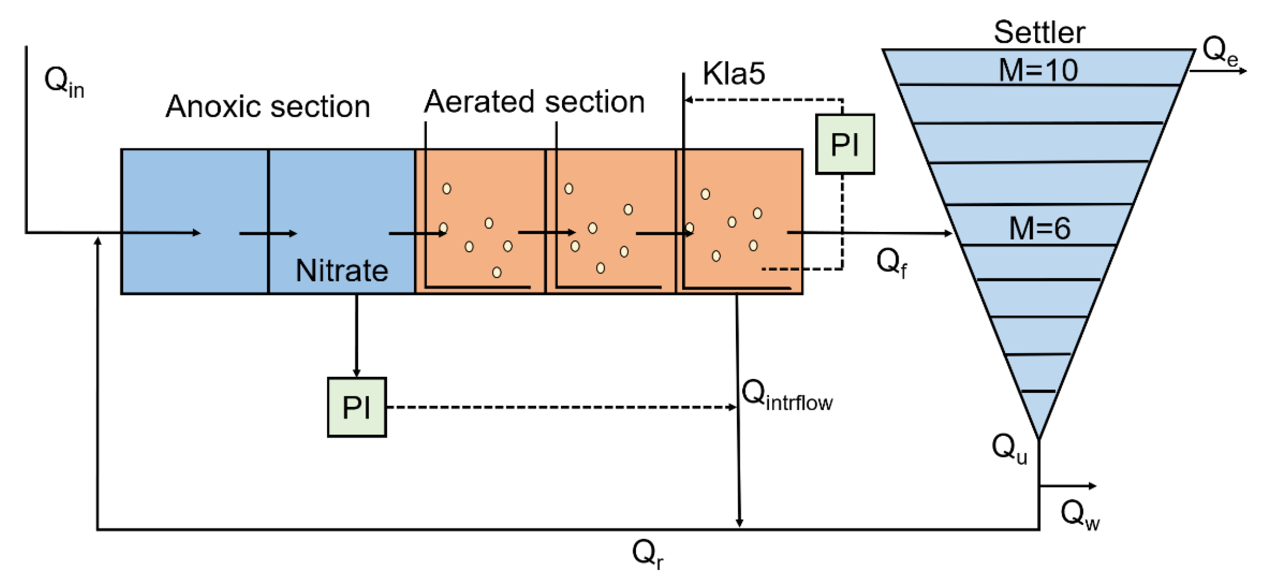
Benchmark Simulation Model 1 (BSM1) was developed by the International Water Quality Association and the European Cooperation in the field of Scientific and Technical Research, and was widely used in control simulation and performance evaluation of wastewater treatment process. Activated sludge model ASM1 and double index secondary sedimentation tank model were used to simulate the actual wastewater treatment process. The research object of BSM1 is predenitrification biological nitrogen removal technology, which is composed of five activated sludge reaction units and a secondary sedimentation tank. The structure diagram of the model is shown in Figure 7 [38]. The activated sludge reactor comprises two anoxic tanks and three aerobic tanks. Part of the water from the reaction tank flows into the sixth layer of the secondary sedimentation tank, wastewater is discharged from the tenth layer after sedimentation, and the excess sludge is discharged from the bottom layer.
In order to evaluate the performance of BSM1 under different operating conditions, the model provides an overall cost index (OCI) [39], which reflects the overall cost of the whole process during operation and is calculated as follows:
OCI = AE + rPE + 5 × SP + 3 × EC + ME ,
where AE is aeration energy consumption, PE is pump energy consumption, SP is sludge production, EC is external carbon source consumption, and ME is mixing energy consumption.

4.2. Data Preparation

In order to verify the effectiveness of the proposed method, two training datasets with three performance grades were simulated on BSM1. The dissolved oxygen concentration of tank 5 was changed in Dataset 1, which was set to 2, 3, and 4 gCOD/m 3 , respectively. Nitrate and nitrite concentration of tank 2 was changed in Dataset 2, which was set to 1, 1.5, and 2 gN/m 3 . According to the OCI of the training data, the operational state with higher overall cost was of poor grade. In this way, training data were divided into three grades (good, medium, poor).
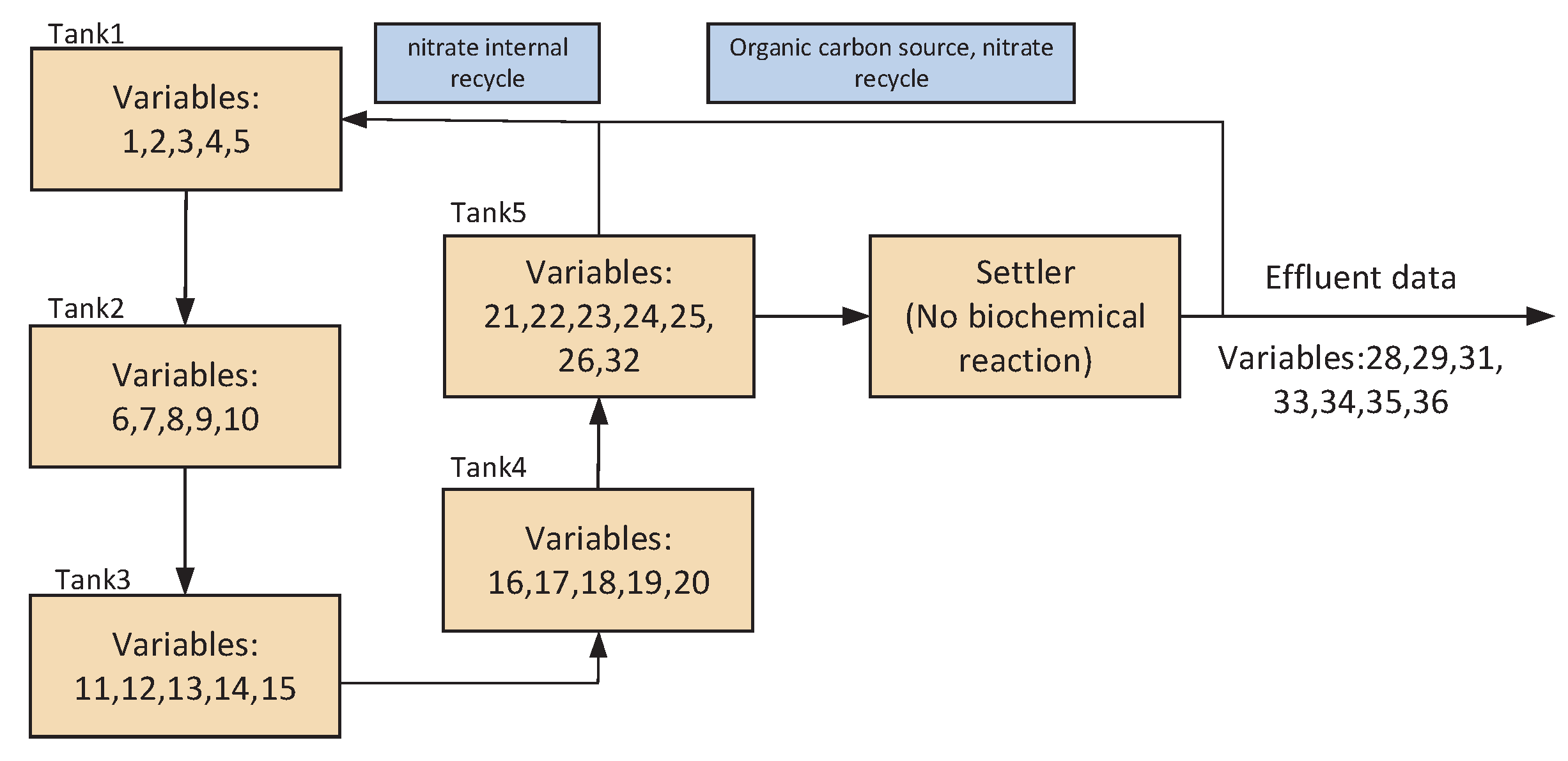
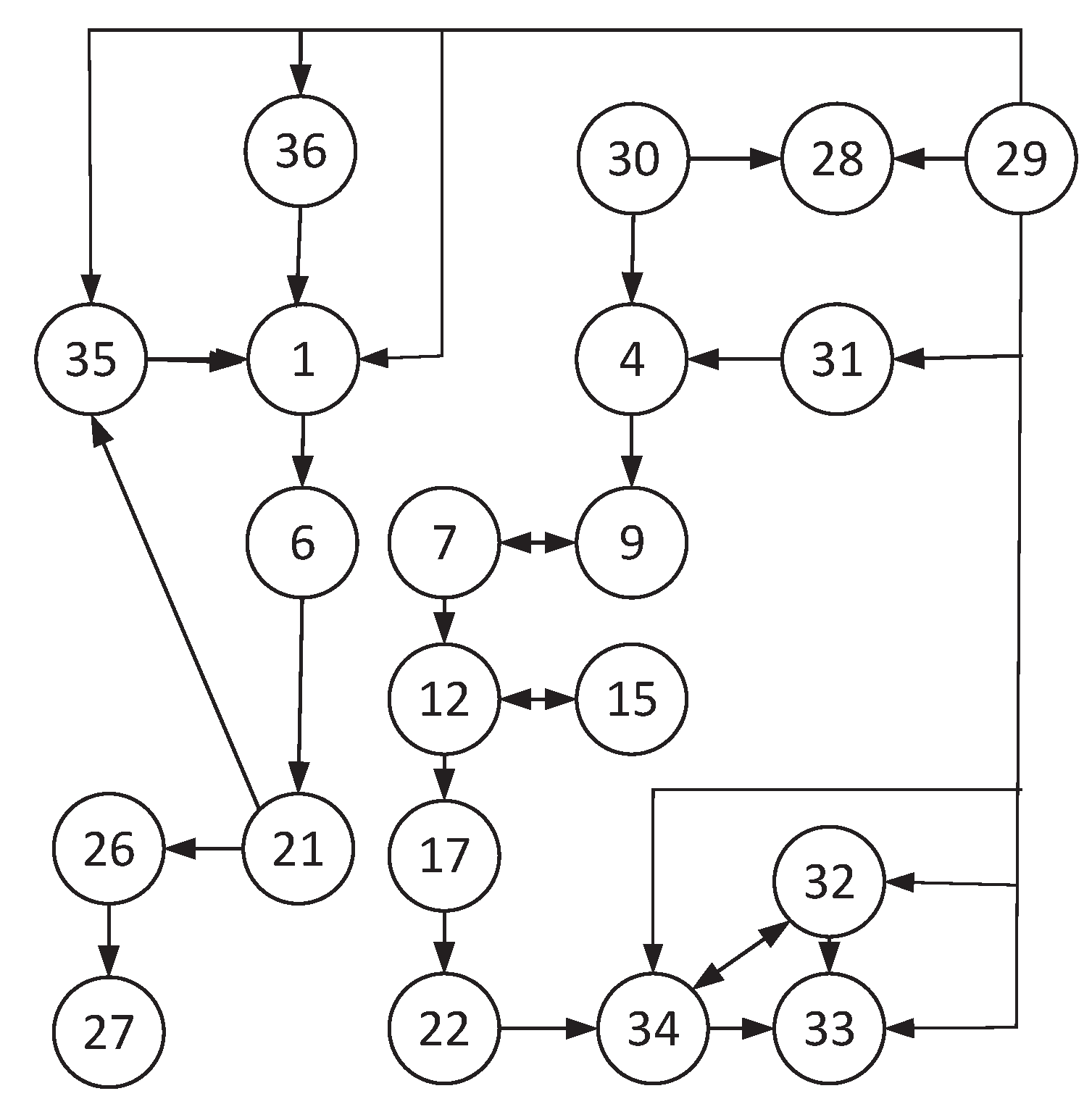
All experiments were carried out on MATLAB. Process variables of training data are given in Table 1. According to the structural schematic diagram in Figure 7, variable location and relationships are given in Figure 8. In order to render the model more realistic, a delay device with a delay factor of 0.001 was added after the first reaction tank of model BSM1.

4.3. Operating Performance Assessment and Nonoptimal Cause Identification

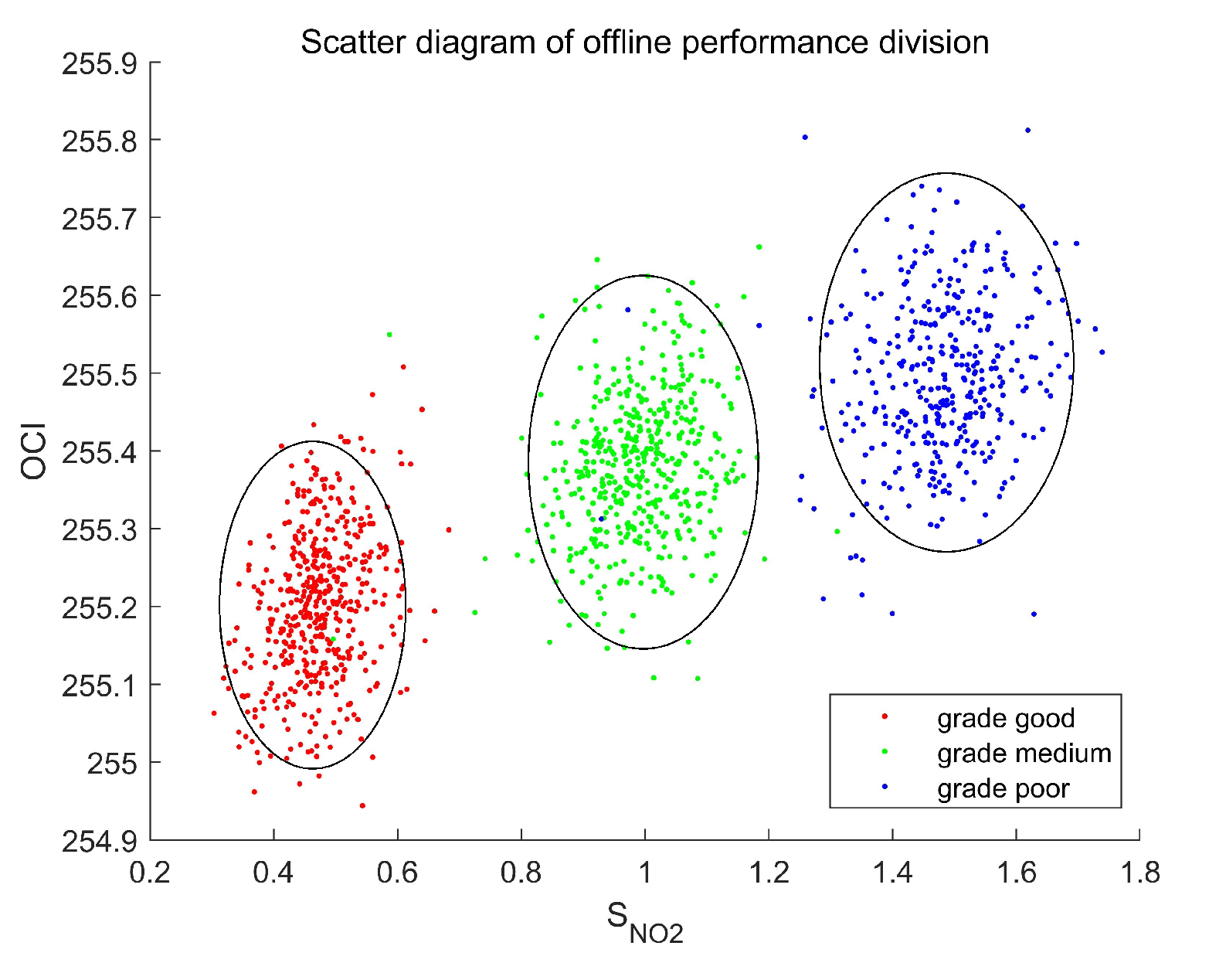
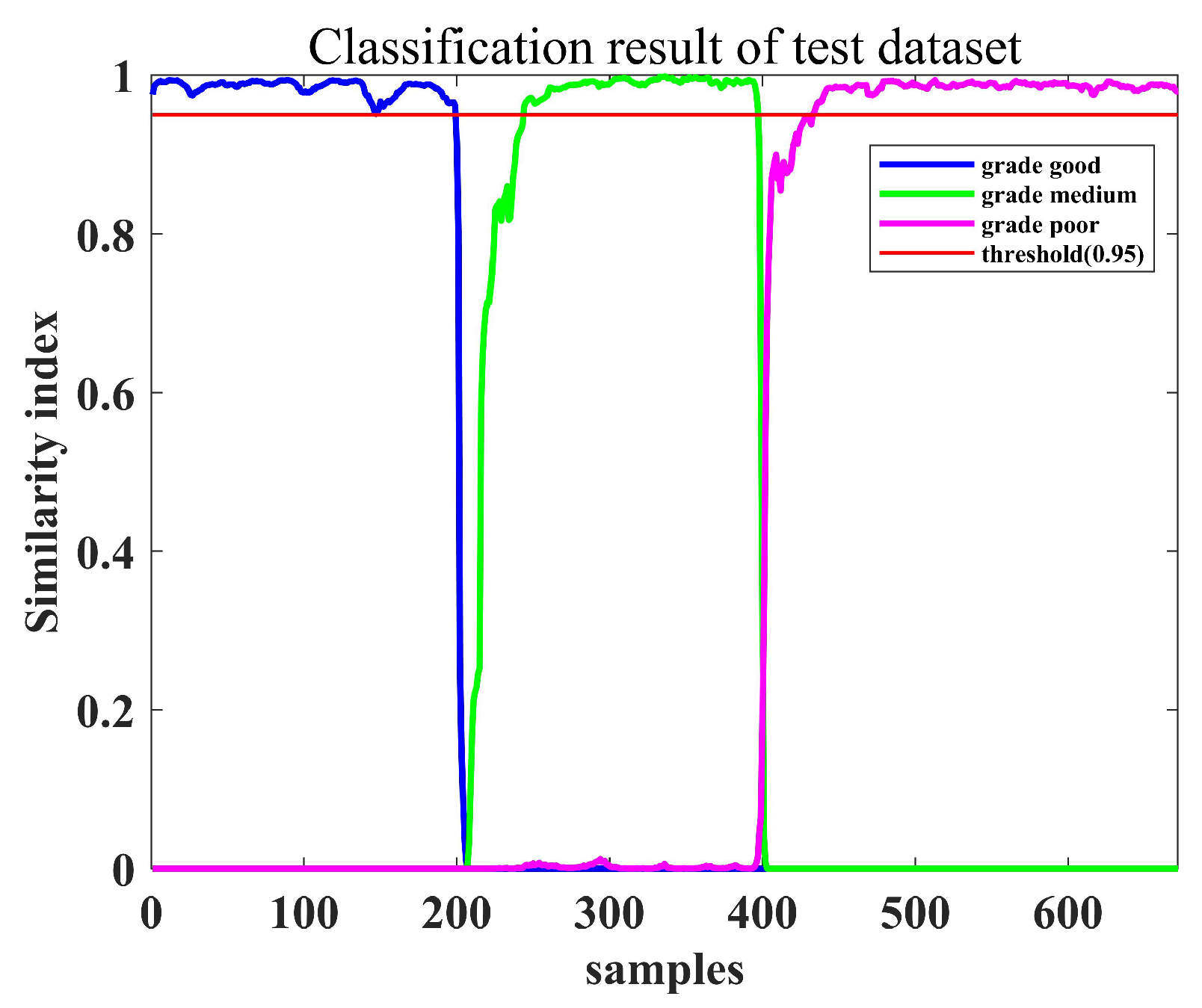
First, performance grades were divided according to the average OCI of each states as shown in Figure 9. The operating state with minimal OCI was considered to be of good grade. Then, the mutual information between each variable was calculated, and process variables were divided into two subspaces. Parameters are set as follows: window width, 10; threshold of mutual information, 0.3; threshold of similarity index, 0.95. The similarity index of the test dataset is given in Figure 10. In order to prove the effectiveness of this method, we conducted a comparative experiment on a test dataset. In this test dataset, the grade of samples 1–192 was good, that of 194–385 was medium, and that of 386–672 was poor. Then, accuracy was calculated according to the known label of the test dataset. Table 2 shows that CCA-SFA was more effective than CCA or SFA alone.
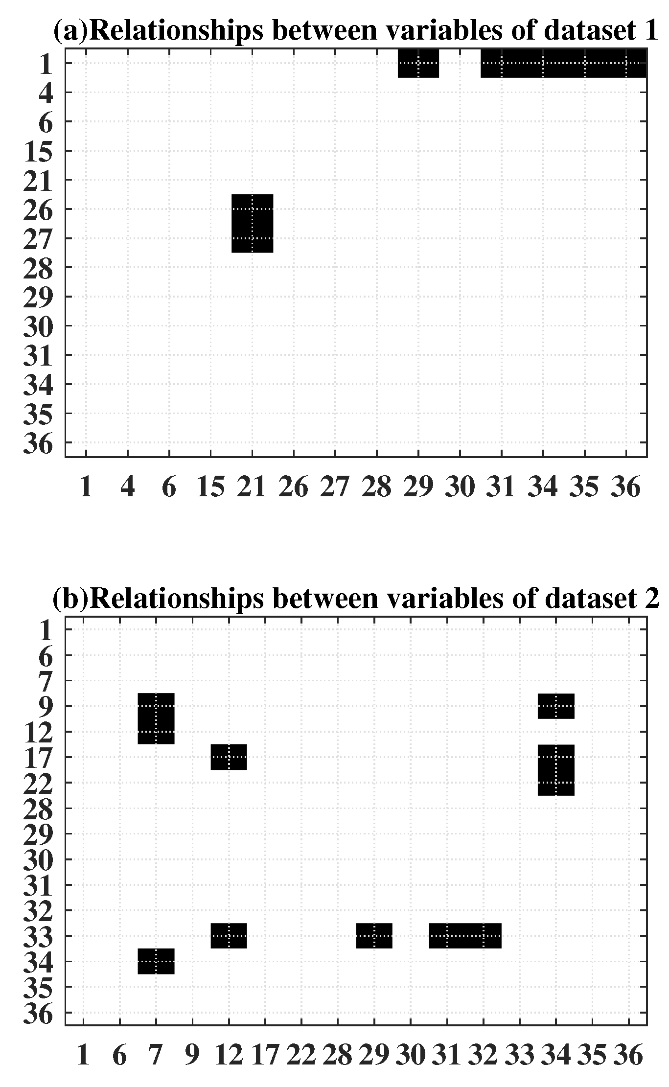
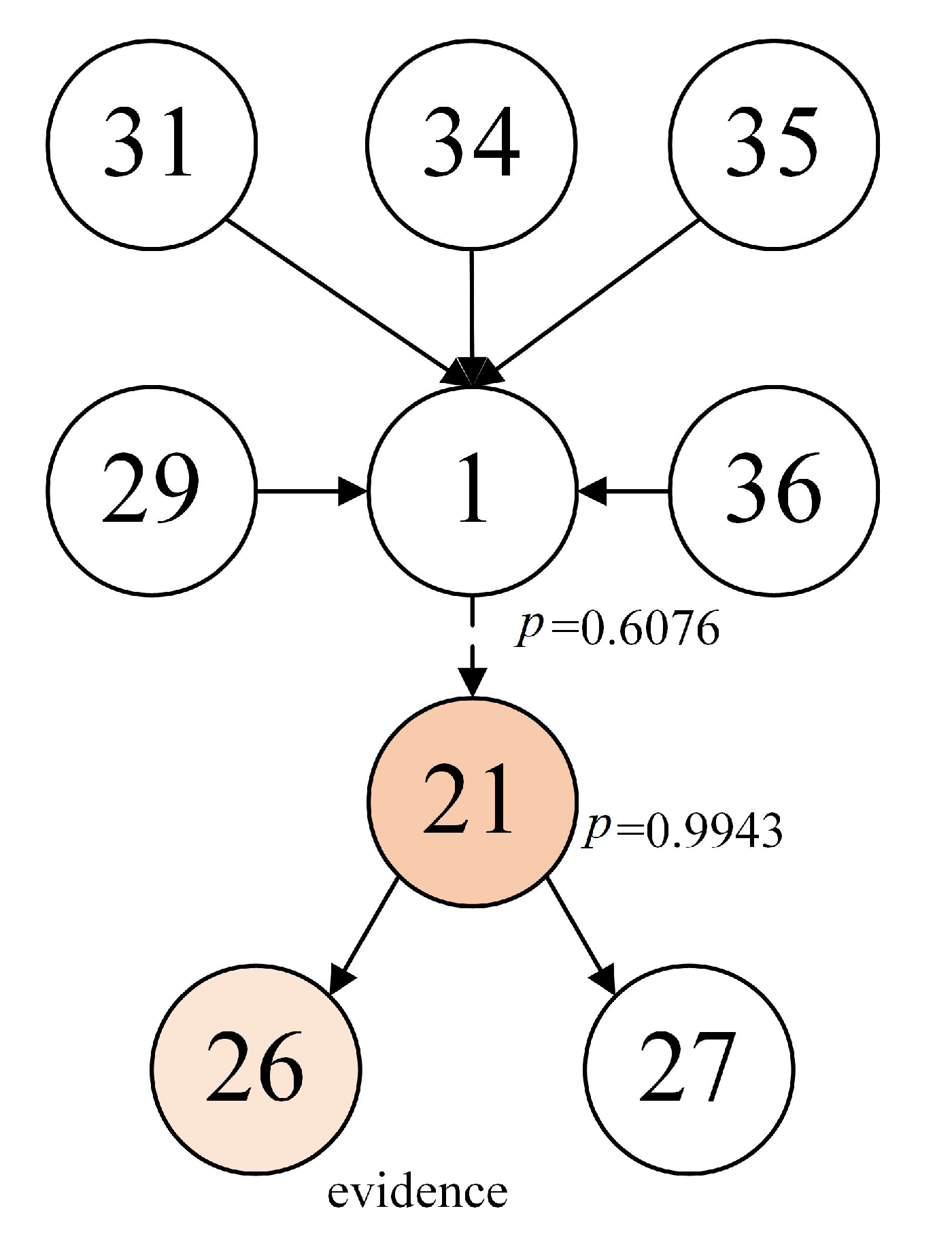
In these three operating grades, grades of medium and grade poor were both considered to be nonoptimal. In follow-up experiments, the medium grade was taken as an example for nonoptimal cause identification. Results of contribution plots are given in Figure 11. The red line represents the average contribution rate, and we selected above average variables as the candidate sets. According to Figure 11, variable set 1, 4, 6, 15, 21, 26, 27, 28, 29, 30, 33, 34, 35 was selected for Dataset 1, and variable set 1, 6, 7, 9, 12, 17, 22, 28, 29, 30, 31, 32, 33, 34, 35, 36 was selected for Dataset 2. Then, the network structure diagram was established with PLS-GC, delay factors were set to 2, and the number of hidden variables in PLS was set to 6. The results of the two datasets are given in Figure 12, where X axis represents cause variables, and Y axis represents result variables. The black square in the i-th row and j-th column represents that the variable in the j-th column is the Granger cause of the variable in the i-th row. As a comparison, the result of multivariate conditional Granger causality analysis is shown in Figure 13. By introducing PLS into Granger causality analysis, many indirect causalities which may lead to complicated causality networks are eliminated. According to Figure 12, corresponding causal networks are shown in Figure 14 and Figure 15. In order to show the accuracy of causality identification, the causality diagram according to the process mechanism is given in Figure 16.
As shown in Figure 14 and Figure 15, causality in a causal network basically exists directly or indirectly, as shown in Figure 16. With multivariate conditional Granger causality analysis, the causal structure is much more complex, and there are many cyclic structures (e.g., 1 → 30 → 4 → 1 in Figure 13a). Due to the decoupled effect of PLS, the causality networks that we obtained were both directed acyclic graphs. Then, in order to find the root-cause variable, causality relationships in Figure 14 and Figure 15 were input into Bayesian network.
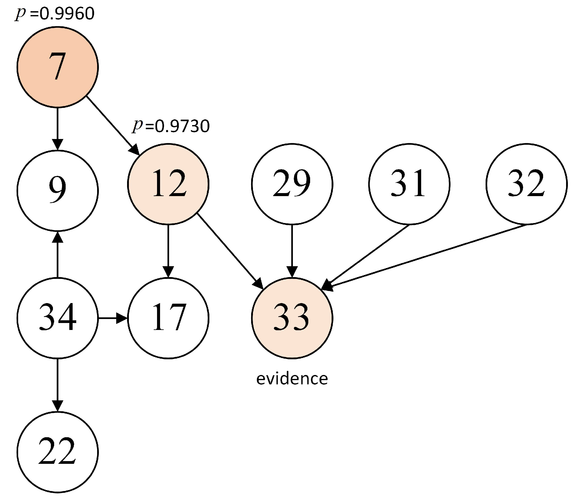
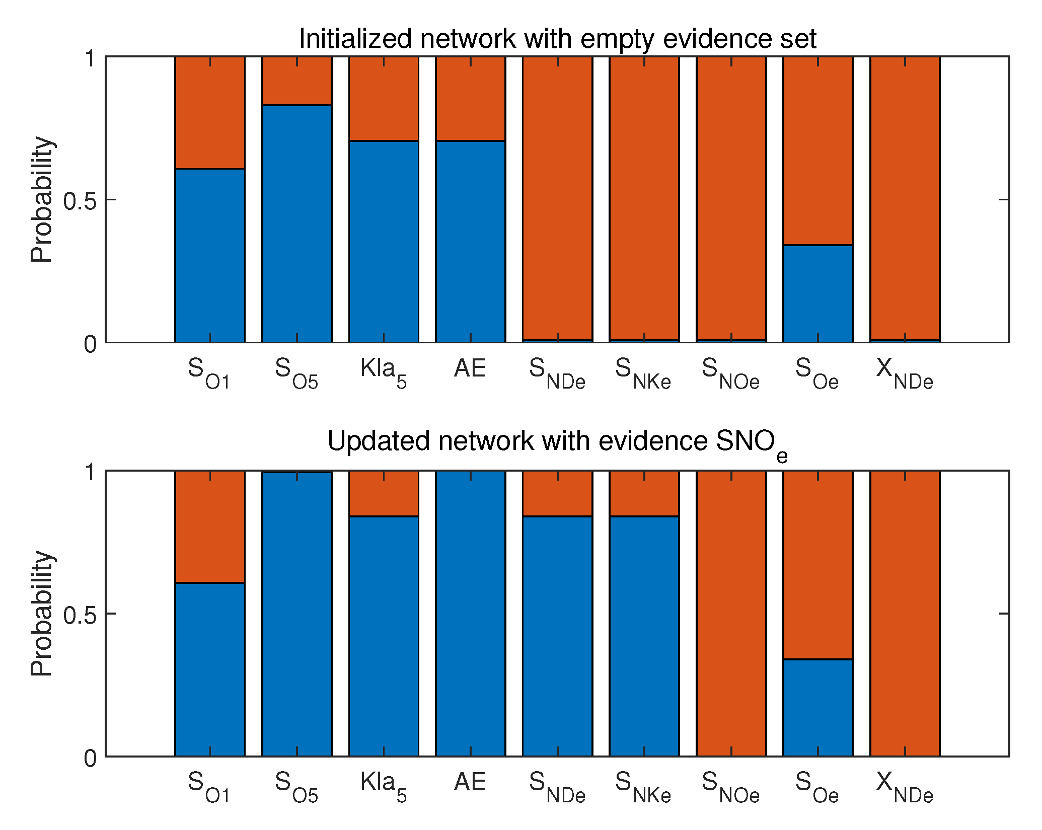
After constructing the causal network, we calculated the initial probability with MLE. Then, an evidence node was selected. According to knowledge on the process mechanism, effluent variables AE and PE were highly related to process operation quality. Therefore, one of the effluent variables with the highest contribution rate was considered to be the evidence node. Effluent variables were variables 29 and 31–36. Then, according to Figure 11, the evidence node of Dataset 1 was variable 27, and the evidence node of Dataset 2 was variable 33. We set the probability of evidence node to 1 and updated the network with a belief propagation algorithm. The results of Bayesian network inference are shown in Figure 17 and Figure 18, where the red part represents the probability of a nonoptimal state, and the blue part represents the probability of an optimal state. Detailed data are given in Table 3 and Table 4.
For Dataset 1, the evidence node was variable 26, which only had one parent node: variable 21. According to Table 3, after being updated, the probability of variable 21 changed from 0.83 to 0.9943. According to the result of PLS-GC, variable 21 had no parent node, but from the perspective of the mechanism, it had an indirect causal relationship with variable 1. This causal relationship is marked with a dashed line in Figure 14, but variable 1 showed no obvious change in probability update. Therefore, the root cause was variable 2, S Or 5 . The cause of the nonoptimal state was identified correctly.
For Dataset 2, results could be analyzed the same way. The evidence node was variable 33, which had four parent nodes: variables 12, 29, 31, 32. After being updated, only the probability of variable 12 greatly increased, to 0.9730. The parent node of variable 12 was variable 9, which increased to 0.9960. Therefore, the root cause was variable 7, S NOr 2 . The nonoptimal root cause of Dataset 2 was identified correctly. We compared our result with that of the traditional contribution-plots method. Figure 13 shows that the variables with the largest contribution rate were variables 21 and 33. Only the root cause of Dataset 1 was correctly identified, while variable 33 was not the root cause of Dataset 2. Such a comparison shows that the proposed method could identify the root cause.

5. Conclusions

In previous works, it was difficult to determine the causal relationship between variables due to the complex variable coupling relationships in industrial processes. In this work, a complete framework from operating performance assessment to nonoptimal cause identification was established. This scheme could handle strong coupling between process variables by using PLS in GC. We also employed BN to identify the root cause according to evidence nodes, which could also find the transmission path of the nonoptimal cause in the causal network. This root-cause identification method can help field operators in taking corresponding measures to improve current operating performance. As a case study, we tested its effect on BSM1. According to the results, the proposed method could correctly identify the root cause.
However, this method still has a few limitations to be improved. On the one hand, because we used methods to transform the causal structure into an acyclic graph, these treatments may render the nonoptimal transmission path incomplete. This problem can be improved by using suitable methods for cyclic problems, such as the dynamic causality diagram. On the other hand, the process of root-cause identification still needs knowledge on the process mechanism to assign an evidence node. It may be helpful to design an evaluation index to select evidence nodes. In the future, we aim to conduct more indepth studies on these aspects.

Author Contributions

Methodology, Y.W.; software, Y.W.; validation, Y.W.; resources, W.Z.; data curation, D.Y. and Y.W.; writing—original draft preparation, Y.W.; writing—review and editing, D.Y., X.P. and H.C.; supervision, W.Z. and H.C.; project administration, X.P. and W.Z.; funding acquisition, X.P. and W.Z. All authors have read and agreed to the published version of the manuscript.

Funding

This work is supported by the National Key Research & Development Program—Intergovernmental International Science and Technology Innovation Cooperation Project (2021YFE0112800), National Natural Science Foundation of China (Major Program: 61890930-3), National Natural Science Fund for Distinguished Young Scholars (61925305), National Natural Science Foundation of China (62173145) and Innovative development project of the industrial internet in 2020 (TC200802D).

Institutional Review Board Statement

Not applicable.

Informed Consent Statement

Not applicable.

Data Availability Statement

Data used in this paper were generated by BSM1, which can be found at http://iwa-mia.org/benchmarking/.

Conflicts of Interest

The authors declare no conflict of interest.

Abbreviations

PCAPrincipal component analysis
DAGDirected acyclic graph
PLSPartial least squares
GCGranger causality
PLS-GCPartial-least-squares-based Granger causality
BNBayesian network
CPTConditional probability table
CEIComprehensive economic indicatory
ERSEconomic subspace
EISEconomic-independent subspace
MIMutual information
CCACanonical correlation analysis
SFASlow feature analysis
ADF testAugmented Dickey–Fuller unit root test
MLEMaximum likelihood estimation
BSM1Benchmark Simulation Model 1
OCIOverall cost index

References

  1. Ye, L.; Liu, Y.; Fei, Z.; Liang, J. Online Probabilistic Assessment of Operating Performance Based on Safety and Optimality Indices for Multimode Industrial Processes. Ind. Eng. Chem. Res. 2009, 48, 10912–10923. [Google Scholar] [CrossRef]
  2. Liu, Y.; Chang, Y.; Wang, F. Online process operating performance assessment and nonoptimal cause identification for industrial processes. J. Process Control 2014, 24, 1548–1555. [Google Scholar] [CrossRef]
  3. Liu, Y.; Wang, F.; Chang, Y. Online Fuzzy Assessment of Operating Performance and Cause Identification of Nonoptimal Grades for Industrial Processes. Ind. Eng. Chem. Res. 2013, 52, 18022–18030. [Google Scholar] [CrossRef]
  4. Liu, Y.; Wang, F.; Chang, Y. Operating optimality assessment based on optimality related variations and nonoptimal cause identification for industrial processes. J. Process Control 2016, 39, 11–20. [Google Scholar] [CrossRef]
  5. Chu, F.; Dai, W.; Shen, J. Online complex nonlinear industrial process operating optimality assessment using modified robust total kernel partial M-regression. Chin. J. Chem. Eng. 2018, 26, 775–785. [Google Scholar] [CrossRef]
  6. Liu, Y.; Wang, F.; Gao, F. Hierarchical Multiblock T-PLS Based Operating Performance Assessment for Plant-Wide Processes. Ind. Eng. Chem. Res. 2018, 57, 14617–14627. [Google Scholar] [CrossRef]
  7. Chang, Y.; Zou, X.; Wang, F. Multi-mode plant-wide process operating performance assessment based on a novel two-level multi-block hybrid model. Chem. Eng. Res. Des. 2018, 136, 721–733. [Google Scholar] [CrossRef]
  8. Lu, Q.; Jiang, B.; Gopaluni, R.B.; Loewen, P.D.; Braatz, R.D. Locality preserving discriminative canonical variate analysis for fault diagnosis. Comput. Chem. Eng. 2018, 117, 309–319. [Google Scholar] [CrossRef]
  9. Venkatasubramanian, V.; Rengaswamy, R.; Yin, K.; Kavuri, S. A review of process fault detection and diagnosis: Part I: Quantitative model-based methods. Comput. Chem. Eng. 2003, 27, 293–311. [Google Scholar] [CrossRef]
  10. Zou, X.; Wang, F.; Chang, Y. Process operating performance optimality assessment and non-optimal cause identification under uncertainties. Chem. Eng. Res. Des. 2017, 120, 348–359. [Google Scholar] [CrossRef] [Green Version]
  11. Cheng, H.; Wu, J.; Liu, Y.; Huang, D. A novel fault identification and root-causality analysis of incipient faults with applications to wastewater treatment processes. Chemom. Intell. Lab. Syst. 2019, 188, 24–36. [Google Scholar] [CrossRef]
  12. Li, G.; Joe, S.; Tao, Y. Data-driven root cause diagnosis of faults in process industries. Chemom. Intell. Lab. Syst. 2019, 1859, 1–11. [Google Scholar] [CrossRef]
  13. Pearl, J. Causality; Cambridge University Press: Cambridge, UK, 2009. [Google Scholar]
  14. Granger, C.W.J. Investigating Causal Relations by Econometric Models and Cross-spectral Methods. Econometrica 1969, 37, 424–438. [Google Scholar] [CrossRef]
  15. Chen, H.S.; Yan, Z.; Zhang, X.; Liu, Y.; Yao, Y. Root cause diagnosis of process faults using conditional Granger causality analysis and Maximum Spanning Tree. IFAC-PapersOnLine 2018, 51, 381–386. [Google Scholar] [CrossRef]
  16. Kannan, R.; Tangirala, A.K. Correntropy-based partial directed coherence for testing multivariate Granger causality in nonlinear processes. Phys. Rev. E 2014, 89, 062144. [Google Scholar] [CrossRef]
  17. Chen, H.S.; Yan, Z.; Yuan, Y.; Huang, T.B.; Yi-Sern, W. Systematic Procedure for Granger-Causality-Based Root Cause Diagnosis of Chemical Process Faults. Ind. Eng. Chem. Res. 2018, 29, 9500–9512. [Google Scholar] [CrossRef]
  18. Lindner, B.; Auret, L.; Bauer, M. A Systematic Workflow for Oscillation Diagnosis Using Transfer Entropy. IEEE Trans. Control Syst. Technol. 2019, 28, 908–919. [Google Scholar] [CrossRef]
  19. Gharahbagheri, H.; Imtiaz, S.A.; Khan, F. Root cause diagnosis of process fault using KPCA and Bayesian network. Ind. Eng. Chem. Res. 2017, 56, 2054–2070. [Google Scholar] [CrossRef]
  20. Chen, G.; Ge, Z. Hierarchical Bayesian Network Modeling Framework for Large-Scale Process Monitoring and Decision Making. IEEE Trans. Control Syst. Technol. 2018, 28, 1–9. [Google Scholar] [CrossRef]
  21. Suresh, R.; Sivaram, A.; Venkatasubramanian, V. A hierarchical approach for causal modeling of process systems. Comput. Chem. Eng. 2019, 123, 170–183. [Google Scholar] [CrossRef]
  22. Gang, L.; Qin, S.J.; Zhou, D. Geometric properties of partial least squares for process monitoring. Automatica 2010, 46, 204–210. [Google Scholar]
  23. Stocchero, M.; De, N.M.; Scarpa, B. Geometric properties of partial least squares for process monitoring. Chemom. Intell. Lab. Syst. 2021, 216, 104374. [Google Scholar] [CrossRef]
  24. Pearl, J. Probabilistic Reasoning in Intelligent Systems: Networks of Plausible Inference. Artif. Intell. 1990, 48, 117–124. [Google Scholar]
  25. Cai, B.; Huang, L.; Xie, M. Bayesian networks in fault diagnosis. IEEE Trans. Ind. Inform. 2017, 13, 2227–2240. [Google Scholar] [CrossRef]
  26. Jin, S.; Liu, Y.; Lin, Z. A Bayesian network approach for fixture fault diagnosis in launch of the assembly process. Int. J. Prod. Res. 2012, 13, 6655–6666. [Google Scholar] [CrossRef]
  27. Zhao, Y.; Xiao, F.; Wang, S. An intelligent chiller fault detection and diagnosis methodology using Bayesian belief network. Energy Build. 2020, 57, 278–288. [Google Scholar] [CrossRef]
  28. Sun, W.; Paiva, A.R.; Xu, P.; Braatz, R.D. Fault detection and identification using Bayesian recurrent neural networks. Comput. Chem. Eng. 2020, 141, 106991. [Google Scholar] [CrossRef]
  29. Yu, J.; Rashid, M.M. A novel dynamic bayesian network-based networked process monitoring approach for fault detection, propagation identification, and root cause diagnosis. AIChE J. 2013, 59, 2348–2365. [Google Scholar] [CrossRef]
  30. Lo, C.H.; Wong, Y.K.; Rad, A.B. Bond graph based Bayesian network for fault diagnosis. Appl. Soft Comput. 2011, 11, 1208–1212. [Google Scholar] [CrossRef]
  31. Khanafer, R.M.; Solana, B.; Triola, J.; Barco, R.; Moltsen, L.; Altman, Z.; Lazaro, P. Automated diagnosis for UMTS networks using Bayesian network approach. IEEE Trans. Veh. Technol. 2008, 57, 2451–2461. [Google Scholar] [CrossRef]
  32. Wentian, L. Slow Feature Analysis: Mutual information functions versus correlation functions. J. Stat. Phys. 1990, 60, 823–837. [Google Scholar]
  33. Hotelling, H. Relations Between Two Sets of Variates. Biometrika 1935, 28, 321–377. [Google Scholar] [CrossRef]
  34. Wiskott, L.; Sejnowski, T.J. Slow Feature Analysis: Unsupervised Learning of Invariances. Neural Comput. 2002, 14, 715–770. [Google Scholar] [CrossRef]
  35. Ge, Z.; Zhang, M.; Song, Z. Nonlinear process monitoring based on linear subspace and Bayesian inference. J. Process Control 2010, 57, 676–688. [Google Scholar] [CrossRef]
  36. Dickey, D.A.; Fuller, W.A. Distribution of the Estimators for Autoregressive Time Series With a Unit Root. J. Am. Stat. Assoc. 1979, 74, 427–431. [Google Scholar]
  37. Wu, P.; Lou, S.; Zhang, X.; He, J.; Gao, J. Novel Quality-Relevant Process Monitoring based on Dynamic Locally Linear Embedding Concurrent Canonical Correlation Analysis. Ind. Eng. Chem. Res. 2020, 59, 21439–21457. [Google Scholar] [CrossRef]
  38. Liu, Y.; Pan, Y.; Huang, D. Development of a Novel Adaptive Soft-Sensor Using Variational Bayesian PLS with Accounting for Online Identification of Key Variables. Ind. Eng. Chem. Res. 2015, 54, 338–350. [Google Scholar] [CrossRef]
  39. Gernaey, K.V.; Jeppsson, U.; Vanrolleghem, P.A.; Copp, J.B. Benchmarking of Control Strategies for Wastewater Treatment Plants; IWA Publishing: London, UK, 2014. [Google Scholar]
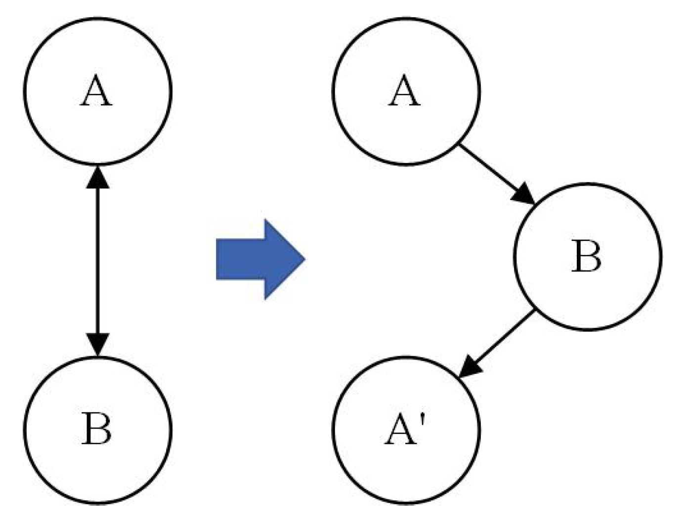
Figure 1. Illustrative diagram of duplicate dummy nodes.
Processes 10 00909 g001
Figure 2. Inference diagram of Bayesian network.
Processes 10 00909 g002
Figure 3. Schematic diagram of message passing in Bayesian network (a) variable elimination algorithm (b) belief propagation algorithm.
Processes 10 00909 g003
Figure 4. Schematic diagram of operating performance assessment.
Processes 10 00909 g004
Figure 5. Schematic diagram of root-cause identification.
Processes 10 00909 g005
Figure 6. Process of constructing network structure by PLS-GC.
Processes 10 00909 g006
Figure 7. Structural schematic diagram of BSM1 model.
Processes 10 00909 g007
Figure 8. Causal relationship between variables according to process mechanism.
Processes 10 00909 g008
Figure 9. Scatter diagram of offline performance grade division.
Processes 10 00909 g009
Figure 10. Classification result of test dataset.
Processes 10 00909 g010
Figure 11. Contribution plots of (a) Dataset 1 changing S O r 5 and (b) Dataset 2 changing S N O r 2 .
Processes 10 00909 g011
Figure 12. PLS-based granger causality results of (a) Dataset 1 changing S O r 5 and (b) Dataset 2 changing S N O r 2 .
Processes 10 00909 g012
Figure 13. Multivariate conditional granger causality results of (a) Dataset 1 changing S O r 5 and (b) dataset 2 changing S N O r 2 .
Processes 10 00909 g013
Figure 14. Causality network of Dataset 1.
Processes 10 00909 g014
Figure 15. Causality network of Dataset 2.
Processes 10 00909 g015
Figure 16. Causal network based on BSM1 mechanism (only relevant variables drawn).
Processes 10 00909 g016
Figure 17. Network update results of Dataset 1.
Processes 10 00909 g017
Figure 18. Network update results of Dataset 2.
Processes 10 00909 g018
Table 1. Selected process variables.
Variable NumberVariable Name
1, 6, 11, 16, 21Dissolved oxygen concentration of Tanks 1–5 S Or 1 S Or 5
2, 7, 12, 17, 22Nitrate and nitrite concentrations of Tanks 1–5 S NOr 1 S NOr 5
3, 8, 13, 18, 23Concentration of Tanks 1–5 S NHr 1 S NHr 5
4, 9, 14, 19, 24Soluble biodegradable organic nitrogen of Tanks 1–5 S NDr 1 S NDr 5
5, 10, 15, 20, 25Granular biodegradable organic nitrogen of Tanks 1–5 X NDr 1 X NDr 5
26Aeration intensity of fifth reaction tank Kla 5
27Aeration energy consumption, AE
28Pump energy consumption, PE
29Effluent speed Q e
30Internal reflux speed Q intrflow
31Soluble biodegradable organic nitrogen in effluent S NDe
32Effluent concentration of S NHe
33Effluent Kjeldahl nitrogen concentration S NKe
34Effluent concentration of nitrate and nitrite S NOe
35Effluent concentration of dissolved oxygen S Oe
36Effluent particulate biodegradable organic nitrogen X NDe
Table 2. Classification accuracy of test dataset.
GradesAccuracy of Proposed MethodAccuracy of Simple CCAAccuracy of Simple SFA
grade good0.98960.91700.9010
grade medium0.76010.67010.6963
grade poor0.87410.86360.8601
Table 3. Comparison of probability results before and after BN reasoning of Dataset 1.
VariablesInitial ProbabilityUpdated ProbabilityDifference
S Or 1 0.60730.60760.0003
S Or 5 0.83000.99430.1643
KLa 5 0.70450.83920.1347
AE 0.704510.2955
Q e 0.00810.83920.8311
S NDe 0.00810.83920.8311
S NOe 0.00810−0.0081
S Oe 0.34010.34010
X NDe 0.00810−0.0081
Table 4. Comparison of probability results before and after BN reasoning of Dataset 2.
VariablesInitial ProbabilityUpdated ProbabilityDifference
S NOr 2 0.81780.99660.1788
S NDr 2 0.81780.99660.1788
S NOr 3 0.75850.97300.2145
S NOr 4 0.54240.64340.1010
S NOr 5 0.81780.98970.1719
Q e 0.01270.0017−0.0110
S NDe 0.00420−0.0042
S NHe 0.13140.14330.0119
S NKe 0.796610.2034
S NOe 0.826310.1737
Publisher’s Note: MDPI stays neutral with regard to jurisdictional claims in published maps and institutional affiliations.