Numerical Simulations of a Postulated Methanol Pool Fire Scenario in a Ventilated Enclosure Using a Coupled FVM-FEM Approach

Abstract

Numerical investigations have been carried out for a postulated enclosure fire scenario instigated due to methanol pool ignition in a chemical cleaning facility. The pool fire under consideration is radiation-dominated and poses a risk to the nearby objects if appropriate safety requirements are not met. The objective of the current study was to numerically evaluate the postulated fire scenario and provide safety recommendations to prevent/minimize the hazard. To do this, the fire scenario was first modeled using the finite volume method (FVM) based solver to predict the fire characteristics and the resulting changes inside the enclosure. The FDS predicted temperatures were then used as input boundary conditions to conduct a three-dimensional heat transfer analysis using the finite element method (FEM). The coupled FVM–FEM simulation approach enabled detailed three-dimensional conjugate heat transfer analysis. The proposed FVM–FEM coupled approach to analyze the fire dynamics and heat transfer will be helpful to safety engineers in carrying out a more robust and reliable fire risk assessment.

1. Introduction

In the past few decades, an increase in chemical industry accidents has urged the demand to have strict regulations on the processing, storage, and transport of flammable materials [1]. Fires, explosions, gas clouds, and toxic gas dispersions are the four types of accidents in the chemical industry. Out of these, fire is considered one of the most frequently occurring types of accidents accounting for 41.5% of hazards [2]. Moreover, studies have even shown that pool fires occur more frequently than jet fires or flash fires [3]. Pool fires are buoyancy-dominated diffusion flames and occur when a flammable liquid kept inside an open vessel or confined in a specific area ignites accidentally [4]. There have been many incidents of pool fires in India, some of which have caused significant life and property losses. One such fire broke out at Indian Oil’s petroleum terminal at Jaipur in Rajasthan on 29 October 2009, when a tank containing 8000 kiloliters of oil was ignited [5]. The blaze continued to rage out of control for over a week, killing 12 people and injuring over 200 [6]. Many devastating pool fire accidents have occurred in chemical industries, which have compelled precautionary fire safety investigations for better building design plans and evacuation strategies [7,8].

Several researchers have been trying to predict pool fire behavior over the years due to the tumultuous, turbulent, and highly unpredictable flame structures [9,10,11]. Recently, a few researchers have also combined structural analysis with CFD using fluid–structure interaction algorithms [12]. Predicting pool fire characteristics using experimental techniques, developing numerical models based on the first principle, and validating them for different fire cases are the active areas of research [13,14,15]. Some of the most significant works that have been reported are that of Munoz et al. [16], Weckman and Strong [17], Chatris et al. [18], and Hamins et al. [19]. Researchers have experimentally studied pool fire characteristics of flammable materials ranging from hydrocarbons to alcohols in these studies [20]. Some of the noticeable works performed for validation of field models are those of Wen et al. [21], Chun et al. [22], Chung [23], and Vasanth et al. [24]. These researchers have assessed different CFD combustion, turbulence, and radiation models to validate and modify empirical models [25,26,27].

Fire modeling has become an essential part of fire safety research, as it is relatively less costly than experimental studies. Numerical simulations also can reproduce fire scenarios that cannot be recreated experimentally [5,28]. Fire Dynamics Simulator (FDS) is one of the most validated CFD packages designed specifically for modeling combustion, and hence it is used widely for research by practicing engineers and scientists [29].

Several simulation studies have been reported on enclosure fires in recent times [30,31,32]. Wen et al. [21] assessed the laminar flamelet approach (LFA) and the eddy dissipation concept (EDC) based LES solver FDS to simulate a methanol pool fire with a total heat release rate of 24.4 kW. The prediction of LFA and EDC combustion models was found to agree with each other and the experimental data of Weckman and Strong [17]. Yang et al. [33] simulated four different sets of ventilated enclosure fires to determine the sensitivity of the mixture models and the turbulence parameters on the fire characteristics. They found that the upper layer temperature predictions done using a two-step mixture model are highly sensitive to the size of the fire being simulated. They also reported that the turbulence parameters such as the Smagorinsky constant and turbulent Prandtl number do not strongly affect the total heat release rate and upper layer temperature predictions.

Vasanth et al. [24] evaluated various turbulence models to determine the most appropriate time-averaged model for simulating pool fires. They tested the standard k-ε model, realizable k-ε model, and the standard k-ω model for the combustion simulations. The validation studies that they carried out by comparing the flame shape, flame tilt, and temperature profile against experimental results showed that the standard k-ε model yields better results than the other two models tested. Vasanth et al. [34] investigated the burning rates of multiple pool fires by evaluating pool size and the separation distance between pools. They used the standard k-ε turbulence model and the eddy dissipation concept in commercial software ANSYS Fluent for simulating the combustion. They found that air entrainment rate is critical in determining the burning rates of multiple pool fires. The role of air entrainment can be understood by the results reported by Jain et al. [35]. Jain et al. [35] showed that enclosure fire temperature and velocity profiles are highly susceptible to ventilation. In addition, Vasanth et al. [34] also showed that the flame temperature, flame height, and burning rate of multiple pool fires are directly proportional to the diameter of the participating pools. Subsequently, they extended their pool fire research to fires resulting from different fuels [36].

Chen et al. [37] extended the EDC (initially developed for RANS models) to an LES-based FireFOAM solver. The HRR, radiative fraction, turbulent heat flux, SGS, total dissipation rate, kinetic energy, length scales, and time scales calculated by Chen et al. [37] were in fair agreement with the experimental data by Weckman and Strong [17].

In the present study, the FDS solver simulates methanol pool fires. The objectives of the current study are as follows: (i) validate the FDS solver against experiments for simulating a methanol pool fire (ii) use this validated model to carry out simulations of a postulated 2 m² enclosure based pool fire. (iii) Estimate the enclosure and flame temperatures considering all three modes of heat transfer. The limitations due to inherent assumptions in FDS are then addressed by using a new FDS (Finite Volume Method)—COMSOL (Finite Element Method) coupled approach. The combined observations from the FDS and COMSOL simulations have been used to conclude the current study.

2. Modeling and Simulation

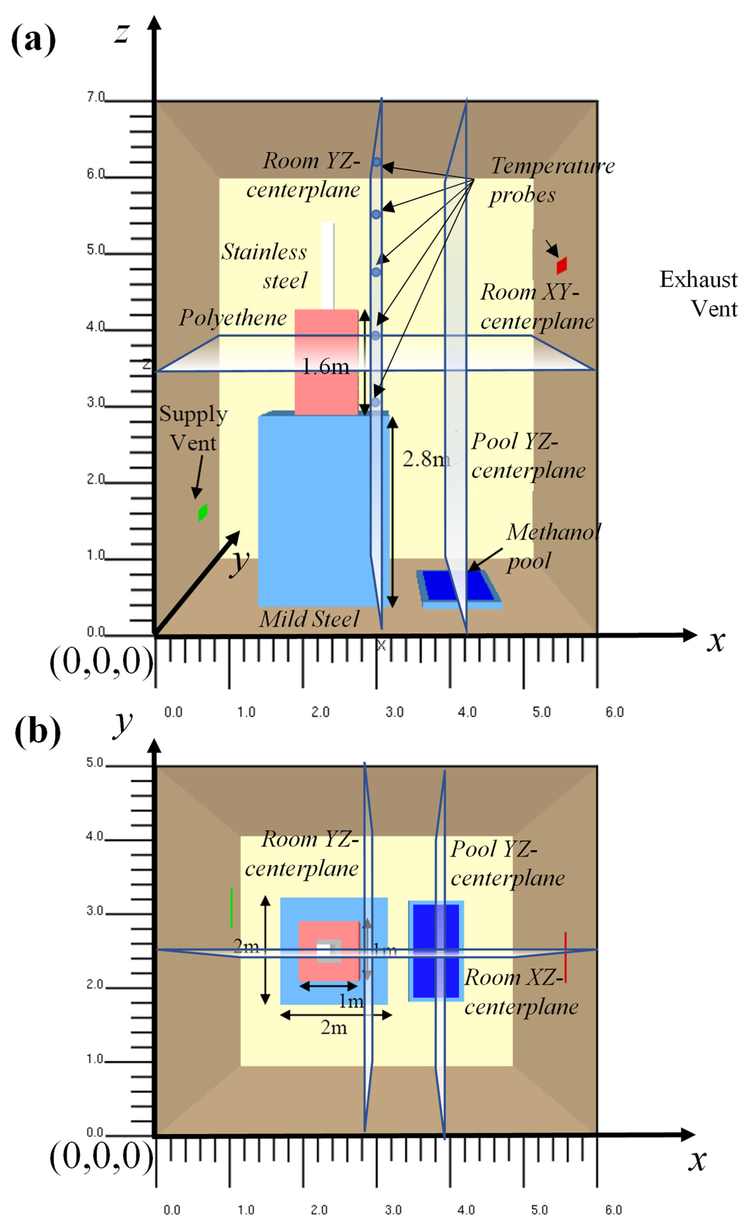
2.1. Problem Scenario

The scenario postulated involves leakage of methanol from a tank. The liquid methanol gets confined in a dike of area 2 m² inside an enclosure. The methanol pool is then postulated to ignite, resulting in a pool fire. A potential worst-case scenario of the postulated fire accident is to be simulated. The complete inventory of 200 L of methanol was considered to ignite. The enclosure is provided with a mechanical ventilation system. Sufficient oxygen is available for complete combustion of the methanol pool. The impact of the fire and incident thermal radiation on the cleaning system is to be assessed.

2.2. Model Description

The alcohol cleaning system is placed inside a concrete enclosure having dimensions of 5 m × 6 m × 7 m. A push and pull type ventilation is provided in the enclosure to maintain a ventilation rate of five air changes per hour. This was done using a supply and exhaust type ventilation where the inlet ventilation velocity was prescribed as 1.7 m/s, and the outlet ventilation rate was set to 2 m/s. The simplified diagram of the alcohol cleaning system is depicted in Figure 1.

The top view and the front view of the system, along with the illustration of the system’s main components, are shown in Figure 1.

The room shown in Figure 1 of the manuscript consists of a metallic-tube cleaning system that has stainless steel chamber (white block in Figure 1). During industrial operations, metallic tubes are placed inside this stainless steel chamber to be washed with methanol to remove any impurities that may have adhered to them during their manufacturing. For simulation purposes, a solid block of stainless-steel chamber was used. In reality, metallic tubes are placed inside the stainless-steel chamber. These metallic tubes have thermal properties similar to stainless steel, justifying the simplification of assuming the chamber to be made of solid stainless steel.

The stainless steel chamber is supported by mild-steel support (blue-block), while the above portion of the stainless steel chamber is shielded using polyethylene, (i.e., the pink block in Figure 1). A confined area with a pump and a tank is situated just a few inches away from the cleaning system. Methanol is stored in this tank, and pumped inside the stainless steel chamber to clean the metallic tubes.

2.3. Assessment Methodology

The pool fire of methanol is initially characterized to determine essential parameters such as burning rates, heat release rate, flame heights, centerline temperature, centerline velocities, and hot gas layer temperatures using various empirical correlations available in the literature. The incident thermal flux and heat transfer to the cleaning unit has been estimated. These empirical models have been developed based on experiments conducted under specific pressure, temperature, and humidity ranges for certain open or closed fire conditions. Many of these correlations do not consider factors such as the effect of changing ventilation rates/wind speeds on the flame heights and the fire spread [38,39]. Using such empirical correlations to estimate the transport phenomena and fire dynamics may result in deviations from the actual parameters. Thus, the fire was simulated in the CFD-based fire modeling software Fire Dynamics Simulator to verify it and get better heat transfer predictions. It is necessary to validate the FDS model against experiments to confirm its validity for methanol pool fires. This validation study was performed for a 31 cm diameter methanol pool fire that Weckman and Strong [13] have experimentally reported. A sensitivity analysis was carried out to determine the grid size capable of providing satisfactory predictions of the centerline temperature, centerline velocity, and hot gas layer temperature. The optimum fire diameter to grid size ratios obtained from the validation case was used for simulating the 2 m² methanol pool fire.

Though FDS has an excellent capability to predict the fire dynamics such as the flame temperatures, velocities, and radiative characteristics of the fire, it has certain limitations when considering the heat transport in solid objects. This is because FDS used a one-dimensional equation for modeling conduction heat transfer. Thus, the detailed study of heat transfer inside solid objects was simulated using COMSOL Multiphysics to overcome this limitation. The output temperature values obtained from the FDS were averaged and applied as input boundary conditions in COMSOL. A diagram explaining the sequence of flow for the assessment methodology is shown in Figure S1 of the Supplementary Information Section.

3. Governing Equations

Equations (1)–(3) provide the general mass, momentum, energy, and species balance in the Cartesian coordinate, which is used to represent the present system [40,41,42],

$$\frac{\partial \rho }{\partial t}+\nabla \cdot \left(\rho \mathrm{V}\right)=0$$

(1)

$$\frac{\partial \left(\rho V\right)}{\partial t}+\nabla \cdot \left(\rho u\mathrm{V}\right)=-\nabla p+\nabla \cdot {\tau }_{ij}+\rho f_x$$

(2)

$$\frac{\partial \left(\rho h\right)}{\partial t}+\nabla \cdot \left(\rho h\mathrm{V}\right)-\frac{\partial p}{\partial t}-V\cdot \nabla p={\dot{q}}^{″}+\nabla \cdot k\nabla T+\nabla \cdot h_l{\left(\rho D\right)}_l{Y}_l$$

(3)

$$\frac{\partial }{\partial t}\left(\rho Y_l\right)+\nabla \cdot \rho Y_{l}V=\nabla \cdot {\left(\rho D\right)}_l\nabla Y_l+l{\dot{W}}_l^{‴}$$

(4)

The large eddy simulation (LES) model was used for FDS simulations in the present study. The details of the LES model used have been specified below.

For solving the energy equation in FDS, the constant temperature boundary condition is used where a constant temperature is prescribed at the solid surface. The surface material is assumed to be thermally thick material, and the one-dimensional heat conduction equation is applied in the direction n normal to the solid surface (Equations (4) and (5)).

$${\rho }_s{c}_s\frac{\partial T_s}{\partial t}=k_s\frac{{\partial }^2{T}_s}{\partial n^2}$$

(5)

As opposed to the above boundary condition, the energy equation in COMSOL considers the three-dimensional heat conduction equation as specified below (Equation (6)).

$${\rho }_s{c}_s\frac{\partial T_s}{\partial t}=\frac{\partial }{\partial x}\left(k_s\frac{\partial T_s}{\partial x}\right)+\frac{\partial }{\partial x}\left(k_s\frac{\partial T_s}{\partial x}\right)+\frac{\partial }{\partial x}\left(k_s\frac{\partial T_s}{\partial x}\right)+\dot{q}$$

(6)

3.1. Large Eddy Simulation (LES)

The basic concept of this model is applying a filter of specific cut-off lengths to distinguish the large-scale eddies from the small-scale eddies. The large-scale eddies are resolved directly, while the smaller eddies are modeled. The fluctuations and randomness of flows are better predicted using LES models rather than RANS. Though LES is more computationally expensive than RANS, it can predict the behavior of complex flows more efficiently and accurately than the RANS models [43]. Fires are highly turbulent, and LES is the most suitable turbulence model for adequately resolving the essential time and length scales for such turbulent flows, that too at a computational cost lesser than that required for DNS [44,45].

The spatial filtering operation in LES for any transported field is defined by using a filter function (Smagorinsky [46]). A cut-off width Δ is used to filter out the eddies resulting in a space filtered form of variable, represented by an overbar. The filtering operation implies that eddies of size larger than Δ are large eddies, i.e., these eddies are resolved directly, while eddies smaller than Δ are small eddies that must be modeled [47]. The selection of cut-off width Δ is user-dependent.

Generally, for structured meshes, the value of Δ is found using the Equation (7)

$$\Delta =\sqrt[3]{{\Delta }_x{\Delta }_y{\Delta }_z}$$

(7)

Here, Δ_x, Δ_y, and Δ_z are the length, width, and height, respectively, of a typical hexahedral element. A filtered form of the momentum equation is obtained by applying the filtering operation to the generalized momentum equation, as shown below in the Equation (8).

$$\frac{\partial \left(\rho \overline{\overline{u}}\right)}{\partial t}+\nabla .\left(\rho \overline{\overline{uv}}\right)=-\nabla \overline{\overline{p}}+\nabla .\overline{\overline{{\tau }_{ij}}}$$

(8)

Here, $\overline{\overline{{\tau }_{ij}}}=\mu \left(\frac{\partial \overline{\overline{u}}}{\partial y}+\frac{\partial \overline{\overline{v}}}{\partial x}\right)$.

The Equation (9) shows that the convective terms of the resolved velocity field and sub-grid stress (SGS) tensors are introduced.

$${\tau }_{ij}^s=-\rho \left(\overline{\overline{uv}}-\overline{\overline{u}}\overline{\overline{v}}\right)$$

(9)

The above SGS stress tensor represents large-scale momentum flux caused by small or unresolved scales, and it must be modeled to ensure closure. After including the SGS term, the filtered momentum equation can be expressed as shown in the Equation (10)

$$\frac{\partial \left(\rho \overline{\overline{u}}\right)}{\partial t}+\nabla .\left(\rho \overline{\overline{u}}\overline{\overline{v}}\right)=-\nabla \overline{\overline{p}}+\nabla .\left(\overline{\overline{{\tau }_{ij}}}+{\tau }_{ij}^s\right)$$

(10)

${\tau }_{ij}^s$ is further obtained using SGS models in the Equation (11).

$${\tau }_{ij}^s=-2{\mu }_e{\overline{\overline{S}}}_{ij}+\frac{{\tau }_{kk}^s{\delta }_{ij}}{3}$$

(11)

where, ${\mu }_e$ is the SGS eddy viscosity. ${\overline{S}}_{ij}$ is given by the Equation (12)

$${\overline{\overline{S}}}_{ij}=\frac{1}{2}\left(\frac{\partial \overline{\overline{u}}}{\partial y}+\frac{\partial \overline{\overline{v}}}{\partial x}\right)$$

(12)

The Deardoff [48] model is the recommended SGS model for simulating pool fires [21,33,49] and was thus used to carry out simulations in the present case. The SGS eddy viscosity term as per the Deardoff [48] model is given as follows (Equations (13) and (14)):

$${\mu }_e=\rho C_v\Delta \sqrt{k_{sgs}}$$

(13)

where,

$$k_{sgs}=\frac{1}{2}{\left(\overline{u}-\widehat{u}\right)}^2+{\left(\overline{v}-\widehat{v}\right)}^2+{\left(\overline{w}-\widehat{w}\right)}^2$$

(14)

Here $\overline{u}$ is the average value of u at the grid cell center and $\widehat{u}$ is the weighted average value of u over the adjacent cells. Similarly, $\overline{v},\widehat{v},\overline{w}$ and $\widehat{w}$ are the average values of v and w along the cell centers and over the neighboring cells, respectively. C_v is a constant and takes the value of 0.1 [48].

The constitutive model equations specified above are discretized using a second-order predictor correction scheme. The time step chosen for both the fire modeling and conduction modeling satisfies the Courant–Friedrichs–Lewy condition. A residual of 10⁻⁴ has been specified for all the governing equations. The time step size selected converged as per the prescribed residual values within 50 iterations per time step.

3.2. Fire Modeling

FDS is a large eddy simulation (LES) turbulence model-based computational fluid dynamics solver for low Mach number-driven flows. Unlike RANS models, LES models are inherently time-dependent [42,43]. The LES model is fundamentally based on applying a filter to screen out the large-scale eddies and small-scale eddies wherein the former would be resolved. The latter would be modeled using favorable sub-grid-scale models. This filtration is based on the large-scale eddies being the most effective transporters of conserved quantities than the small-scale ones. So, the larger eddies get fully resolved, yielding more accurate flow predictions than RANS. The basic equation for the LES turbulence model is explained in detail in the previous sections. Some sub-grid-scale (SGS) models have been proposed, and different models are efficient in various flow applications. Thus, the selection of SGS models largely depends on their efficiency for that specific field of application. Similar is the case for the various constants used in the SGS equations and the values of turbulent Prandtl number and turbulent Schmidt number (which by default are set to 0.5) (McGrattan et al. [29]). The Deardoff [48] SGS model in FDS (McGrattan et al. [29]) has been shown to capture the dynamics of pool-fire flames accurately in several studies [50,51,52]. Thus, the Deardoff [48] SGS model was carried out in the present investigation.

The most crucial part of the simulation of any given fire scenario is modeling the flame thickness, which may be as small as one millimeter. The flame is appropriately captured by the closures of the mean chemical mass production rate of species’ α’ per unit volume ${\dot{m}}_{\alpha }^{‴}$ (McGrattan et al. [29]). A partially stirred batch reactor model is used in FDS, which can efficiently solve non-premixed combustion. The Equation (15) for heat release rate per unit volume (${\dot{q}}_{\alpha }^{‴}$) in this combustion model is given as follows:

$${\dot{q}}_{\alpha }^{‴}=-{\displaystyle \sum _{\alpha }{\dot{m}}_{\alpha }^{‴}}\Delta h_{f,\alpha }$$

(15)

where, ${\dot{m}}_{\alpha }^{‴}$ is the mass production rate of the species α per unit volume, $\Delta h_{f,\alpha }$ is the heat of formation of the burning material. FDS uses a lumped species approach, which reduces computational load by combining species into groups, as shown below.

Fuel + Air → Products

Reactants → Fuel, oxygen, N₂

Products → CO₂, H₂O, N₂

4. Validation of FDS

The methanol pool fire modeling has been done by comparing the flame height and temperature obtained from simulations to those reported by Weckman and Strong [17]. The physical properties of the simulation setup are the same as those reported by Weckman and Strong [17]. The techniques implied for building the geometry, meshing the domain, and applying the respective boundary conditions are explained below.

4.1. Geometry and Meshing

Weckman and Strong [17] performed experiments on a 31 cm circular methanol pool fire to investigate the fire’s turbulence, centerline temperature, velocity, and hot gas layer temperatures. A pool fire of the same dimension has been set up in FDS, as shown in Figure 2. This study created a circular pan for the fire using the newly developed ‘Circular Vents’ technique described in detail in McGrattan et al. [29]. The Cartesian coordinate system is used to generate a domain of dimensions 1.6 m (width) × 1.6 m (depth) × 3.2 m (height). The ground was solid while all other boundaries were set as open. An open boundary condition assumes that ambient conditions exist for the surface to which it is prescribed. The open boundary condition can only be prescribed at an exterior boundary of the computational domain. The open boundary condition uses a constant pressure assumption (in the present case, it is the ambient pressure). The methanol feed rate is 1.35 cm³/s with a mass loss rate per unit area boundary condition. Three different mesh sizes, i.e., coarse, medium, and fine, were tested for sensitivity analysis. The grid sizing used in the simulation is based on the sensitivity analysis listed in

Table 1. Grid sizing chose for sensitivity analysis of the validation case.

Grid Size	Criterion of Classification	W × D × H	Size of Each Cell	Total No. of Cells
Coarse	$D^{*}/dx=4.36$	32 × 32 × 48	0.05 m	49,152
Medium	$D^{*}/dx=6.54$	48 × 48 × 96	0.033 m	22,184
Fine	$D^{*}/dx=10$	75 × 75 × 150	0.0218 m	843,750

.

The cell size dx and the characteristic fire diameter D* are related. A smaller characteristic fire diameter must be accompanied by a more refined cell size so that a greater amount of turbulent energy is solved on grid points.

The characteristic fire diameter, D*, is given by the Equation (16) as per the definition of McGrattan et al. [29]

$$D^{*}={\left(\frac{\dot{Q}}{{\rho }_{\infty }{c}_{\infty }{T}_{\infty }\sqrt{g}}\right)}^{\raisebox{1ex}{$2$}\!\left/ \!\raisebox{-1ex}{$5$}\right.}$$

(16)

where, ${\rho }_{\infty }$, $c_{\infty }$ and $T_{\infty }$ are density, specific heat, and temperature at ambient conditions. In this study, the $\dot{Q}$ value has been determined to be 24.6 kW. From the Equation (16), it was found that the characteristic fire diameter D* = 0.218 m.

The optimum mesh size obtained from the validation case was used as the basis for meshing the geometry of the postulated scenario. Results from the validation case showed that better predictions were obtained for $D^{*}/dx=10$. Thus, for the postulated scenario too, the $D^{*}/dx$ was maintained as 10. By using this ratio, the entire domain was around five million cells, where the finest cell sizes were maintained near the solid walls and liquid pool (ranging from 0.003 m to 0.0075 m), while the maximum cell sizes went up to 0.01 m.

4.2. Boundary Conditions

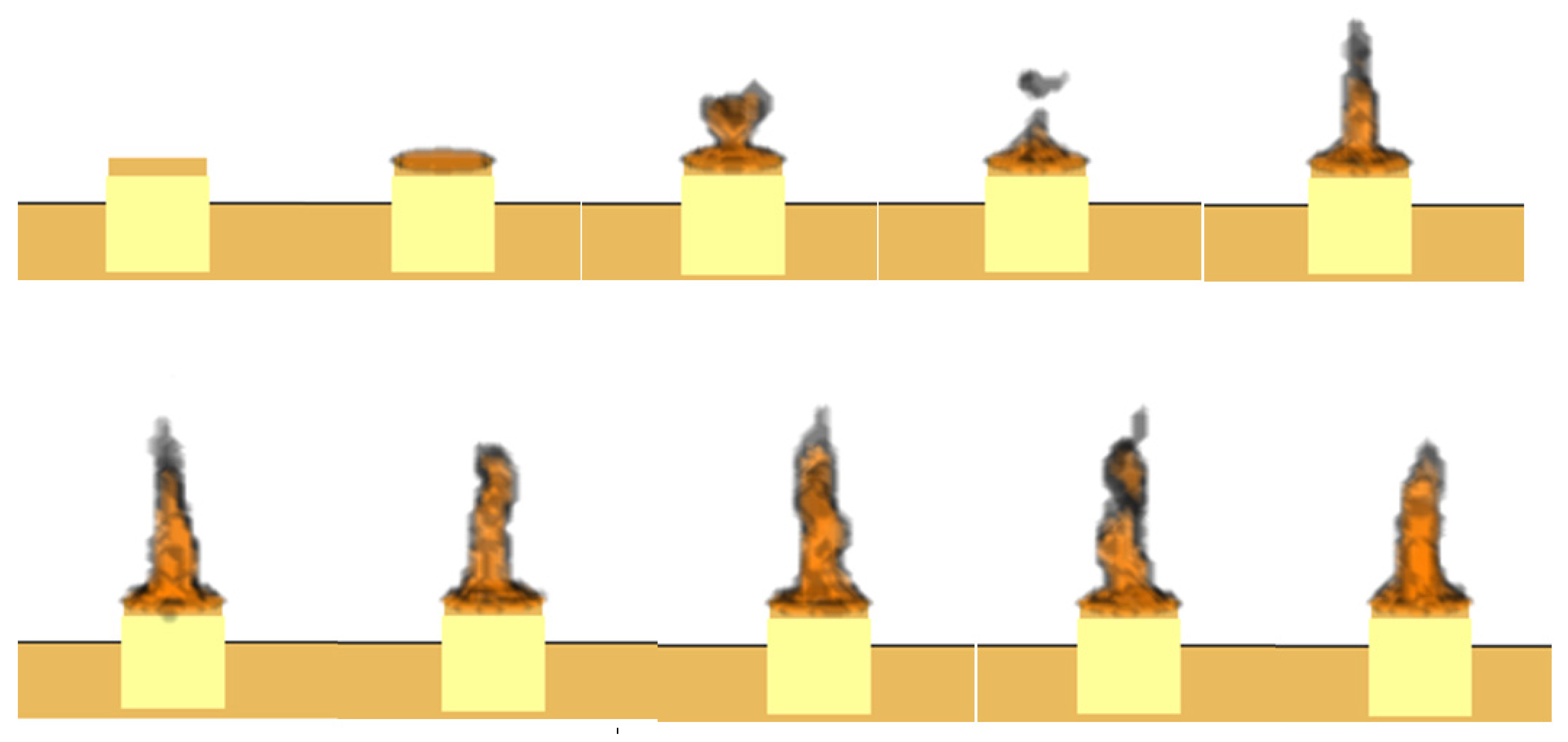
The radiative fraction of 0.15 and the volumetric flow rate of 1.35 cm³/s were prescribed to define the methanol fuel [9]. The other physicochemical properties of methanol have been stated in the Supporting Information Section. This flow rate was provided as an input boundary condition in the form of mass loss rate per unit area (0.015 kg/m² s) to model the combustion as per the experiments of Weckman and Strong [17].

Since both these values have been input as boundary conditions, FDS can calculate the heat flux, and thereby, the combustion phenomenon will occur for all the length and time scales where the mixing of air and fuel occurs.

Additionally, the temperature was set as follows: at t = 0, T = 20 °C. So, the initial temperature for the entire domain is 20 °C. As the simulation begins, the combustion will occur, and the temperature will increase temporally and spatially. The increasing temperature depends on the heat flux produced by combustion, which takes place. The simulations were run once the geometry, meshing, and boundary conditions were provided for the validation case.

4.3. Fire Ignition

The validation case of methanol pool fire was run for 20 s as it was found to attain a steady-state under this time duration. The simulation’s initial condition was that at t = 0, T = 20 °C, there was no fire initially. As the simulation begins and time proceeds, the fire ignites and further develops towards attaining a steady state. Figure 3 below shows the fire’s time frames every two seconds, starting from t = 0 s to t = 18 s. An initial pulsating nature of the flame is witnessed in Figure 3, which is in line with the experimental results of Weckamn and Strong [17]. Thus, the prediction for the development of the fire is in good agreement with the experimental results.

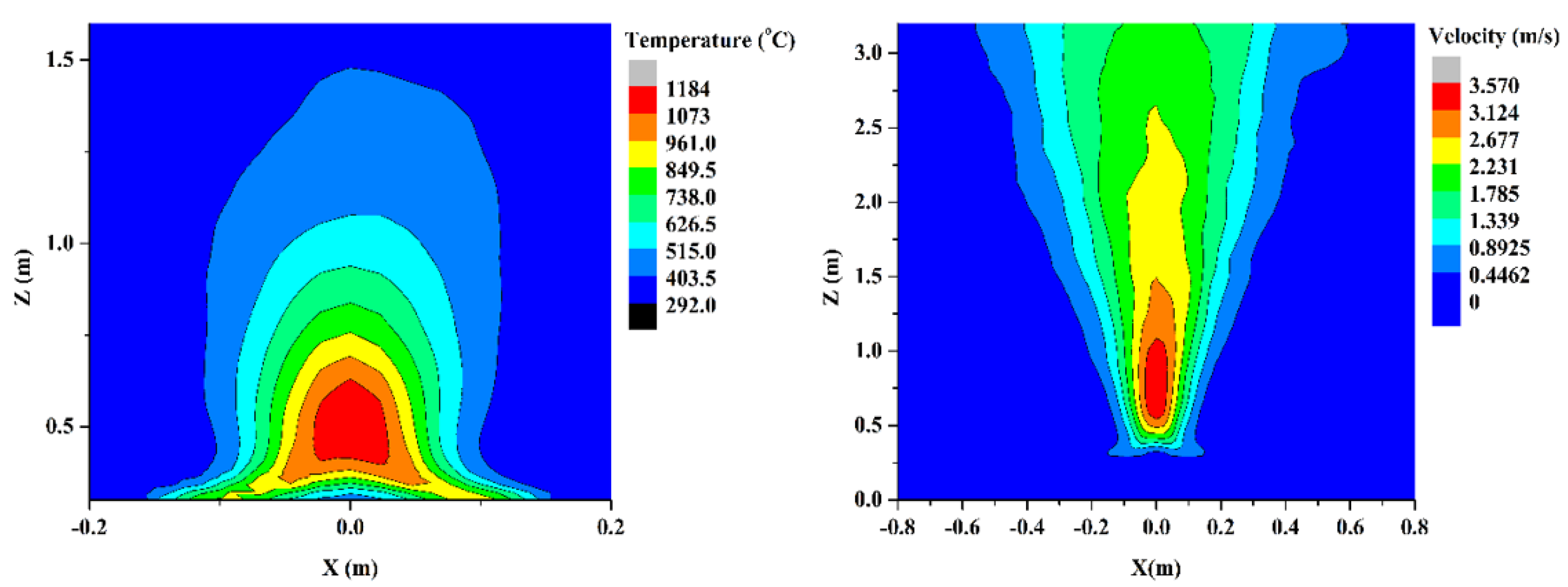
4.4. Velocity and Temperature Profiles

For validation purposes, a sensitivity analysis is done using the mesh sizes specified in Table 1. The centerline temperatures and velocities are measured at 6, 12, 20, and 30 cm from the pan’s methanol fuel. In addition, the hot gas layer temperatures are measured and compared with the experimental values. Figure 4 gives a clear picture of the average centerline temperature and velocity obtained for the validation case. The temperatures near the fuel surface have the highest values, decreasing as the height increases. The temperatures are highest near the fuel surface as the mixing of the fuel and oxygen is maximum near the fuel surface. Due to buoyancy effects, the vaporized fuel concentration further diffuses at certain heights above the fuel surface. It gradually mixes with the fresh air, decreasing the temperature above the liquid pool at higher altitudes. On the other hand, as diffusion is greater within the flame region, the velocity in this region is the highest while decreasing at increasing heights above the flame.

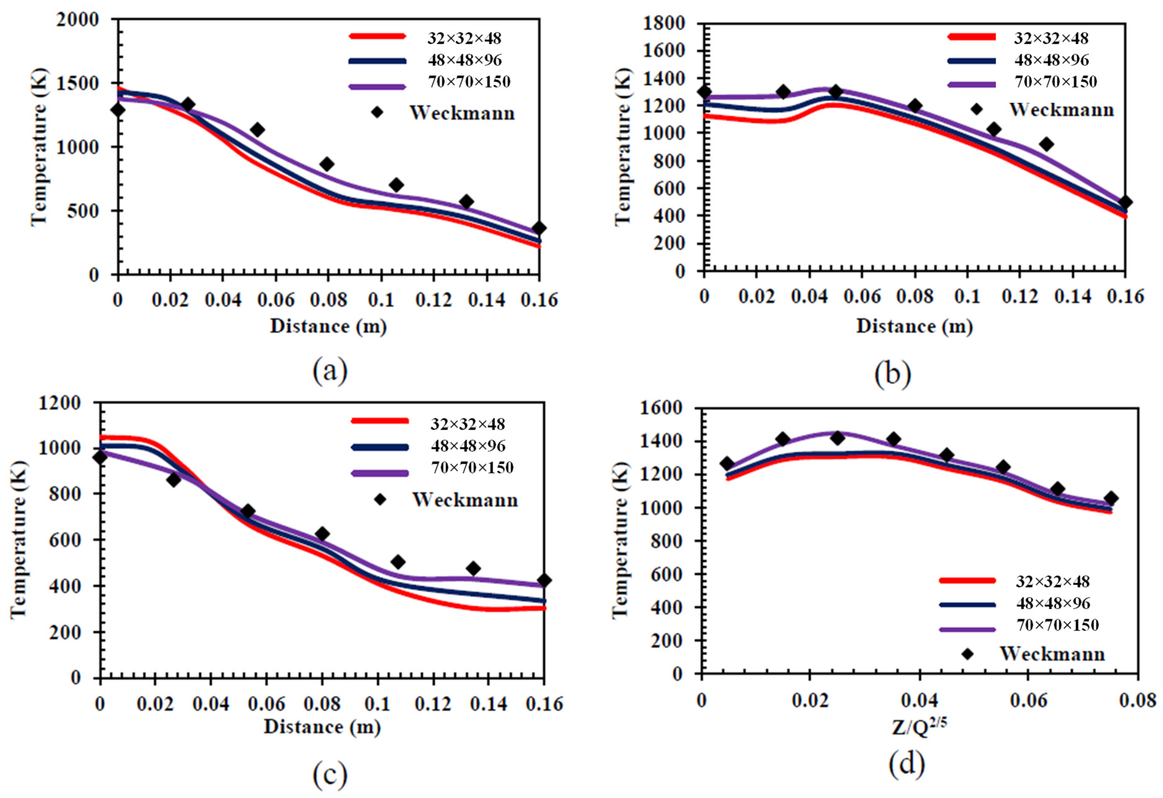
4.5. Sensitivity Analysis

It was found that the values of the hot gas layer, centerline temperature, and centerline velocities were underpredicted for the coarsest mesh size. This happened because the coarse mesh cannot capture the turbulence produced for smaller lengths and time scales, thus causing poor predictions. The temperature predictions obtained for heights 6, 12, and 20 cm above the fuel layer are shown in Figure 1a–c, respectively. It was found that maximum temperature values are obtained closest to the fuel surface, i.e., at 6cm above the fuel surface. At this height, the maximum temperature values were as high as around 1400 K at the centerline and decreased radially towards the vessel wall. A similar trend with a somewhat lower maximum temperature value is obtained for heights 12 cm and 20 cm.

The analysis for the different mesh sizes shown in Figure 5 illustrates that the finest size mesh gives the most accurate temperature predictions. The maximum value of flame temperature predicted by FDS was at the height of 6 cm above the fuel surface along the centerline. This agrees with the maximum temperature at a similar height reported by Weckman and Strong [17]. This variation of values along the radial distances is minimal and thus can be neglected. The variation occurs since many temperature fluctuations occur in the region close to the fuel surface. Therefore, slight discrepancies in numerical predictions are bound to happen in this range. The temperatures at a further radial distance for all the three mesh sizes decrease with radial distances, with the lowest temperatures reported at maximum distances away from the centerline.

Though the trend followed by all three mesh sizes is similar to that reported by experimental results, it was found that the values are way less than the experimental results for the coarse-sized mesh. These values are slightly higher for the medium-sized mesh, but the best-predicted values are obtained only for the fine-sized mesh. Similar is the case for temperatures obtained at 12 cm and 20 cm above the fuel surface, i.e., the maximum temperature was obtained at the centerline with decreasing temperatures along with the radial distances away from the centerline. Additionally, the best results in these two cases were found when the fine-sized mesh was used. Figure 1b shows the hot gas layer temperature at different heights. For convenience, the hot gas layer is plotted against Z/Q^2/5 instead of Z alone. It is observed that the maximum temperature ranges occur at ratios of around 0.02 and 0.03; this is because, as fire starts and hot smoke emerges from this fire, the hot gases rise to certain heights before they start settling down. Thus, maximum temperatures are obtained for these ranges while the temperature for a ratio below 0.02 is lesser. In addition, as the smoke moves upwards, it mixes with the colder air above, and thus its temperature decreases. Therefore, for ratios greater than 0.03, the temperature further decreases.

After temperature, the centerline velocities were compared against the experimental predicted velocities of Weckman and Strong [17], which were found to be in good agreement with each other. The figures and corresponding text for the centreline velocities have been shown in the Supporting Information Section. The velocities at distances closer to the centerline were found to have a greater value than the center.

5. Results and Discussion

5.1. Results for the Postulated Scenario: Simulation I

Two simulations were set up in FDS for the postulated scenario. Simulation I, where no mild steel shield layer was applied over the polyethylene shield, and simulation II, where a mild steel layer covered the polyethylene shield from all four sides. The heat release rate, flame heights, incident heat flux, hot gas layer temperatures, and the centerline temperatures of the fire were the same for both these cases, which have been reported before the detailed explanation of case-specific results.

Initially, the room was at 25 °C, but as the ignition of the methanol pool took place and the hot gases from the fires started to rise due to buoyancy, the temperatures began to rise. The hot gases rise from the fire, hit the ceiling, and then downward. At the same time, fresh air enters the room from the supply vent, and the hot gases generated move out from the exhaust vent. It is evident from the plot in Figure 6 that the maximum temperature occurs at the height of 7 m, followed by the temperature at subsequent lower heights. The highest temperature occurs at the ceiling, where the hot gases accumulate before they gradually settle down. Thus, the highest hot gas layer temperature values are at 7 m, followed by 6 m, 5 m, 4 m, and 3 m, respectively. A gradual increase in temperature is noticed up to 500 s as the gases are still rising and settling down. However, after 500 s, the entire room is filled with gas, and the maximum temperature values have already been reached. As a result, a minimal increase in temperature occurs after 500 s at all heights.

Temperatures were extracted at five different locations along the centerline of the fire at a distance of 0.1 m, 0.5 m, 1 m, 1.5 m, and 2 m along the z-direction. The temperatures predicted from the simulations are shown in Figure 7. As observed in the plot, the highest temperatures are obtained at the location closest to the fuel surface, i.e., at 0.1 m, while the temperatures predicted at subsequent heights decrease. This can be explained by the same phenomenon of maximum mixing near the fuel surface earlier explained for the centerline temperatures obtained for the validation case. The temperatures seem to rise for 500 s, after which they attain a steady state. For a better understanding of the centerline temperature, a contour plot for the mean value of the centerline temperature is obtained and shown in Figure 8 below.

As seen in Figure 8, the temperature near the fuel layer is the highest, and the temperature decreases along the z-direction. This happens as the hot flames and gases diffuse to higher layers; they mix with the fresh air, resulting in decreased temperatures than observed at lower levels. The temperature near the ground surface adjacent to the pool area is the lowest as the hot gases descend there only after the hot gases fill the entire upper part of the room. Thus, when the hot gases descend, the temperature goes down. In addition, as the plot in Figure 8 represents the mean centerline temperatures, the maximum values for temperature are lower than the local centerline temperatures shown in Figure 7.

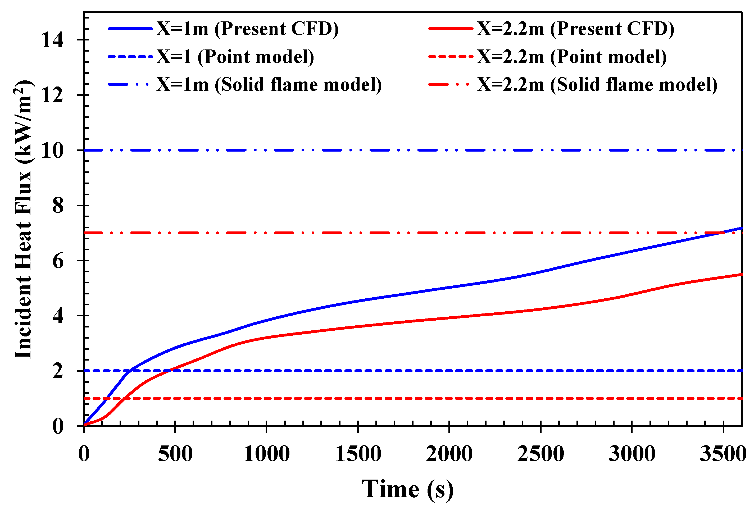
5.1.1. Incident Heat Flux

The incident heat flux predicted by FDS has been reported below in Figure 9. Incident heat flux in FDS measures convective and the inward radiative heat flux on an object located at a certain distance from the fire.

The shield facing the fire is exposed to the highest heat intensity and must be examined. This face is at a distance of one meter from the fire. It is found that the incident heat flux goes on increasing with time. After around one hour, the incident heat flux reaches a value of about 7 kW/m². This value is within the acceptable range of the steady-state incident heat flux values obtained by the point source model and the solid flame model, as shown in Figure 9.

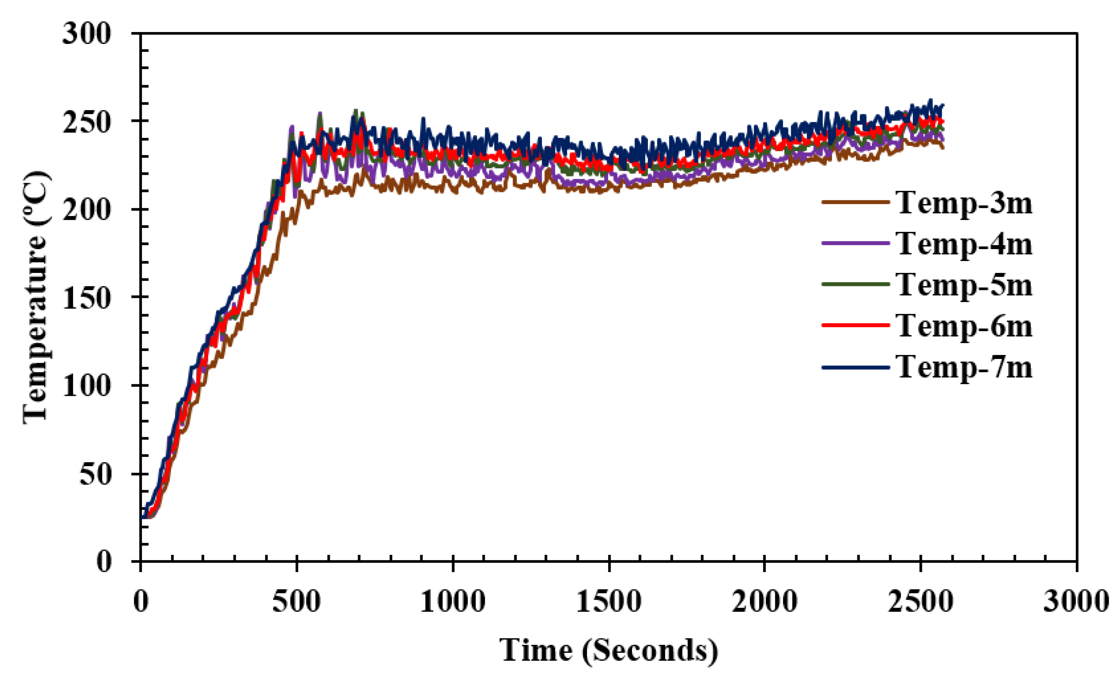
5.1.2. Enclosure Temperature

For better understanding, the sides of the shield in the cleaning system have been labeled and shown in Figure S6 of the Supporting Information File. The results for temporally evolving temperatures at all these sides are then reported.

It is noticeable that the temperature on the fire-facing side of the polyethylene shield did not rise to susceptible risks, up to 320 s. Thus, the temperature profiles after 320 s are only included here. Figure 10 shows the temperature profile for the cleaning system at 320 s. It is observed that the temperatures on the outer layer of the polyethylene shield have shot up to around 65 °C. The polyethylene shield can withstand a temperature of 65 °C, though it is an early warning that if the temperature continues to rise, it will soon reach its melting point, thus damaging the entire shield. Further increase in temperature was noted at 400 s.

Figure 10a shows that the maximum temperature was reached for the fire-facing side, i.e., side A, which was around 95 °C. The temperatures for the two adjacent sides and the backside, i.e., side B, side D, and side C, are shown in Figure 10b–d, which are found to be around 50 °C. The temperature profile for the fire-facing side also shows that the temperature on the right side is higher than that on the left side. This occurred due to the fresh air supply from the supply vent on the left side, keeping the temperature there somewhat lesser than the temperatures on the right. Additionally, higher temperatures at the top and lower at the bottom were observed because the upper part of the shield is directly incident to the flame while the lower part gets blocked by the stainless stand. Further, the hot gases descending from the ceiling also have higher temperatures at greater heights. The heat incident from the gases at higher elevation causes the temperature for the upper part to be higher than that of the lower part. Further, it was found that at 500 s, the temperature goes as high as 115 °C, which the polyethylene shield cannot withstand as this is the range at which polyethylene starts melting.

A mild steel shield was wrapped around the polyethylene to prevent it from melting. The thickness of the mild steel layer was determined as per a sensitivity analysis reported in Section S9 of the Supporting Information File. The simulations carried out for the system with a mild steel layer have been reported in the next section.

5.2. Results for the Postulated Scenario: Simulation II

In simulation II, a layer of mild steel sheet 200 mm in thickness was shielded on all four sides around the polyethylene. Mild steel is not expensive and can be used safely in chemical industries. The terminology for this change of a mild steel layer over the polyethylene shield has been shown in Figure S7 of the Supporting Information File.

5.2.1. Enclosure Temperature

Figure 11 illustrates the enclosure temperature and the temperature on other solid surfaces inside the enclosure. The contour plot has been plotted 500 s after the ignition of the methanol pool. As shown in Figure 11a,b, all the solid surfaces exhibit temperatures of 25 °C to 50 °C. It is only the temperature neat the exhaust vent and the methanol pool container which show temperatures higher than 50 °C. In contrast to this, from simulation I, the polyethylene temperature goes to as high as 100 °C within 500 s of combustion if the mild steel shield is not provided.

5.2.2. Velocity Profile

The velocity distribution contours have been plotted over the XZ center plane of the enclosure to visualize the inflow and outflow of fresh air and understand the flow patterns of the continuously evolving pool fire. Figure 12 shows that fresh air is coming from the supply vent and the hot gases coming out from the fire are escaping through the exhaust vent. The velocity distribution near the plume of the fire showed an average value of 3.8 m/s. The velocities are particularly more intense from the base of the methanol pool up to the flame height. The velocity values reduce gradually from the flame region to the top region of the enclosure. The gradual reduction in temperature occurs because the fresh air coming inside the enclosure from the supply vent and gases rising from the fire due to buoyancy (to be pushed out from the exhaust vent) get mixed, causing velocity magnitudes to go down.

5.2.3. Oxygen Availability

Figure 13a shows the oxygen concentration inside the enclosure 80 s after the ignition of the methanol pool. The left side of the enclosure is close to the supply vent and far from the location of the methanol pool fire. Thus, the left side of the enclosure still has a higher oxygen concentration (~0.20 mol/mol) after 80 s. The right side of the room is where the pool fire is burning, and thus it can be seen that there are several patches of oxygen concentration as low as 0.1 mol/mol in this region. The flame region can be seen to have the lowest oxygen concentrations. These range from values as low as 0.04 mol/mol to 0.1 mol/mol. The fire utilizes oxygen for burning, due to which the oxygen concentration is lowest in the region where flame exists. Further, as time proceeds, it is observed that the oxygen concentration drastically decreases. It can be seen from Figure 13b that the oxygen concentration values have gone to 0.15 mol/mol and lower values 500 s after the ignition of the methanol pool. Although the oxygen values have reduced after 500 s, there is still enough oxygen available for the fire to burn. Only after around ~3600 s, (i.e., 1 h) the oxygen concentration values are no longer sufficient to keep the fire burning.

5.2.4. Vertical Temperature Profiles

The contours of the vertical temperature have been plotted on the XZ- center plane, as shown in Figure 14. It can be seen that the highest temperatures occur in the flow region for both 80 and 500 s after the ignition of the methanol pool. The average temperature after 500 s at the height of 3 m was found to be around 212 °C. The average temperature gradually increases by 5–10 °C for the heights much closer to the enclosure ceiling.

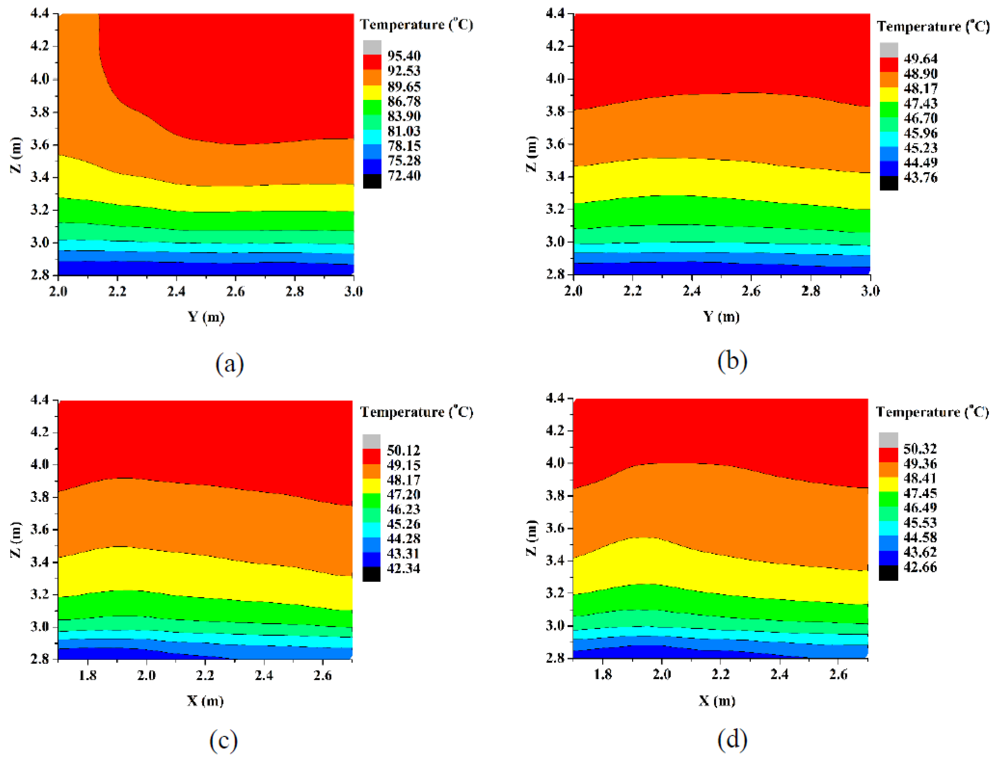
5.3. Temperatures on Each Side of the Shield

The mild steel is applied above the polyethylene layer, preventing the heat from the fire from directly reaching the polyethylene. The density of mild steel is much higher than that of polyethylene, and it takes longer to get heated. The temperature profile of the outer mild steel shield after 400 s is shown in Figure 15. It is observed that the temperature on the mild steel shield does not go above 30 °C for the fire-facing side, i.e., side A, and for the other sides, it is even less than 30 °C. The temperature in the upper part of the shield is higher due to radiation from the hot gases with higher temperatures in the upper layers. When the hot gases descend from the ceiling, they radiate heat, and the temperature goes down for the bottom part of the shield. Additionally, the fresh air supply from the supply vent located on the lower bottom and the removal of hot gases from the exhaust vent located on the above part of the right-side wall results in the uneven temperature distribution on the shield surface. Though the temperature on the four sides of the mild steel does not go beyond 30 °C, the top part of the system (where the mild steel layer does not cover the polyethylene shield) reveals that the unshielded polyethylene layer temperatures do not go beyond 69 °C. The contour for the top part of the shielding is shown in Figure 15d, where the unshielded polyethylene temperature goes to 69 °C. Here, it can also be seen that the mild steel layer’s temperature, however, does not go beyond 50 °C.

Figure 15e illustrates the temperature profile in the top part. The layer with high temperatures (red and grey colored) is the polyethylene shield. It was concluded that though mild steel protects the sides of the polyethylene shield, the upper part still possesses the risk involved as it can withstand much lower heat than mild steel. The next task is to determine the critical time for preventing the polyethylene shield from getting damaged. Additionally, if the polyethylene shield gets damaged (worst-case scenario), what is the extent of its damage? The information on heat transfer in the mild steel and the polyethylene shield is required to determine the scope of the damage. Though the governing equations in FDS yield the temperature predictions by including the conduction mode of heat transfer, these equations are one-dimensional. Thus, they do not account for the overall three-dimensional effects and may lead to over/under predictions. A fully three-dimensional FEM model, COMSOL, was used to avoid uncertainty in the temperature predictions.

The input boundary conditions for COMSOL were obtained from the temperature output for the outer shield predicted by FDS. Thus, a unique coupling methodology was set up wherein FVM based solver, i.e., FDS was used to provide input conditions for solving a conduction-based heat transfer problem more efficiently. The temperatures obtained on each computing node of the sides of the shield were time-averaged over the last 500 s to get a steady state, and this averaged value of temperature was then tabulated for different time scales. The averaged values have been reported in the Supporting Information File.

In the illustrations shown in Figure 16 below, the temperature profile from the FDS simulations after 2400 s. The contours for 800 s and 1600 s can be found in the Supporting Information Section. The temperature profile for 2400 s and the in-between time instances, (i.e., 800 s and 1600 s) follow a similar trend for 400 s. The fire-facing side of the mild steel, i.e., side A, has the highest temperature (30 °C) among the four sides for 400 s. The temperature rises to 47 °C after 800 s, 75 °C after 1600 s, and 98 °C after 2400 s. The shield’s temperature was rising at a much faster rate in the initial stages of the fire growth as the room temperature was rising. Once the entire room got filled with gases, the maximum temperature was reached. After that, the temperature on the shield increased at a slower rate. The other three sides of the mild steel shield had similar temperature ranges for each instance. The temperature on side C had lower temperatures (1–3 °C less than the other two sides). This is because side C is located farther from the fire than the other two sides. In addition, side C is located much closer to the supply vent and was thus exposed to fresh air.

5.4. The Maximum Temperatures on the Shield

The maximum temperatures on each of the five sides of the shield are plotted in Figure 17. It is clear from Figure 17 that the unshielded top of the polyethylene shield has a much higher temperature than the mild steel layers. The difference in the specific heat capacity and thermal conductivity of polyethylene and mild steel results in a faster heating rate of polyethylene.

Furthermore, to estimate the temperature rise in the mild steel shield, three-dimensional conduction heat transfer rates need to be considered, which cannot be done in FDS (FDS assumes heat conduction only in the direction normal to the surface). Obtaining such detailed heat transfer rates required considering a fully three-dimensional energy equation, which is not possible in FDS; it was thus decided to use COMSOL, which has robust heat transfer solving capabilities.

Figure 18a shows that though the temperature of the unshielded polyethylene reaches about 120 °C at 700 s, this high temperature exists only for a depth of ~10 cm. Figure 18b shows that the rise in the temperature is specifically for the polyethylene sheet alone. The temperature inside the SS chamber was found to be around 50 °C. Moreover, the bottom part of polyethylene (sandwiched between the two mild steel layers) has a temperature of less than 50 °C, 700 s after the ignition of the fire.

The simulations carried out at 2400 s illustrated in Figure 18c,d reveal that the top temperature of the polyethylene reaches 167 °C. However, the temperature for the rest of the polyethylene sheet is not greater than 100 °C. Figure 18e,f illustrates that the temperature for the polyethylene shield reaches above its melting point. Additionally, the temperature of mild steel inside the SS chamber has increased to a value of 127 °C.

6. Conclusions

The current study is an effort to develop an efficient and effective methodology for more accurate and reliable enclosure pool fire dynamics simulations involving all three modes of heat transfer (conduction, convection, and radiation). The existing state-of-the-art fire simulation solvers have limitations in modeling the conduction using a one-dimensional equation, which might lack accuracy. A unique coupled finite volume method–finite element method simulation strategy has been proposed and demonstrated to overcome the accuracy issue.

• Firstly, validation and corroboration studies were carried out for simulating methanol pool fires by comparing the results from the present large eddy simulations (carried out in Fire Dynamics Simulator) against experimental results from the literature. The predicted flame heights, centerline temperatures, and velocities are in good agreement with the experimental results.
• The validated mesh configuration was then used for simulating the postulated methanol pool fire scenario. The fire dynamics predicted from FDS were in line with the values obtained from empirical correlations.
• The predicted solid-body temperatures from FDS were used as input boundary conditions for FEM simulations which were then used for carrying out detailed three-dimensional heat transfer simulations to investigate the thermal conduction within the solid (mild steel and polyethylene shields).
• The proposed coupled FVM–FEM technique has been verified and tested in the present study. This technique will be helpful to practicing safety engineers and fire technologists to have a more detailed assessment of pool fires (considering all three modes of heat transfer) which will assist them in the safer design of rooms involving inflammable liquid inventories.

References

1. Vílchez, J.A.; Sevilla, S.; Montiel, H.; Casal, J. Historical Analysis of Accidents in Chemical Plants and in the Transportation of Hazardous Materials. J. Loss Prev. Process Ind. 1995, 8, 87–96. [Google Scholar] [CrossRef]
2. Planas-Cuchi, E.; Montiel, H.; Casal, J. A Survey of the Origin, Type and Consequences of Fire Accidents in Process Plants and in the Transportation of Hazardous Materials. Process Saf. Environ. Prot. 1997, 75, 3–8. [Google Scholar] [CrossRef] [Green Version]
3. Casal Fàbrega, J.; Gómez-Mares, M.; Muñoz, M.Á.; Palacios, A. Jet Fires: A “Minor” Major Accident? Chem. Eng. Trans. 2012, 26, 13–20. [Google Scholar] [CrossRef]
4. Freeman, R.A. CCPS Guidelines for Chemical Process Quantitative Risk Analysis. Plant/Oper. Prog. 1990, 9, 231–235. [Google Scholar] [CrossRef]
5. Sajid, Z.; Khan, M.K.; Rahnama, A.; Moghaddam, F.S.; Vardhan, K.; Kalani, R. Computational Fluid Dynamics (CFD) Modeling and Analysis of Hydrocarbon Vapor Cloud Explosions (VCEs) in Amuay Refinery and Jaipur Plant Using FLACS. Processes 2021, 9, 960. [Google Scholar] [CrossRef]
6. Parihar, R. 12 Dead, over 200 Injured in Indian Oil Depot Fire in Jaipur. Available online: https://www.indiatoday.in/india/story/12-dead-over-200-injured-in-indian-oil-depot-fire-in-jaipur-59623-2009-10-29 (accessed on 22 December 2020).
7. Gai, G.; Cancelliere, P. Design of a Pressurized Smokeproof Enclosure: CFD Analysis and Experimental Tests. Safety 2017, 3, 13. [Google Scholar] [CrossRef] [Green Version]
8. Hehnen, T.; Arnold, L.; La Mendola, S. Numerical Fire Spread Simulation Based on Material Pyrolysis—An Application to the CHRISTIFIRE Phase 1 Horizontal Cable Tray Tests. Fire 2020, 3, 33. [Google Scholar] [CrossRef]
9. Beyler, C.L. Fire hazard calculations for large, open hydrocarbon fires. In SFPE Handbook of Fire Protection Engineering; Hurley, M.J., Gottuk, D., Hall, J.R., Harada, K., Kuligowski, E., Puchovsky, M., Torero, J., Watts, J.M., Wieczorek, C., Eds.; Springer: New York, NY, USA, 2016; pp. 2591–2663. ISBN 978-1-4939-2565-0. [Google Scholar]
10. Ganju, S.; Karanam, A.; Mishra, S.; Saha, N.; Gera, B.; Goyal, P.; Sharma, P.K.; Shelke, A.V. Application of CFD for assessment of containment safety. In Advances of Computational Fluid Dynamics in Nuclear Reactor Design and Safety Assessment; Elsevier: Amsterdam, The Netherlands, 2019; pp. 567–662. [Google Scholar]
11. Sharma, P.K. Modeling of fire with CFD for nuclear power plants (NPPs). In Advances of Computational Fluid Dynamics in Nuclear Reactor Design and Safety Assessment; Woodhead Publishing: Sawston, UK, 2019; pp. 663–727. [Google Scholar]
12. Woo, D.; Seo, J.K. Numerical Validation of the Two-Way Fluid-Structure Interaction Method for Non-Linear Structural Analysis under Fire Conditions. J. Mar. Sci. Eng. 2021, 9, 400. [Google Scholar] [CrossRef]
13. Husain, Z.; Tiwari, S.S.; Pandit, A.B.; Joshi, J.B. Computational Fluid Dynamics Study of Biomass Cook Stove—Part 1: Hydrodynamics and Homogeneous Combustion. Ind. Eng. Chem. Res. 2020, 59, 4161–4176. [Google Scholar] [CrossRef]
14. Husain, Z.; Tiwari, S.S.; Kataria, A.; Mathpati, C.S.; Pandit, A.B.; Joshi, J.B. Computational Fluid Dynamic Study of Biomass Cook Stove—Part 2: Devolatilization and Heterogeneous Combustion. Ind. Eng. Chem. Res. 2020, 59, 14507–14521. [Google Scholar] [CrossRef]
15. Tiwari, M.K.; Gupta, A.; Kumar, R.; Mishra, R.K.; Chaudhary, A.; Sharma, P.K. Experimental Study on Elevated Methanol Pool Fires in a Compartment. Lect. Notes Mech. Eng. 2021, 29, 473–479. [Google Scholar] [CrossRef]
16. Muñoz, M.; Arnaldos, J.; Casal, J.; Planas, E. Analysis of the Geometric and Radiative Characteristics of Hydrocarbon Pool Fires. Combust. Flame 2004, 139, 263–277. [Google Scholar] [CrossRef]
17. Weckman, E.J.; Strong, A.B. Experimental Investigation of the Turbulence Structure of Medium-Scale Methanol Pool Fires. Combust. Flame 1996, 105, 245–266. [Google Scholar] [CrossRef]
18. Chatris, J.M.; Quintela, J.; Folch, J.; Planas, E.; Arnaldos, J.; Casal, J. Experimental Study of Burning Rate in Hydrocarbon Pool Fires. Combust. Flame 2001, 126, 1373–1383. [Google Scholar] [CrossRef]
19. Hamins, A.; Johnsson, E.; Donnelly, M.; Maranghides, A. Energy Balance in a Large Compartment Fire. Fire Saf. J. 2008, 43, 180–188. [Google Scholar] [CrossRef]
20. Mosisa Wako, F.; Pio, G.; Salzano, E. Reduced Combustion Mechanism for Fire with Light Alcohols. Fire 2021, 4, 86. [Google Scholar] [CrossRef]
21. Wen, J.X.; Kang, K.; Donchev, T.; Karwatzki, J.M. Validation of FDS for the Prediction of Medium-Scale Pool Fires. Fire Saf. J. 2007, 42, 127–138. [Google Scholar] [CrossRef]
22. Chun, H.; Wehrstedt, K.-D.; Vela, I.; Schönbucher, A. Thermal Radiation of Di-Tert-Butyl Peroxide Pool Fires—Experimental Investigation and CFD Simulation. J. Hazard. Mater. 2009, 167, 105–113. [Google Scholar] [CrossRef]
23. Chung, W. A CFD Investigation of Turbulent Buoyant Helium Plumes. Master’s Thesis, Applied Science in Mechanical Engineering, University of Waterloo, Waterloo, ON, Canada, 2007. [Google Scholar]
24. Vasanth, S.; Tauseef, S.M.; Abbasi, T.; Abbasi, S.A. Assessment of Four Turbulence Models in Simulation of Large-Scale Pool Fires in the Presence of Wind Using Computational Fluid Dynamics (CFD). J. Loss Prev. Process Ind. 2013, 26, 1071–1084. [Google Scholar] [CrossRef]
25. Tomaskova, M.; Pokorny, J.; Kucera, P.; Balazikova, M.; Marasova, D. Fire Models as a Tool for Evaluation of Energy Balance in Burning Space Relating to Building Structures. Appl. Sci. 2022, 12, 2505. [Google Scholar] [CrossRef]
26. Lenz, S.; Geier, M.; Krafczyk, M. Simulation of Fire with a Gas Kinetic Scheme on Distributed GPGPU Architectures. Computation 2020, 8, 50. [Google Scholar] [CrossRef]
27. Moon, M.-H.; Kim, H.-J.; Min, S.-G.; Kim, S.-C.; Park, W.-J. Simulation of Indoor Fire Dynamics of Residential Buildings with Full-Scale Fire Test. Sustainability 2021, 13, 4897. [Google Scholar] [CrossRef]
28. Salamonowicz, Z.; Krauze, A.; Majder-Lopatka, M.; Dmochowska, A.; Piechota-Polanczyk, A.; Polanczyk, A. Numerical Reconstruction of Hazardous Zones after the Release of Flammable Gases during Industrial Processes. Processes 2021, 9, 307. [Google Scholar] [CrossRef]
29. McGrattan, K.; Hostikka, S.; McDermott, R.; Floyd, J.; Vanella, M.; Weinschenk, C.; Overholt, K. Fire Dynamics Simulator User’s Guide; NIST Special Publication 1019; National Institute of Standards and Technology: Gaithersburg, MD, USA, 2019. [Google Scholar]
30. Fraga, G.C.; Centeno, F.R.; Petry, A.P.; Coelho, P.J.; França, F.H.R. On the Individual Importance of Temperature and Concentration Fluctuations in the Turbulence-Radiation Interaction in Pool Fires. Int. J. Heat Mass Transf. 2019, 136, 1079–1089. [Google Scholar] [CrossRef]
31. Ma, L.; Nmira, F.; Consalvi, J.-L. Large Eddy Simulation of Medium-Scale Methanol Pool Fires—Effects of Pool Boundary Conditions. Combust. Flame 2020, 222, 336–354. [Google Scholar] [CrossRef]
32. Xu, B.; Wen, J. The Effect of Convective Motion within Liquid Fuel on the Mass Burning Rates of Pool Fires—A Numerical Study. Proc. Combust. Inst. 2021, 38, 4979–4986. [Google Scholar] [CrossRef]
33. Yang, D.; Hu, L.H.; Jiang, Y.Q.; Huo, R.; Zhu, S.; Zhao, X.Y. Comparison of FDS Predictions by Different Combustion Models with Measured Data for Enclosure Fires. Fire Saf. J. 2010, 45, 298–313. [Google Scholar] [CrossRef]
34. Vasanth, S.; Tauseef, S.M.; Abbasi, T.; Abbasi, S.A. CFD Simulation of Pool Fires Situated at Differing Elevation. Process Saf. Environ. Prot. 2015, 94, 89–95. [Google Scholar] [CrossRef]
35. Jain, S.; Kumar, S.; Kumar, S.; Sharma, T.P. Numerical Simulation of Fire in a Tunnel: Comparative Study of CFAST and CFX Predictions. Tunn. Undergr. Space Technol. 2008, 23, 160–170. [Google Scholar] [CrossRef]
36. Vasanth, S.; Tauseef, S.M.; Abbasi, T.; Abbasi, S.A. Simulation of Multiple Pool Fires Involving Two Different Fuels. J. Loss Prev. Process Ind. 2017, 48, 289–296. [Google Scholar] [CrossRef]
37. Chen, Z.; Wen, J.; Xu, B.; Dembele, S. Large Eddy Simulation of a Medium-Scale Methanol Pool Fire Using the Extended Eddy Dissipation Concept. Int. J. Heat Mass Transf. 2014, 70, 389–408. [Google Scholar] [CrossRef]
38. Sengupta, A. Optimal Safe Layout of Fuel Storage Tanks Exposed to Pool Fire: One Dimensional Deterministic Modelling Approach. Fire Technol. 2019, 55, 1771–1799. [Google Scholar] [CrossRef]
39. Sengupta, A.; Gupta, A.K.; Mishra, I.M. Engineering Layout of Fuel Tanks in a Tank Farm. J. Loss Prev. Process Ind. 2011, 24, 568–574. [Google Scholar] [CrossRef]
40. Bale, S.; Tiwari, S.; Sathe, M.; Berrouk, A.S.; Nandakumar, K.; Joshi, J. Direct Numerical Simulation Study of End Effects and D/d Ratio on Mass Transfer in Packed Beds. Int. J. Heat Mass Transf. 2018, 127, 234–244. [Google Scholar] [CrossRef]
41. Bale, S.; Tiwari, S.S.; Nandakumar, K.; Joshi, J.B. Effect of Schmidt Number and D/d Ratio on Mass Transfer through Gas-Solid and Liquid-Solid Packed Beds: Direct Numerical Simulations. Powder Technol. 2019, 354, 529–539. [Google Scholar] [CrossRef]
42. Joshi, J.B.; Nandakumar, K.; Patwardhan, A.W.; Nayak, A.K.; Pareek, V.K.; Gumulya, M.M.; Wu, C.; Minocha, N.; Pal, E.; Kumar, M.; et al. Computational fluid dynamics. In Advances of Computational Fluid Dynamics in Nuclear Reactor Design and Safety Assessment; Woodhead Publishing: Cambridge, MA, USA, 2019; pp. 21–238. ISBN 978-0-08-102338-9. [Google Scholar]
43. Tiwari, S.S.; Pal, E.; Bale, S.; Minocha, N.; Patwardhan, A.W.; Nandakumar, K.; Joshi, J.B. Flow Past a Single Stationary Sphere, 1. Experimental and Numerical Techniques. Powder Technol. 2020, 365, 115–148. [Google Scholar] [CrossRef]
44. Tiwari, S.S.; Pal, E.; Bale, S.; Minocha, N.; Patwardhan, A.W.; Nandakumar, K.; Joshi, J.B. Flow Past a Single Stationary Sphere, 2. Regime Mapping and Effect of External Disturbances. Powder Technol. 2020, 365, 215–243. [Google Scholar] [CrossRef]
45. Gajbhiye, B.D.; Kulkarni, H.A.; Tiwari, S.S.; Mathpati, C.S. Teaching Turbulent Flow through Pipe Fittings Using Computational Fluid Dynamics Approach. Eng. Rep. 2020, 2, e12093. [Google Scholar] [CrossRef] [Green Version]
46. Smagorinsky, J. General Circulation Experiments with the Primitive Equations. Mon. Weather Rev. 1963, 91, 99–164. [Google Scholar] [CrossRef]
47. Ghosal, S.; Moin, P. The Basic Equations for the Large Eddy Simulation of Turbulent Flows in Complex Geometry. J. Comput. Phys. 1995, 118, 24–37. [Google Scholar] [CrossRef]
48. Deardorff, J.W. A Numerical Study of Three-Dimensional Turbulent Channel Flow at Large Reynolds Numbers. J. Fluid Mech. 1970, 41, 453–480. [Google Scholar] [CrossRef]
49. Siddapureddy, S.; Wehrstedt, K.-D.; Prabhu, S.V. Heat Transfer to Bodies Engulfed in Di-Tert-Butyl Peroxide Pool Fires—Numerical Simulations. J. Loss Prev. Process Ind. 2016, 44, 204–211. [Google Scholar] [CrossRef]
50. Fernandes Oliveira, R.L.; Doubek, G.; Vianna, S.S.V. On the Behaviour of the Temperature Field around Pool Fires in Controlled Experiment and Numerical Modelling. Process Saf. Environ. Prot. 2019, 123, 358–369. [Google Scholar] [CrossRef]
51. Pio, G.; Carboni, M.; Iannaccone, T.; Cozzani, V.; Salzano, E. Numerical Simulation of Small-Scale Pool Fires of LNG. J. Loss Prev. Process Ind. 2019, 61, 82–88. [Google Scholar] [CrossRef]
52. Ahmadi, O.; Mortazavi, S.B.; Pasdarshahri, H.; Mohabadi, H.A. Consequence Analysis of Large-Scale Pool Fire in Oil Storage Terminal Based on Computational Fluid Dynamic (CFD). Process Saf. Environ. Prot. 2019, 123, 379–389. [Google Scholar] [CrossRef]
53. Drysdale, D. An Introduction to Fire Dynamics; John Wiley & Sons: Hoboken, NJ, USA, 2011. [Google Scholar]
54. Hodgman, C.D. CRC Handbook of Chemistry and Physics; CRC Press: Cleveland, OH, USA, 1978. [Google Scholar]
55. Wood, W. DMIC Report 177: Thermal Radiative Properties of Selected Materials; Battelle Memorial Institute, Defense Metals Information Center: Columbus, OH, USA, 1962. [Google Scholar]
56. Gubareff, G.G.; Janssen, J.E.; Torborg, R.H. Thermal Radiation Properties Survey: A Review of the Literature; Honeywell Research Center, Minneapolis-Honeywell Regulator Company: Minneapolis, MN, USA, 1960. [Google Scholar]
57. Grooshandler, W.L. Radcal—A Narrow-Band Model for Radiation Calculations in a Combustion Environment. 1993. Available online: https://www.govinfo.gov/app/details/https%3A%2F%2Fwww.govinfo.gov%2Fapp%2Fdetails%2FGOVPUB-C13-d0301b96642f0167a45468dd42912cd7 (accessed on 17 April 2022).
58. Hurley, M.J.; Gottuk, D.T.; Hall, J.R., Jr.; Harada, K.; Kuligowski, E.D.; Puchovsky, M.; Torero, J.L.; Watts, J.M., Jr.; Wieczorek, C.J. (Eds.) SFPE Handbook of Fire Protection Engineering, 5th ed.; Springer: New York, NY, USA, 2016. [Google Scholar] [CrossRef]
59. Peatross, M.J.; Beyler, C.L. Ventilation Effects on Compartment Fire Characterization. Fire Saf. Sci. 1997, 5, 403–414. [Google Scholar] [CrossRef] [Green Version]
Figure 1. The schematic diagram for the methanol cleaning system inside an enclosure (a) front view and (b) top view of the cleaning room. The system consists of a methanol pool, an exhaust and supply vent system, and a polyethylene shield (in pink color).
Processes 10 00918 g001
Figure 2. Geometry and mesh for the validation case (a) geometry, and (b) meshing.
Processes 10 00918 g002
Figure 3. Stages of 31 cm methanol pool fire till it attains a steady state.
Processes 10 00918 g003
Figure 4. Average velocity profile for 31 cm methanol pool fire.
Processes 10 00918 g004
Figure 5. Comparison of temperature along horizontal centerlines at heights of (a) 6 cm (b) 12 cm (c) 20 cm above the plume and (d) hot gas layer temperature for different meshes of the present study against experimentally reported values of Weckman and Strong [17] (Experimental data adapted with permission from Weckman and Strong [17]).
Processes 10 00918 g005
Figure 6. Hot gas layer temperature at various elevations along the center of the room.
Processes 10 00918 g006
Figure 7. The temperature along the horizontal centerline at different heights above the plume for the 2 m2 methanol pool fire.
Processes 10 00918 g007
Figure 8. Mean centerline temperature profile for postulated methanol pool.
Processes 10 00918 g008
Figure 9. Incident heat flux on the outer layer of mild steel shield.
Processes 10 00918 g009
Figure 10. Temperature profile on (a) side A (b) side C (c) side B, and (d) side D of polyethylene shield 400 s after ignition of the fire.
Processes 10 00918 g010
Figure 11. The temperature profile of the cleaning system and enclosure (a) from the fire facing side (b) front view fire facing side after 500 s.
Processes 10 00918 g011
Figure 12. Velocity distribution contours plotted on the XZ-center plane.
Processes 10 00918 g012
Figure 13. Oxygen concentration inside the enclosure on the room XZ center plane the (a) after 80 s and (b) after 500 s.
Processes 10 00918 g013
Figure 14. Vertical temperature profile on the XZ center plane (a) after 80 s (b) after 500 s.
Processes 10 00918 g014
Figure 15. Temperature profile on (a) side A (b) side C (c) side B, and (d) side D of mild steel shield and (e) top view of the cleaning system 400 s after ignition of the fire.
Processes 10 00918 g015
Figure 16. Temperature profile on (a) side A (b) side C (c) side B and (d) side D, and (e) top view of the cleaning system after 2400 s.
Processes 10 00918 g016
Figure 17. The temporally evolving maximum temperature along the four sides of the mild steel shield and the unshielded polyethylene.
Processes 10 00918 g017
Figure 18. Temperature profile on (a) center plane and (b) multiple slices along the yz-axis after 800 s; (c) center plane and (d) multiple slices along the yz-axis after 1600 s; (e) center plane and (f) multiple slices along the yz-axis after 2400 s.
Processes 10 00918 g018