Quantitative Method for Liquid Chromatography–Mass Spectrometry Based on Multi-Sliding Window and Noise Estimation

Abstract

LC-MS/MS uses information on the mass peaks and peak areas of samples to conduct quantitative analysis. However, in the detection of clinical samples, the spectrograms of the compounds are interfered with for different reasons, which makes the identification of chromatographic peaks more difficult. Therefore, to improve the chromatographic interference problem, this paper first proposes a multi-window-based signal-to-noise ratio estimation algorithm, which contains the steps of raw data denoising, peak identification, peak area calculation and curve fitting to obtain accurate quantitative analysis results of the samples. Through the chromatographic peak identification of an extracted ion chromatogram of VD2 in an 80 ng/mL standard and the spectral peak identification of data from an open-source database, the identification results show that the algorithm has a better peak detection performance. The accuracy of the quantitative analysis was verified using the LC-HTQ-2020 triple quadrupole mass spectrometer produced by our group for the application of steroid detection in human serum. The results show that the algorithm proposed in this paper can accurately identify the peak information of LC-MS/MS chromatographic peaks, which can effectively improve the accuracy and reproducibility of steroid detection results and meet the requirements of clinical testing applications such as human steroid hormone detection.

1. Introduction

With the continuous development of science and technology, mass spectrometry technology is widely used in analytical chemistry and metrology. Liquid chromatography–tandem mass spectrometry (LC-MS/MS) can greatly improve the ability to analyze complex samples, allowing for highly accurate and sensitive quantitative analysis of substances to meet the needs of clinical analysis [1].

LC-MS/MS uses information on the mass peaks and peak areas of samples to conduct quantitative analysis. However, in the detection of clinical samples, because the ions generated by chromatographic column loss or complex sample matrices interfere with the spectrograms of the compounds to be measured, irregularities in the shapes of peaks can occur, and this makes the identification more difficult, affecting the accuracy of the results [2,3,4,5].

To improve the problem of chromatographic interference in order to obtain accurate quantitative results, many scholars have proposed a variety of methods for peak identification in recent years, and the common methods for chromatographic peak detection mainly include the first-order derivative method, the second-order derivative method and various similar methods derived on this basis [6,7,8]. Parilla P et al. analyzed binary mixtures of folpet and fenamiphos with overlapping chromatographic peaks using the first derivative of the chromatographic detector signal in the time domain [9]. The second derivative of a chromatographic signal can aid in the recognition of composite peaks, but the method has some limitations [10]. Shao et al. applied the wavelet transform to the analysis and quantification of overlapping peaks. The results showed that the chromatographic peak heights of the components extracted from the overlapping signals still had a good linear relationship with their respective concentrations [11,12]. Du et al. proposed the first ridge line peak-finding method using the Mexican cap as the wavelet parent function, which effectively improved the accuracy of mass spectrometry peak identification [13]. Li solved the problem of overlapping peaks using the improved algorithm dynamic particle swarm optimization (DPSO) based on particle swarm optimization (PSO) and reconstructed its single peak [14]. Dromey et al. proposed a deconvolution algorithm for peak type comparison. The deconvolution process entails comparing the mass chromatogram peaks with the model peak and combining the fragment ions of the same peak shape into a mass chromatogram of a compound [15]. The algorithm is more suitable for the identification of almost completely overlapping peaks, but the parameters are more complicated to choose. Zeng et al. used an EMG model to simulate mixed peaks, then used the Fourier deconvolution method to deconvolve the overlapping regions, and finally used a nonlinear least-squares fit to reconstruct the peaks to obtain a single peak [16].

However, the algorithm based on the derivative method has disadvantages in terms of accurate peak identification and is not suitable for commercial applications due to the low operational efficiency of an algorithm based on algorithms with high complexity, such as wavelet variations.

In order to improve the efficiency of chromatographic peak identification and develop a peak identification algorithm suitable for commercial applications, this study proposes a multi-window fast spectral extraction and analysis method based on signal-to-noise ratio estimation and presents an algorithm that forms the steps of raw data denoising, peak identification, peak area calculation and curve fitting so as to obtain accurate quantitative analysis results of the samples to be measured. Based on the LC-HTQ-2020 triple quadrupole mass spectrometer developed by the group, the application of steroid detection in human serum was used as an example to achieve accurate and rapid identification in chromatograms through self-developed quantitative analysis algorithms, thus solving the problem of the inability to accurately quantify clinical samples.

2. Materials and Methods

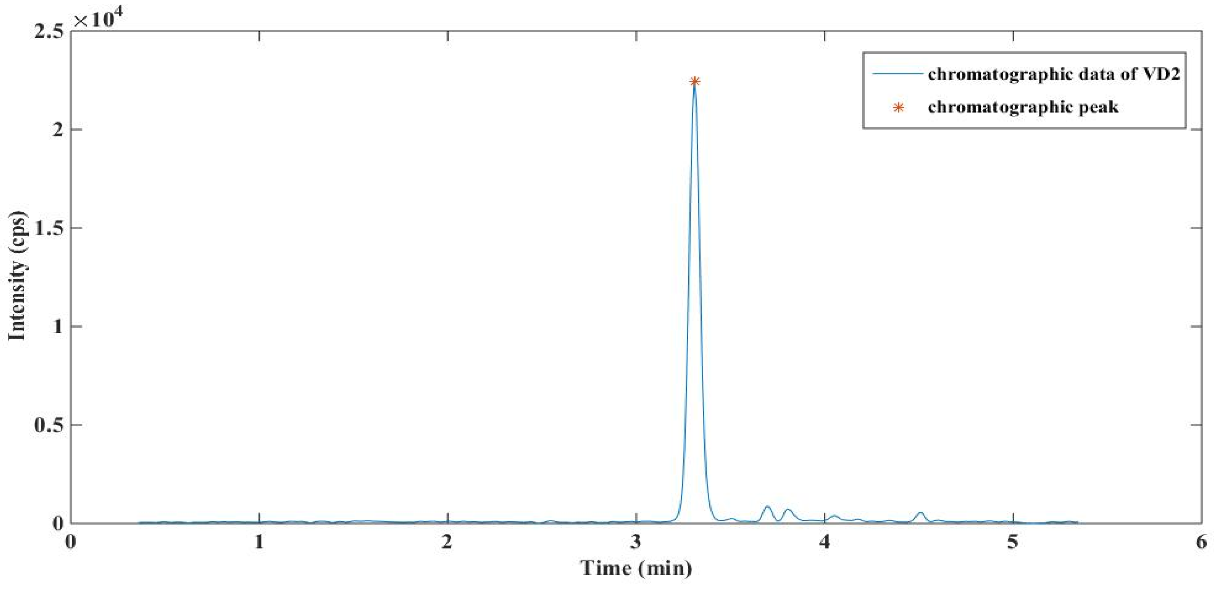
2.1. The Introduction of Chromatographic Signal

The chromatographic signal is the signal–time curve obtained after a certain sample flows through the chromatographic column and detector [14]. The vertical coordinate of a chromatogram generally indicates the magnitude of the signal intensity of the particle with a point, and the horizontal coordinate of the chromatogram indicates the time.

The chromatographic signal can be described as $y\left(t\right)=B\left(t\right)+P\left(t\right)+N\left(t\right)$, where $B\left(t\right)$ is the baseline signal of the chromatogram, $P\left(t\right)$ is the peak signal of the chromatogram and $N\left(t\right)$ is the noise signal.

Normal chromatographic peaks approximate a symmetrically shaped normal distribution curve (Gauss curve). The response signal or differential curve generated when the component to be measured passes through the detector system after flowing from the column is called the chromatographic peak, or simply the peak. Figure 1 shows an example of a chromatographic peak.

The chromatographic peaks have the following characteristics [17,18,19]:

(1)

Peak baseline refers to the distance from the beginning to the end of the peak on the baseline;

(2)

Peak height refers to the height from the highest point of the peak to the baseline of the peak;

(3)

Peak width refers to the distance between the two tangents made at the inflection points on both sides of the peak and the two intersection points of the baseline;

(4)

Half-peak width refers to the width of the peak at half of the peak height.

2.2. Reagents and Instruments

Estrone (E1), estradiol (E2), aldosterone (Ald) and dehydroepiandrosterone sulfate (DHEAS) were supplied by Sigma-Aldrich (Shanghai, China); estriol (E3), 17-hydroxypregnenolone (17-OHPreg) and 17-hydroxypregnenolone-d3 (17-OHPreg-d3) were purchased from Shanghai ZZBIO Co., Ltd. (Shanghai, China); and estrone-d4 (E1-d4), estradiol-d4 (E2-d4), estriol-d3 (E3-d3), aldosterone-d7 (Ald-d7) and dehydroepiandrosterone sulfate-d6 (DHEAS-d6) were obtained from Shanghai Pufen Biotechnology Co., Ltd. (Shanghai, China). HPLC grade methanol and methyl tert-butyl ether (MTBE) were obtained from Tianjin Concord Technology Co., Ltd. (Tianjin, China). Ammonia was purchased from Sinopharm Chemical Reagent Co., Ltd. (Shanghai, China). Charcoal-stripped bovine serum was bought from Zhejiang Tianhang Biotechnology Co., Ltd. (Huzhou, China). The pooled human serum was purchased from Golden West Biologicals (Temecula, CA, USA). Ultrapure water was purified using a UPH-II-20T ultrapure water manufacturing system (Chengdu, China).

The detection of steroids was performed in ESI mode on a liquid chromatography–tandem mass spectrometry system (LC-HTQ-2020) developed by our research group (Tianjin Guoke Medical Engineering and Technology Development Co., Ltd., Tianjin, China).

2.3. Data Processing Algorithm

2.3.1. Data Pre-Processing

The Savitzky–Golay (S-G) filter method is a parameter-free least-squares-based filtering method proposed by Abraham Savitzky and Marcel J. E. Golay in 1964, whose core idea is to weight the data within a window, with the weighting weights obtained by least-squares fitting to a given high-order polynomial [20,21]. The advantage of the filtering method is that it fits the low-frequency signal and smooths out the high-frequency signal while effectively retaining the signal change information.

The filtering process is as follows.

The filter window width (n) is set to 2m + 1, whose data can be expressed as $\left[x_{i-m}, x_{i-m+1}, \dots x_i, \dots x_{i+m-1}, x_{i+m}\right]$. Then, a $k-1$ order polynomial, as shown in Equation (1), is used to fit the measurement points within the filter window.

$$y\left(i\right)={{\displaystyle \sum }}_{b=0}^{k-1}{a}_b{i}^b$$

(1)

where $a_b$ (b = 0, 1, 2, …, $k-1$) is the fitting coefficient, k is the polynomial order, and $y\left(i\right)$ is a polynomial of order $k-1$ to fit the data points. The residual can be calculated using Equation (2).

$${\epsilon }_i={{\displaystyle \sum }}_{i=-m}^m{\left(y\left(i\right)-x_i\right)}^2={{\displaystyle \sum }}_{i=-m}^m{({{\displaystyle \sum }}_{b=0}^{k-1}{a}_b{i}^b-x_i)}^2$$

(2)

When all partial derivatives with respect to $a_n$ are zero, the residual takes the minimum value. Through the above steps, n equations can be obtained, forming a system of $k$-element linear equations, as shown in Equation (3), and the fitting parameters can be determined by least-squares fitting.

$$\left(\begin{array}{c}{y}_{-m}\\ y_{-m-1}\\ ⋮\\ y_{m-1}\\ y_m\end{array}\right)=\left(\begin{array}{cccc}1& -m& \cdots & {\left(-m\right)}^{k-1}\\ 1& -m+1& \cdots & {\left(-m+1\right)}^{k-1}\\ ⋮& ⋮& ⋮& ⋮\\ 1& m& \cdots & m^{k-1}\end{array}\right)\left(\begin{array}{c}{a}_0\\ a_1\\ ⋮\\ a_{k-1}\end{array}\right)+\left(\begin{array}{c}{\epsilon }_{-m}\\ {\epsilon }_{-m+1}\\ ⋮\\ {\epsilon }_m\end{array}\right)$$

(3)

Equation (3) can be expressed as the following matrix.

$$Y_{(2m+1)\times 1}=X_{(2m+1)\times k}{A}_{k\times 1}+E_{(2m+1)\times 1}$$

(4)

where X is the data matrix, A is the fitted parameter matrix, E is the residual matrix, and Y is the corresponding polynomial matrix. The corresponding subscripts are the dimensions of the respective matrices. The least-squares solution of matrix $\hat{A}$ can be calculated from Equation (5).

$$\hat{A}={\left(X^{T}X\right)}^{-1}{X}^{T}Y$$

(5)

The filtered data can be expressed as Equation (6), where B is the auxiliary matrix, which is the relationship matrix between the filtered values and the observed values.

$$\hat{Y}=XA=\left(X^{T}X\right){}^{-1}{X}^{T}Y=BY$$

(6)

2.3.2. Signal-to-Noise Ratio Estimation Algorithm Based on Histogram Statistics

For LC-MS/MS data, S/N is the ratio of the real signal of the chromatogram to the noise under a certain definition [22,23,24]. Because the chromatographic signal obtained is the combination of noise and the real signal, the histogram-statistics-based S/N estimation method is proposed to estimate the S/N of each data point in the chromatogram.

First, the expectation $E\left(X\right)$ and standard deviation $STDEV$ (X) of all data in the chromatogram are calculated, where X denotes the vector of chromatogram data composition. The threshold $IN{S}_{MAX}$ can be expressed as Equation (7).

$$IN{S}_{MAX}=E\left(X\right)+\eta STDEV\left(X\right)$$

(7)

where $\eta$ can be selected according to the requirements, and its empirical value is 3. The number of boxes of the histogram is set to $N_{bin}$ with an empirical value of 30. The histogram can be divided into $N_{bin}$ segments, and the length of each segment is $IN{S}_{SIZE}$.

$$IN{S}_{SIZE}=\frac{IN{S}_{MAX}}{N_{bin}}$$

(8)

The segments of the histogram are $[0,IN{S}_{SIZE})$, $[IN{S}_{SIZE},2IN{S}_{SIZE})$, ……, $[\left(N_{bin}-1\right)IN{S}_{SIZE},N_{bin}IN{S}_{SIZE})$. The data in the chromatogram that exceed $IN{S}_{MAX}$ are ignored, and data smaller than $IN{S}_{MAX}$ are counted in a segment of the histogram. The $N_{bin}$ segments are arranged according to the number of data falling into them; the median number of data is $[\left(N_m-1\right)IN{S}_{SIZE},N_{m}IN{S}_{SIZE})$, and then the estimated noise n is $n=\left(N_m-0.5\right)IN{S}_{SIZE}$.

Because the noise should in principle be greater than or equal to 1, the noise is corrected using Equation (9).

$$n=\max \left\{1,\left(N_m-0.5\right)IN{S}_{SIZE}\right\}$$

(9)

The estimated signal-to-noise ratio of the data is calculated using Equation (10).

$$y{n}_t=y\left(t\right)/n$$

(10)

2.3.3. A Multi-Sliding Window Peak Identification Algorithm

The algorithm uses multiple fixed-size sliding windows to calculate the mean and standard deviation of a certain number of data to classify the peak points, which is detailed in

Table 1. The data process of the multi-sliding window peak identification algorithm.

Step	Data Process
1	Input: SmoothData y, threshold n. peak threshold n1
2	Logarithm of SmoothData X = log(y)
3	Calculate the mean avg and standard deviation std in a large sliding window whose window length is m. Calculate the flags of all data. For each yi    If log(yi) − avg > n∗std, flagi = 1;    If log(yi) − avg < n∗std, flagi = −1; Otherwise flagi = 0; If flagi ≠ 1, the window slides forward one point, repeat step 3.
4	For each flagi    If flagi = 1, the variable peakstart is i − 1; set Sstart = i − 1;    If flagi ≠ 1, flagi+1 ≠ 1, and peakstart ! = null, peakstart = null; set Send = i; In the range from Sstart to Send, MWPeakswindow1.Intenstity = max[ySstart,ySend], MWPeakswindow1.peakpoint = the time corresponding to the maximum value.
5	Define a small sliding window whose window length is m1, repeat the steps of 3–5. The information of MWPeakswindow2 can be obtained.
6	Combine MWPeakswindow1 and MWPeakswindow2 into MWPeaks. Remove the duplicate peaks in MWPeaks.
7	Combine MWPeakswindow1 and MWPeakswindow2 into MWPeaks. Remove the duplicate peaks in MWPeaks.
8	For each MWPeaks If MWPeaks[i]. Intenstity < n1, delete the peak.
9	Output: set of peaks MWPeaks

. However, taking into account that the signal fluctuation range is large, in order to avoid the mean and standard deviation of the peak data, the intensities of the original data are logarithmically transformed to reduce fluctuations in the signal intensity values, pre-processed data X are obtained, and then data processing is performed.

The first sliding window length is set to m, and then the mean value (avg) and standard deviation (std) of the sliding window are calculated. Then, the threshold is set to n, and the signal strength fluctuation range value is n∗std. According to this fluctuation range, the signal type can be classified. The signal classification process is as follows.

(1)

For each datum X_i of the sliding window, $\Delta x$ is calculated as $\log \left(X_i\right)-avg$.

(2)

If $\Delta x$ is larger than n∗std, X_i can be classified as the part of the peak area, and the flag of X_i is set to 1.

(3)

If $\Delta x$ is smaller than n∗std, X_i can be classified as the part of the peak valley, and the flag of X_i is set to −1.

(4)

If $\Delta x$ is within n*std, X_i can be classified as the normal signal, and the flag of X_i is set to 0.

If the flag of X_i is not equal to 1, the window starts sliding forward, then avg and std within that window are recalculated, and the above process is repeated until all data are completed. Figure 2 shows the partial results of the peaks identified using the above data process and the corresponding chromatographic peak information of VD2 in a 20 ng/mL standard. In Figure 2a, the algorithm identifies the chromatographic data from 1.722 to 3.329 min as the region of peak occurrence. In Figure 2b, it can be seen that the chromatographic peak appears at 3.182 min and is correctly identified by the algorithm, which is consistent with the algorithm recognition results. These results show that the peak regions are effectively extracted, and the algorithm has a good performance for chromatographic peak identification.

After a set flag of the flags of all data is obtained, the peak point of each peak area can be searched using the following steps.

(1)

The peak threshold is input to filter all mass spectral peaks with peaks greater than the threshold.

(2)

If Flag_i = 1, we determine the previous point of the data point as the peak starting point S_start and define a variable peak_start that stores the point’s position.

(3)

If Flag_i ≠ 1, Flag_i+1 ≠ 1, and peak_start is non-empty, we determine the point as the peak end point S_end and set the peak_start to empty.

(4)

In the range of S_start to S_end, we find the position of the data point with the highest intensity, that is, the peak point.

(5)

The intensity of the peak point is compared with the threshold; if it is greater than the threshold, the peak information can be output.

(6)

The above process is repeated until the completion of the search for all peaks.

Then, we use another sliding window with the length m1 and repeat the above steps to complete the search for all peaks. We remove duplicate peaks and store the peak information obtained from the two windows in the set MWPeaks.

2.3.4. Multi-Window-Based Signal-to-Noise Ratio Estimation Algorithm

The quantitative analysis of LC-MS/MS is generally based on the peak area as the quantitative standard, so it needs to identify the boundaries of the peak. In this paper, we first propose a multi-window-based signal-to-noise ratio estimation algorithm, which can identify the peak area well and lay the foundation for the accuracy of quantitative analysis.

Figure 3 illustrates the data process of the algorithm in this paper. The raw chromatographic data obtained by LC-MS/MS are filtered by the S-G filter detailed in Section 2.3.1 to remove high-frequency signals, then the peak points are identified using the multi-window peak identification algorithm proposed in Section 2.3.3 and stored in the MWPeaks set, and then the signal-to-noise ratio estimation algorithm based on histogram statistics proposed in Section 2.3.2 is used to calculate the S/N ratio of each data point. For each peak in MWPeaks, according to the set S/N ratio threshold, the algorithm traverses the data on the left and right sides of the peak point until the S/N ratio of a certain data point is less than the threshold. The algorithm considers the two data points as the left and right boundaries of the corresponding peak. Then, the algorithm compares the peak width to exclude peaks whose width is less than the set value. The peak boundaries and the corresponding peak point are stored in the MWPeaks set.

At last, the algorithm calculates the peak area of each peak by Equation (11) for quantitative analysis. We define the peak area as $S_{peak}=S_{all}-S_H$, $S_{all}$, which can be approximated as the number of trapezoidal areas.

$$S_{all}={\displaystyle \sum }_{x=1}^n\frac{1}{2}\left(f\left(x\right)+f\left(x+1\right)\right)·\Delta x$$

(11)

The noise area $S_H$ is $\frac{1}{2}\left(f\left(1\right)+f\left(n\right)\right)·n$.

The peak information MWPeaks, which contains peak points, peak boundaries and peak area, is used for later quantitative information, which is detailed in Section 2.3.5.

2.3.5. Quantitative Analysis Method

Common methods of LC-MS/MS quantitative analysis include the external standard method and internal standard method. The internal standard method is a more accurate quantitative method in chromatographic analysis; especially when there is no standard control, this method is far superior.

The process of the internal standard method includes the preparation of samples, chromatographic analysis and quantitative analysis [23]. The samples contain an internal standard with a known concentration and a certain number of components being analyzed. Then, the samples are introduced into the LC-MS/MS system to perform chromatographic analysis. In the quantitative analysis of the peak area (or peak height) of the internal standard and the component to be measured, a calibration equation can be calculated by the multi-window-based signal-to-noise ratio estimation algorithm, and the percentage content of the component with an unknown concentration can be calculated by the calibration equation.

The main function of this method is to quantify the relationship between analyte concentration and area ratio. The steps of the internal standard method for LC-MS/MS quantitative analysis are shown in Figure 4.

In Figure 4, the multi-window-based signal-to-noise ratio estimation algorithm is used to identify the maximum peak area value of each spectrum for each sample in a specified time period, and then the corresponding analyte peak area is divided by the internal standard peak area. For any one substance, two sets of variable values can be obtained, one for the concentration of the analyte (X) and the other for the ratio of the analyte peak area to the internal standard peak area (Y). Assuming that the variables X and Y obey the linear function $y=bx+a$, which is called the calibration equation, where the parameters a and b are calculated using weighted least-squares estimation based on the available sample values [24,25], then the other unknown samples’ concentrations can be calculated by the calibration equation.

2.4. Steroid Analysis

2.4.1. Calibration Samples

A combined standard solution was prepared from stock solutions of standards by dilution with methanol. The calibration solution was obtained by adding a combined standard solution to surrogate matrix charcoal-stripped bovine serum. The concentrations of the calibrators of E1 were 0.02 ng/mL, 0.05 ng/mL, 0.1 ng/mL, 0.2 ng/mL, 0.5 ng/mL, 1 ng/mL, 1.5 ng/mL and 2 ng/mL; those of E2 were 0.05 ng/mL, 0.1 ng/mL, 0.2 ng/mL, 0.5 ng/mL, 0.8 ng/mL, 1 ng/mL, 1.5 ng/mL and 2 ng/mL; those of E3 were 0.1 ng/mL, 0.5 ng/mL, 1 ng/mL, 2 ng/mL, 5 ng/mL, 10 ng/mL, 25 ng/mL and 50 ng/mL; those of 17-OHPreg were 0.5 ng/mL, 1 ng/mL, 2 ng/mL, 5 ng/mL, 10 ng/ mL, 50 ng/mL, 100 ng/mL and 200 ng/mL; those of Ald were 0.1 ng/mL, 0.25 ng/mL, 0.5 ng/mL, 0.75 ng/mL, 1 ng/mL, 2.5 ng/mL, 5 ng/mL and 10 ng/mL, and those of DHEAS were 10 ng/mL, 50 ng/mL, 50 ng/mL and 10 ng/mL, respectively.

The combined internal standard (IS) working solution was also prepared from the corresponding stock solutions by dilution with methanol. The concentrations of E1-d4, E2-d4, E3-d3, 17-OHPreg-d3, Ald-d7 and DHEAS-d6 were 15 ng/mL, 50 ng/mL, 200 ng/mL, 1 μg/mL, 60 ng/mL and 20 μg/mL, respectively.

2.4.2. Liquid Chromatography–Tandem Mass Spectrometry Conditions

Liquid chromatographic conditions were set up as follows. Chromatographic separation was performed on a Durashell C18 (L) column (3.0 × 50 mm, 3 µm, 150 Å) from Agela Technologies. The mobile phases were 0.1% aqueous ammonia solution (phase A) and methanol (phase B). Gradient elution was performed as follows: 0–1.6 min, 15% B; 1.6–1.8 min, 95% B; 1.8–3.6 min, 95% B; 3.6–3.7 min, 15% B; and 3.7–5.0 min, 15% B. The flow rate was 0.6 mL/min, the sample injection volume was 20 µL, and the column oven temperature was 40 °C.

Tandem mass spectrometry conditions were as follows. The detection was carried out using multiple reaction monitoring (MRM) in negative ion mode. The pressure of curtain gas (CUR) was 30 psi, that of nebulizer (GS1) was 50 psi, that of auxiliary heating gas (GS2) was 60 psi, and that of collision gas (CAD) was 10 psi. The ion source temperature (TEM) was 500 °C, and ionization voltage (IS) was set to −4500 V. The specific mass spectrometry parameters for each compound, such as parent ion, daughter ion, retention time (RT), cone hole voltage and collision energy, are shown in

Table 2. Mass spectrometric acquisition parameters.

Compound	Retention Time (min)	Precursor (m/z)	Quantifier (m/z)	DP (V)	CE (V)
E1	3.50	269.0	145.1	−100	−50
E1-d4	3.49	273.1	147.1	−120	−55
E2	3.49	271.0	145.1	−120	−57
E2-d4	3.48	275.1	147.1	−120	−58
E3	3.27	287.1	171.1	−120	−52
E3-d3	3.27	290.1	173.1	−125	−53
17-OHPreg	3.56	331.1	287.2	−80	−27
17-OHPreg-d3	3.56	334.1	287.2	−80	−28
Ald	3.30	359.1	189.0	−78	−25
Ald-d7	3.29	366.1	194.1	−80	−27
DHEAS	3.08	367.1	97.0	−100	−25
DHEAS-d6	3.08	373.1	98.0	−100	−20

.

2.4.3. Sample Preparation

First, 500 μL samples were added to 2.0 mL microfuge tubes, followed by 10 μL of IS working solution. Then, 1000 μL of MTBE was used as the extractant and added to the samples. The tubes were centrifuged at 14,000× g for 5 min after vigorous shaking. Then, 900 μL of supernatant was transferred from the fully layered solution, and the solvent was removed by nitrogen blowing. The samples were redissolved in 80 μL of methanol/water (50/50, v/v) and placed into the autosampler of the LC-MS/MS system.

2.4.4. Method Validation

To determine the lower limit of quantification (LLOQ), 10 replicates of samples with set concentrations were measured, and the accuracy and coefficient of variation (CV) of the test results were calculated. Recoveries were determined by analyzing blank and spiked samples prepared from the commercial pooled human serum. For each selected level, 5 replicates of samples were processed and quantified. To evaluate the repetitiveness of the method, low-, medium- and high-concentration samples were selected for a precision test. The precision test for each analyte comprised 3 independent analytical runs, and each run comprised 6 replicates of samples. The intra-batch precision and inter-batch precision, as well as the total precision of each concentration of the sample, were evaluated, respectively.

3. Results

3.1. Analysis of Spectral Peak Identification

In this paper, a multi-window peak identification algorithm based on the signal-to-noise ratio is proposed. The algorithm can be applied not only to the identification of chromatographic peaks but also to other peaks’ identification, such as mass spectral peaks.

Figure 5 shows the extracted ion chromatogram of Vitamin D2 (VD2) in an 80 ng/mL standard and the identification result of VD2 chromatographic peaks. As can be seen in Figure 4, the retention time of VD2 is about 3.080 min, and the chromatographic peak of VD2 is correctly identified. The results show that the algorithm has a better identification performance for chromatographic peak identification.

To verify the usability of the algorithm applied to the identification of other peaks, such as mass spectral peaks, we performed a peak recognition algorithm test using a publicly available dataset, which was downloaded from Public Datasets (mdanderson.org) and was obtained based on the simulation of the mathematical model proposed by Morris et al. [26,27]. The publicly available dataset contains a set of mass spectral data and the real peak position information, which is widely used for the comparison of different spectral peak detection methods. The comparison results are shown in Figure 6.

In the figure, it can be seen that the algorithm proposed in this paper identified most of the peaks, which are close to the real peak data, verifying the accuracy of the algorithm and laying the foundation for the subsequent quantitative analysis.

3.2. Methodological Examination

To verify the accuracy of the quantitative analysis, the LC-HTQ-2020 triple quadrupole mass spectrometer, an instrument developed by our group, was used to collect the real data for accuracy testing.

3.2.1. Lower Limit of Quantification (LLOQ)

Based on the clinical testing requirements of E1, E2, E3, 17-OHPreg, Ald and DHEAS and the sensitivity of the instrumentation, the LLOQ of the method was set at 0.02 ng/mL for E1, 0.05 ng/mL for E2, 0.1 ng/mL for E3, 0.5 ng/mL for 17-OHPreg, 0.1 ng/mL for Ald and 0.1 ng/mL 10 ng/mL for DHEAS. All compounds were tested in 10 consecutive tests, and the deviation between the test value and the theoretical value, as well as the CV value of the coefficient of variation of the test results, was calculated. The calculated results are shown in

Table 3. Linear range, correlation coefficient and LLOQ of different compounds.

Compound	Linear Range (ng/mL)	Correlation Coefficient (r2)	Regression Equation y = ax + b	LLOQ (ng/mL)	Recovery (%)	Precision (CV%)
E1	0.02–2.00	0.9988	y = 4.79200x + 0.06490	0.02	97.91	7.96
E2	0.05–2.00	0.9952	y = 2.21100x − 0.04550	0.05	94.60	5.20
E3	0.10–50.00	0.9958	y = 0.43900x + 0.20800	0.10	102.70	8.61
17-OHPreg	0.50–200.00	0.9998	y = 0.09930x + 0.00454	0.50	100.42	7.06
Ald	0.10–10.00	0.9954	y = 2.24200x − 0.33100	0.10	102.70	7.82
DHEAS	10.00–5000.00	0.9998	y = 0.00386x − 0.04550	10.00	99.12	7.43

.

As shown in Table 3, the correlation coefficients of each compound are between 0.9952 and 0.9998, showing good linearity, and the LLOQs are calculated as 0.02~10.00 ng/mL, which are compliant with the linear range of the corresponding compound. The deviations between the tested and theoretical values of LLOQ samples are within 15%. The recoveries of these compounds are 94.60~102.70% with CVs less than 20%.

The results in Table 3 show that the set of LLOQs of each compound meets the standard of clinical assay methodology, showing the accuracy of the algorithm in this paper.

3.2.2. Recovery

The calculated results for three selected levels (i.e., low level, medium level and high level) are listed in

Table 4. The results of recoveries of different compounds.

Compound		Low Level (n = 5)			Medium Level (n = 5)			High Level (n = 5)
	Spike (ng/mL)	Test (ng/mL)	Recovery (%)	Spike (ng/mL)	Test (ng/mL)	Recovery (%)	Spike (ng/mL)	Test (ng/mL)	Recovery (%)
E1	0.05	0.046	92.49	0.50	0.536	107.13	1.50	1.65	110.03
E2	0.10	0.102	102.15	0.80	0.815	101.82	1.50	1.628	108.51
E3	0.50	0.54	107.40	5.00	4.410	88.20	25.00	23.10	92.41
17-OHPreg	1.00	1.29	110.35	10.00	10.310	101.27	100.00	102.65	102.46
Ald	0.25	0.28	110.28	1.00	1.050	105.38	5.00	4.71	94.23
DHEAS	50.00	48.12	96.25	500.00	469.420	93.88	2500.00	2656.60	106.26

. It can be seen that the recoveries range from 88.20% to 110.35%, and the deviation between the detection value and the theoretical value is within ±15%, proving that the method is reliable for the accurate quantification of steroids in human serum.

3.2.3. Precision

The precisions determined using the three levels of samples are listed in

Table 5. Within-run and between-run CVs of different compounds.

Compound	Low Concentration			Medium Concentration			High Concentration
	CV Intra (%)	CV Inter (%)	CV Overall (%)	CV Intra (%)	CV Inter (%)	CV Overall (%)	CV Intra (%)	CV Inter (%)	CV Overall (%)
E1	8.75	3.43	7.62	8.39	4.78	8.30	8.10	3.94	7.36
E2	7.65	0.34	7.24	6.65	2.08	6.13	8.40	2.16	5.91
E3	8.70	2.20	7.74	5.41	2.07	4.37	5.10	1.15	4.15
17-OHPreg	9.56	8.44	9.33	7.77	7.85	8.32	9.82	11.51	11.53
Ald	9.24	1.06	7.38	7.70	2.52	7.34	6.99	4.83	7.07
DHEAS	4.19	0.10	3.44	4.95	1.45	3.91	4.01	0.71	3.46

. For the six kinds of target analytes (E1, E2, E3, 17-OHPreg, Ald and DHEAS), the CV% values of intra-batch precision, inter-batch precision and total precision of the three concentrations are within 15%, indicating the excellent repeatability and meeting the requirement of method validation.

4. Discussion

This paper first proposes a multi-window-based signal-to-noise ratio estimation algorithm to identify chromatographic peaks. Through several experiments, it was found that the algorithm can be applied not only to the identification of chromatographic peaks but also to other peaks’ identification, such as mass spectral peaks.

For the identification of chromatographic peaks, the algorithm can correctly classify chromatographic peaks. A steroid detection test was performed, and the results of the lower limit of quantification (LLOQ), the recovery of different compounds and within-run and between-run CVs of different compounds showed the accuracy of the algorithm, which meets the requirements of clinical testing applications, such as detecting human steroid hormones. This algorithm can be used in the quantitative analysis of LC-MS/MS.

For the identification of mass spectral peaks, the algorithm shows a good peak identification performance, but there is a problem of too high a recognition sensitivity, which can cause some false peaks. For example, in Figure 6, there is the problem of the mismatch between the peaks identified in this paper compared with the real peak position data. The reason for the peak mismatch (such as the peak shift and loss) may be due to the fact that the algorithm identifies the filtered mass spectral data, and the real peak data are based on the original data. After filtering, the filtered data are slightly different from the original data, with differences such as changes in intensity. Some peaks with a low intensity may be filtered out, and they cannot be classified by the multi-window-based signal-to-noise ratio estimation algorithm, causing the peak loss phenomenon. In addition, in Figure 6, some interfering peaks with low signal intensity are also mistaken as real peaks because of the excessively high recognition sensitivity. In future research, the algorithm will be improved to more correctly identify mass spectral peaks and decrease false peaks, laying the foundation for qualitative analysis.

5. Conclusions

This paper proposes a multi-window-based signal-to-noise ratio estimation algorithm for the identification of chromatographic peaks, achieving accurate quantitative analysis of clinical samples. The algorithm includes the steps of raw data denoising, peak identification, peak area calculation and curve fitting. According to experimental verification, the algorithm proposed in this paper can accurately identify the peak information of LC-MS/MS chromatographic peaks, but it identifies not only chromatographic peaks but also mass spectral peaks, etc. In addition, the algorithm can effectively improve the accuracy and repeatability of steroid detection results and can meet the requirements of human steroid hormone detection and other clinical testing applications.

References

1. Wu, A.H.B.; French, D. Implementation of liquid chromatography/mass spectrometry into the clinical laboratory. Clin. Chim. Acta 2013, 420, 4–10. [Google Scholar] [CrossRef] [PubMed]
2. Nielen, M.W.F.; Hooijerink, H.; Zomer, P.; Mol, J.G.J. Desorption electrospray ionization mass spectrometry in the analysis of chemical food contaminants in food. TrAC Trends Anal. Chem. 2011, 30, 165–180. [Google Scholar] [CrossRef]
3. Yang, Y.; Liang, Y.S.; Yang, J.N.; Ye, F.Y.; Zhou, T.; Li, G.K. Advances of supercritical fluid chromatography in lipid profiling. J. Pharm. Anal. 2019, 9, 1–8. [Google Scholar] [CrossRef] [PubMed]
4. Bos, T.S.; Knol, W.C.; Molenaar, S.R.A.; Niezen, L.E.; Schoenmakers, P.J.; Somsen, G.W.; Pirok, B.W.J. Recent applications of chemometrics in one- and two-dimensional chromatography. J. Sep. Sci. 2020, 43, 1678–1727. [Google Scholar] [CrossRef] [PubMed]
5. Lin, J.S.; Liu, X.F.; Wang, J.; Li, D.; Zhu, W.Q.; Chen, W.B.; Zhang, X.H.; Li, Q.M.; Li, M. An artifactual solution degradant of pregabalin due to adduct formation with acetonitrile catalyzed by alkaline impurities during HPLC sample preparation. J. Pharm. Biomed. Anal. 2019, 175, 7. [Google Scholar] [CrossRef]
6. Zhang, Z.M.; Tong, X.; Peng, Y.; Ma, P.; Zhang, M.J.; Lu, H.M.; Chen, X.Q.; Liang, Y.Z. Multiscale peak detection in wavelet space. Analyst 2015, 140, 7955–7964. [Google Scholar] [CrossRef]
7. Wei, X.L.; Shi, X.; Kim, S.; Patrick, J.S.; Binkley, J.; Kong, M.Y.; McClain, C.; Zhang, X. Data dependent peak model based spectrum deconvolution for analysis of high resolution LC-MS data. Anal. Chem. 2014, 86, 2156–2165. [Google Scholar] [CrossRef]
8. Li, B.Q.; Siu, S.; Evans, J.W. Microcomputer processing of chromatographic data. J. Chromatogr. Sci. 1987, 25, 281–285. [Google Scholar] [CrossRef]
9. Parilla, P.; Galera, M.M.; Vidal, J.M.; Frenich, A.G. Determination of fenamiphos and folpet in water by time-domain differentiation of high-performance liquid chromatographic peaks. Analyst 1994, 119, 2231–2236. [Google Scholar] [CrossRef]
10. Asnin, L.D. Peak measurement and calibration in chromatographic analysis. TrAC Trends Anal. Chem. 2016, 81, 51–62. [Google Scholar] [CrossRef]
11. Shao, X.; Cai, W.; Sun, P. Determination of the component number in overlapping multicomponent chromatogram using wavelet transform. Chemom. Intell. Lab. Syst. 1998, 43, 147–155. [Google Scholar] [CrossRef]
12. Dinç, E.; Komsta, Ł.; Vander Heyden, Y.; Sherma, J. Chemometric strategies in chromatographic analysis of pharmaceuticals. Chemom. Chromatogr. 2018, 95, 381–414. [Google Scholar]
13. Du, P.; Kibbe, W.A.; Lin, S.M. Improved peak detection in mass spectrum by incorporating continuous wavelet transform-based pattern matching. Bioinformatics 2006, 22, 2059–2065. [Google Scholar] [CrossRef] [PubMed] [Green Version]
14. Li, Y. Dynamic particle swarm optimization algorithm for resolution of overlapping chromatograms. In Proceedings of the 2009 Fifth International Conference on Natural Computation, Tianjin, China, 14–16 August 2009; pp. 246–250. [Google Scholar]
15. Dromey, R.G.; Stefik, M.J.; Rindfleisch, T.C.; Duffield, A.M. Extraction of mass spectra free of background and neighboring component contributions from gas chromatography/mass spectrometry. Anal. Chem. 1976, 48, 1368–1375. [Google Scholar] [CrossRef]
16. Zeng, Z.D.; Chin, S.T.; Hugel, H.M.; Marriotta, P.J. Simultaneous deconvolution and re-construction of primary and secondary overlapping peak clusters in comprehensive two-dimensional gas chromatography. J. Chromatogr. A 2011, 1218, 2301–2310. [Google Scholar] [CrossRef]
17. Grushka, E. Chromatographic peak capacity and the factors influencing it. Anal. Chem. 1970, 42, 1142–1147. [Google Scholar] [CrossRef]
18. Sorensen, M. Ultrahigh Pressure Capillary Liquid Chromatography-Mass Spectrometry for Metabolomics and Lipidomics. Ph.D. Thesis, University of Michigan, Ann Arbor, MI, USA, 2021. [Google Scholar]
19. Foley, J. Equations for chromatographic peak modeling and calculation of peak area. Anal. Chem. 1987, 59, 1984–1987. [Google Scholar] [CrossRef]
20. Roy, I.G. An optimal Savitzky–Golay derivative filter with geophysical applications: An example of self-potential data. Geophys. Prospect. 2020, 68, 1041–1056. [Google Scholar] [CrossRef]
21. Ruffin, C.; King, R.L. The analysis of hyperspectral data using Savitzky-Golay filtering-theoretical basis. In Proceedings of the IEEE 1999 International Geoscience and Remote Sensing Symposium, IGARSS’99 (Cat. No.99CH36293), Hamburg, Germany, 28 June–2 July 1999; Volume 752, pp. 756–758. [Google Scholar]
22. Zhang, Z.; McElvain, J.S. Optimizing spectroscopic signal-to-noise ratio in analysis of data collected by a chromatographic/spectroscopic system. Anal. Chem. 1999, 71, 39–45. [Google Scholar] [CrossRef]
23. Tautenhahn, R. Feature-Detektion, Annotation und Alignment von Metabolomik LC-MS Daten. Ph.D. Thesis, Martin-Luther-Universität Halle-Wittenberg, Halle, Germany, 2009. [Google Scholar]
24. Rebentrost, P.; Mohseni, M.; Lloyd, S. Quantum support vector machine for big data classification. Phys. Rev. Lett. 2014, 113, 130503. [Google Scholar] [CrossRef]
25. Tan, A.; Lévesque, I.A.; Lévesque, I.M.; Viel, F.; Boudreau, N.; Lévesque, A. Analyte and internal standard cross signal contributions and their impact on quantitation in LC–MS based bioanalysis. J. Chromatogr. B 2011, 879, 1954–1960. [Google Scholar] [CrossRef] [PubMed]
26. Morris, J.S.; Coombes, K.R.; Koomen, J.; Baggerly, K.A.; Kobayashi, R. Feature extraction and quantification for mass spectrometry in biomedical applications using the mean spectrum. Bioinformatics 2005, 21, 1764–1775. [Google Scholar] [CrossRef] [PubMed] [Green Version]
27. Carmona, R.A.; Hwang, W.L.; Torresani, B. Multiridge detection and time-frequency reconstruction. IEEE Trans. Signal Processing 2015, 47, 492. [Google Scholar] [CrossRef] [Green Version]
Figure 1. An example of a chromatographic signal.
Processes 10 01098 g001
Figure 2. An example of the signal classification results of the extracted ion chromatogram of VD2 in a 20 ng/mL standard. (a) The results of the signal classification; (b) the corresponding chromatographic peak information; the red * marks the chromatographic peak location identified by the algorithm in this paper.
Processes 10 01098 g002
Figure 3. The data process of the multi-window-based signal-to-noise ratio estimation algorithm.
Processes 10 01098 g003
Figure 4. The process of internal standard method for LC-MS/MS quantitative analysis. The left figure shows standard samples containing an IS chromatogram and an analyte chromatogram with a known concentration. The right figure shows unknown samples containing an IS chromatogram with a known concentration and an analyte chromatogram with an unknown concentration. Then, the chromatogram data of these samples are processed by the multi-window-based signal-to-noise ratio estimation algorithm, which contains the steps of raw data denoising, peak identification, peak area calculation and curve fitting to obtain accurate quantitative analysis results of the unknown samples, as shown in the middle figure.
Processes 10 01098 g004
Figure 5. The extracted ion chromatogram of VD2 in an 80 ng/mL standard.
Processes 10 01098 g005
Figure 6. The comparison results of the peak points classified by the algorithm proposed in this paper and the real peak data of a publicly available dataset. The red * marks the real peaks in the database, and the blue circles mark the peaks identified by the algorithm in this paper.
Processes 10 01098 g006