Abstract
Manufacturing processes need optimization. Three-dimensional (3D) printing is not an exception. Consequently, 3D printing process parameters must be accurately calibrated to fabricate objects with desired properties irrespective of their field of application. One of the desired properties of a 3D printed object is its tensile strength. Without predictive models, optimizing the 3D printing process for achieving the desired tensile strength can be a tedious and expensive exercise. This study compares the effectiveness of the following five predictive models (i.e., machine learning algorithms) used to estimate the tensile strength of 3D printed objects: (1) linear regression, (2) random forest regression, (3) AdaBoost regression, (4) gradient boosting regression, and (5) XGBoost regression. First, all the machine learning models are tuned for optimal hyperparameters, which control the learning process of the algorithms. Then, the results from each machine learning model are compared using several statistical metrics such as 𝑅2, mean squared error (MSE), mean absolute error (MAE), maximum error, and median error. The XGBoost regression model is the most effective among the tested algorithms. It is observed that the five tested algorithms can be ranked as XG boost > gradient boost > AdaBoost > random forest > linear regression.
1. Introduction
Three-dimensional (3D) printing technology has gained significant prominence in recent times and has ushered in a new wave of innovation in how components are designed and fabricated. Functionally graded material and complex geometries can be easily fabricated due to the layer-by-layer fabrication approach. Three-dimensional printing technology is also advantageous in minimizing material wastage [1]. Three-dimensional printing technologies have diverse applications ranging from medicine [2] to automobiles [3] to aerospace [4].
Three-dimensional printing technology is dependent on several process parameters such as the speed of printing, the thickness of layers, powder size, extrusion temperature, and build orientation with respect to XY, XZ, and YZ planes etc. Considering the complex and critical application where 3D printing technology is used, it is important to optimize the process by ensuring that the fabricated parts have desired mechanical and physical properties [5]. Optimization of the process parameters can ensure this to a large extent. However, for optimization, often predictive models are needed. These predictive models can be something as simple as statistical polynomial regression models or can be complicated machine learning models such as neural networks [6].
The literature has several examples where simple statistical polynomial regression models have been developed to predict the responses of 3D printed parts. For example, Rai et al. [7] used a response surface methodology (RSM) to predict the tensile strength of 3D printed parts. RSM is an implementation of the polynomial regression technique. Srinivasan et al. [8] used RSM to predict the tensile properties of fused deposition modeled ABS plastic parts. Azli et al. [9] printed a PLA plastic-based stent struct and optimized it by using RSM. Many more resources [10,11,12] on the application of RSM for 3D printing are seen in the literature. However, the application of machine learning models for similar applications is significantly less.
Yao et al. [13] used a hybrid machine learning algorithm to recommend design features for 3D printed parts. Decost et al. [14] developed a support vector machine (SVM) aided methodology to characterize the additive machining powder in the selective laser melting process. Jiang et al. [15] used PLA plastic in a fused deposition modeling process. They developed a machine learning module using a back propagation neural network to minimize the wastage of materials. Shen et al. [16] employed an artificial neural network (ANN) to determine the density of selective laser sintered parts. They studied process parameters such as laser power, scan speed, scan spacing, and layer thickness based on an orthogonal design of experiments. Selective laser melting was also used by Ye et al. [17] in additive manufacturing using steel. They classified the various stages of melting using a deep belief network. They showed that the deep belief network performed better compared to an ANN and convolutional neural networks (CNN). Gu et al. [18] used a CNN for design optimization of the stereolithography process. Lu et al. [19] used an SVM to determine the precision of laser engineered net-shaped parts. They studied the effects of laser power, scanning speed, and powder feeding rate. Kabaldin et al. [20] diagnosed and optimized an electrical arc in 3D printing. They used a CNC machine and developed their ML methodology using ANNs. Mahmood et al. [21] also used ANN to optimize 3D process parameters. Nguyen et al. [22] developed a machine learning platform by using multilayer perceptron (MLP) and CNN models to predict and optimize the 3D printing process. Aerosol jet 3D printing was used by Zhang et al. [23] to fabricate microelectronic components. They relied on k-means algorithms and SVM algorithms to optimize the process. Menon et al. [24] employed hierarchical machine learning to develop prediction models for 3D printing of silicone elastomers.
Additionally, 3D printing applications and machine learning predictive models have been used in several other fields as well. Ağbulut et al. [25] compared SVM, ANN, kernel and nearest-neighbor (k-NN), and deep learning (DL) to predict daily solar radiation. They found that ANN performed the best whereas k-NN had the worst performance. Markovics and Mayer [26] compared 24 different machine learning algorithms in photovoltaic power forecasting applications. They concluded that kernel ridge and MLP perform the best among the tested algorithms. Nourani et al. [27] tested both standalone ML algorithms such as MLP and random forest regression (RFR) as well as ML algorithms hybridized with metaheuristics such as random forest integrated by genetic algorithm (GA-RF) and multilayer perceptron integrated by genetic algorithm (GA-MLP) in the prediction of porosity of chalk. They found GA-RF to be the best among the tested algorithms.
From the literature review, it was seen that most researchers have relied on the RSM technique to accurately predict the effect of 3D printing process parameters on the responses. The RSM method is restricted by its fixed form and generally, only quadratic models are fitted. This does not allow models with higher non-linearity to be fitted accurately. As discussed in the preceding paragraph, though a few sources can be found on the application of ML methods to 3D printing applications, there is no comprehensive comparative study available on the use of various ML algorithms. This paper aims to evaluate the performance of five supervised machine learning models employed in developing prediction models for accurately estimating the mechanical properties of 3D printed parts. An elaborate evaluation of linear regression (LR), RFR, AdaBoost regression (ABR), gradient boosting regression (GBR), and XGBoost regression (XGBR) is carried out to predict the tensile strength of parts fabricated by using 3D printing technologies. The objective is to compare the outcomes and establish a machine learning model that contributes the best in developing accurate and deployable prediction models. A description of each model and what can be discovered, learnt, and forecasted with each of the models is presented and the performance of each model is compared by using an array of accuracy metrics such as , root mean squared error (RMSE), mean absolute error (MAE), and median error. Two separate case studies are considered in this research work.
The rest of the paper is arranged as follows. Section 2 provides an overview of the methods used in this research, namely, linear regression, random forest regression, AdaBoost regression, gradient boosting regression and XGBoost regression. Section 3 contains the first case study where the extrusion temperature, layer height, and shell thickness are used as predictor variables to predict the tensile strength. Section 4 demonstrates and describes the second case study where the tensile strength is predicted based on the layer thickness and build orientation with respect to XY, XZ, and YZ plane values. Finally, in Section 4, a conclusion based on this research is presented.
2. Methodology
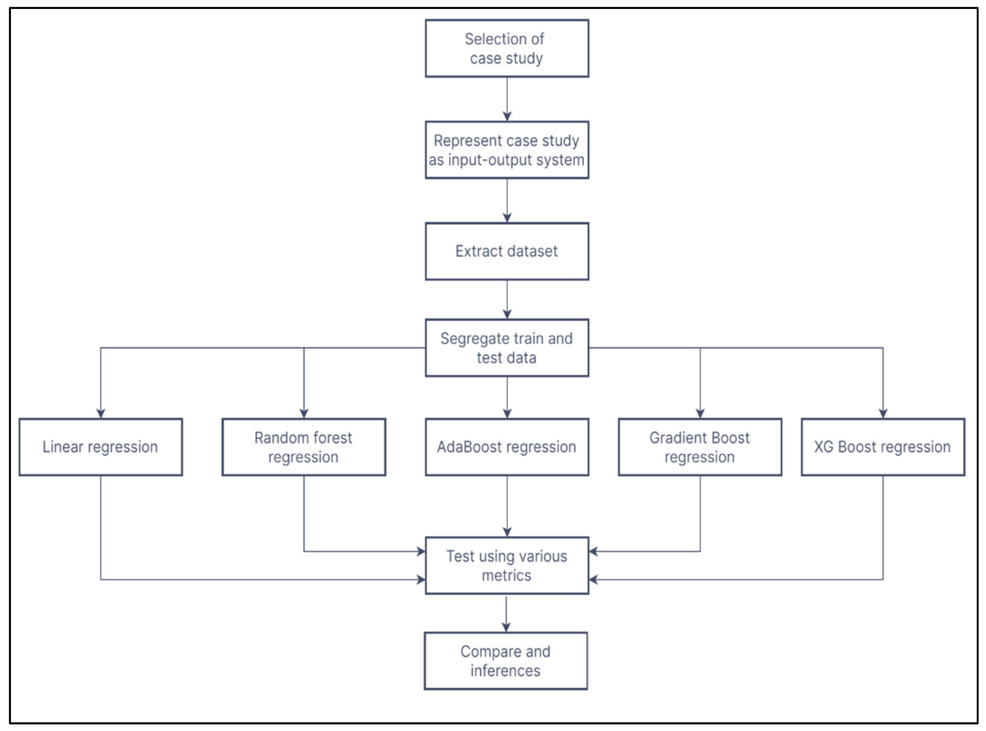
The methodology followed in this research is shown in the flowchart in Figure 1. Initially, suitable case studies from the literature are selected. After understanding the intricacies of the case study, they are represented as an input-output system. An input-output system is a simple way to represent the cause-and-effect phenomenon in the 3D printing system. The user-controllable process parameters, i.e., the variables, are the independent parameters. They are the input part of the input-output system. The properties of the components fabricated are the outputs or the dependent variables. These dependent variables can be expressed as functions of the independent variables. The goal of the machine learning predictive models is to examine and develop this relationship between the independent and dependent variables. Once the predictive models are developed, they are tested by using various statistical metrics to determine their predictive power.
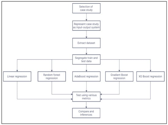
Figure 1.
Flowchart of the methodology.
2.1. Linear Regression
The linear regression method lies within the class of supervised machine learning. The method aids in estimating or explaining a given numerical value based on a group of data, for instance, estimating the cost of an asset based on the past pricing data for similar assets [28]. Linear regression uses the mathematical equation of the line to model a dataset:
Several data pairs are used to train the linear regression model through computing the position and gradient (slope) of a line which reduces the overall distance between all of the data points and the given line. That is, the -intercept and slope are calculated for a line which best estimates the observation in the data [29].
The key objective of linear regression is the construction of effective models for predicting the dependent attributes from a class of attribute variables. The method aims at identifying a positive correlation between two variables if the two variables move along together, and at identifying a negative correlation if an increase in one variable causes a decline in the other variable. The statistical equation of linear regression is:
where and are the dependent and independent variables, respectively [30]. In a multiple linear regression with estimators available, the equation will be:
where is the -intercept, , , , … are the coefficient of the dependent variable, is the dependent variable, and , , , … are the independent variables.
2.2. Random Forest Regression
Random forest regression is a supervised machine learning technique which is constructed from a decision tree algorithm. It uses the concept of ensemble learning, an approach of adding several classifiers to improve the model performance and solve complex problems. The method contains several decision trees on different subsets of a given data set and takes the mean to enhance the estimated accuracy of that data set [31]. Rather than depending on a single decision tree, random forest regression uses the estimation from every tree based on majority prediction votes and then estimates the final output. The precision of a random forest depends on the number of trees. The higher the number of trees in the forest, the higher the accuracy of the outcome. The greater the number of trees in the forest also helps in preventing the challenges of overfitting the data set [32].
The algorithm of random forest regression contains several decision trees. The resulting forest from a random forest regression algorithm is trained by bootstrap aggregating or bagging. Bagging enhances the accuracy of machine learning. The algorithm then determines the final result based on the decision tree predictions. A random forest regression algorithm generally performs well on several problems even in non-linear relationship features [33]. However, drawbacks with the method are that there is no interpretability, and overfitting can occur easily.
2.3. AdaBoost Regression
AdaBoost is a boosting ensemble machine learning approach. AdaBoost regression is a machine learning technique that starts by fitting a regressor on a data set, after which it fits extra copies of the regressor on the same data set, but in cases in which the weights of instances are adjusted as per the error of the prevailing estimation. As a result, the regressors that follow focus more on challenging cases. AdaBoost integrates the estimations for short single-level decision trees known as decision stumps, even though other algorithms may be used as well. Decision stump algorithms are utilized as the AdaBoost algorithm tries to utilize several weak models and rectify their estimators by combining additional weak models [34]. When training the AdaBoost regression algorithm, it starts with a single decision tree, then finds the examples in the training data set which were not properly classified and introduces additional weight to the examples. Other trees are then trained on the same data, however, there are now weighted errors due to misclassification. The procedure continues until all the desired number of trees are added. In case there is a false estimation, it is identified and then assigned further to the following base classifier that has a low weight. This process is repeated until the algorithm properly classifies the output.
2.4. Gradient Boosting Regression
Gradient boosting is a machine learning method that is based on the ensemble approach known as boosting. The method sequentially adds several weak learners to create a strong learner. This is an analytical method that is used to explore the association between two or more variables and generate prediction models. The output from the model is used in identifying significant factors that affect the dependent variables and the kind of association that exists between each of the factors and the dependent variable. It is important to note that GBR is limited to estimating numeric output, as such, the dependent variable must be numeric [35].
The GBR method is mainly used in regression approaches. The models used for prediction in gradient boost regression are often represented as decision trees. The gradient boosting regression is developed in a stage-wise manner. Decision trees, in gradient boosting, are the weak learners. Gradient boosting regression involves the following steps: (1) Construction of a base tree having one node. This acts as the starting guess for each sample. (2) Construct a tree based on errors from the preceding tree. (3) Tree scaling by the learning rate. The learning rate establishes the contribution of the tree in the estimation. (4) Join the resulting tree with each of the previous trees to estimate the outcome and redo step 2 until an optimum number of trees is realized or when the resulting tree does not affect the fit.
2.5. XGBoost Regression
XGBoost is a robust technique for creating supervised regression models. XGBoost regression is a method that provides an effective and efficient implementation of the gradient boosting models. The technique can be directly used for regression predictive modeling. The method is developed to be both highly effective and computationally efficient (for instance, fast to execute. XGBoost is mostly used for two key reasons. The first is model performance and the second is speed of execution. The technique dominates tabular and structured data sets on both regression and classification problems of predictive modeling [36]. The XGBoost comprises the base learners and objective function. The objective function has a regularization term and loss function. Through the objective function, we learn about the difference between the predicted values and the actual values, that is, the degree of deviation of the model output from the actual values. The approach uses ensemble learning that encompasses training and adding base learners (individual models) to obtain one prediction. XGBoost anticipates containing the base learners that are uniformly bad at the remainder so that once the estimations are added, the bad predictions can cancel out and the good predictions can add up to make the last good estimation.
3. Case Study 1
3.1. Problem Description
The importance of an accurate prediction of tensile strength of 3D printed parts cannot be overstated. Owing to the intricate nature of components fabricated and the cost involved in 3D printing, it is essential to develop accurate prediction models to predict the tensile strength of these parts. The data considered in this case study is from Bialete et al. [37]. They fabricated PLA filaments using 3D printing technology. Fused deposition modeling was used by them. A typical schematic of FDM is shown in Figure 2. The fabricated parts were in the shape of ASTM D638 dog bone-shape tensile test specimens. The tensile strength of the specimens was measured by a universal testing machine (10kN, Shimadzu AGS-X model). Three variable process parameters, namely, extrusion temperature, layer height, and shell thickness were considered. All the parameters were considered as equally spaced three-level parameters, i.e., extrusion temperature was varied between 190–220 °C, and layer height was considered between 0.2–0.4 mm. Shell thickness was between 0.4–1.2 mm for the experiments. A full factorial design (FFD) consisting of 27 experiments by varying the three process parameters was carried out. Apart from these three variable parameters, the constant parameters considered were a linear infill pattern with 100% infill percentage, raster angle of 45°, printing speed of 60 mm/s, and building direction along the x-axis. Bialete et al. [37] used an ANOVA-based approach to determine the effect of the process parameters. However, no prediction model or optimization was carried out by Bialete et al. [37].
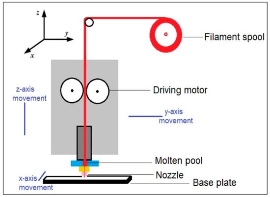
Figure 2.
Schematic of fused deposition modeling process.
3.2. Results and Discussion
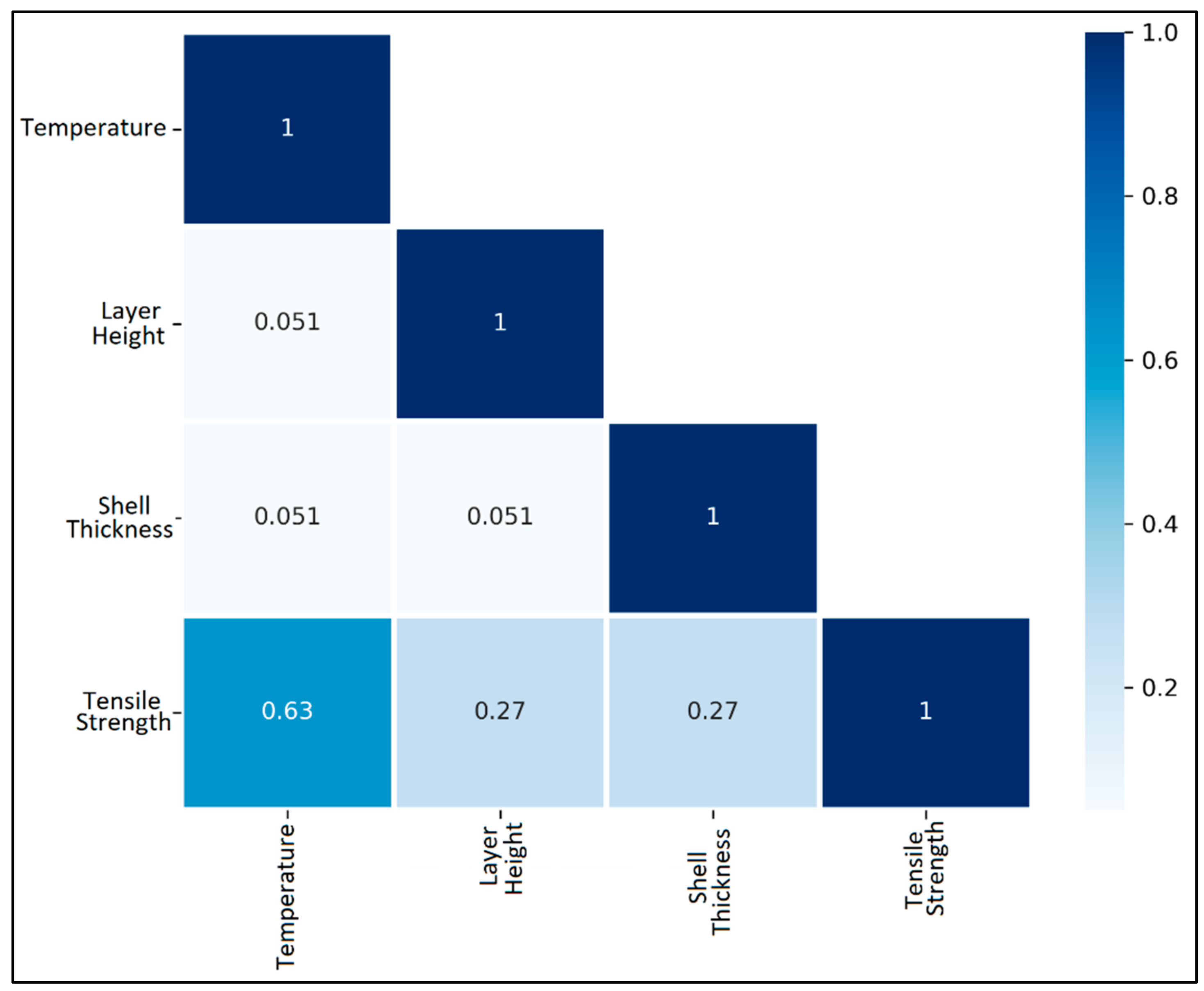
The correlation of the process parameters with the tensile strength is assessed via a Pearson correlation heatmap in Figure 3. The Pearson correlation is calculated for each pair of the process parameters, as well as for each process parameter and response pair, by using the following formula:
where is the correlation coefficient, and are the variables among whom correlation is to be found. and are the mean values of the variables in the sample.

Figure 3.
Pearson correlation heatmap for process parameters and tensile strength for case study 1.
It is observed that tensile strength shares a moderately strong positive correlation with temperature. However, both layer height and shell thickness maintain a weak positive correlation with tensile strength. Further, the lack of multicollinearity among the process parameters in the data is seen, which is an advantage in developing prediction models.
The five different ML algorithms selected in this work are then deployed to develop prediction models of the tensile strength of the 3D printed parts. It should be noted that all ML algorithms have a lot of hyperparameters which must be tuned to develop more accurate models. The optimized hyperparameters are calculated using a pilot study on the data. For the hyperparameter tuning, minimization of the MSE of the testing data set was considered the objective. The hyperparameters used for each algorithm are mentioned in Table 1.

Table 1.
Hyperparameter values used in this study.
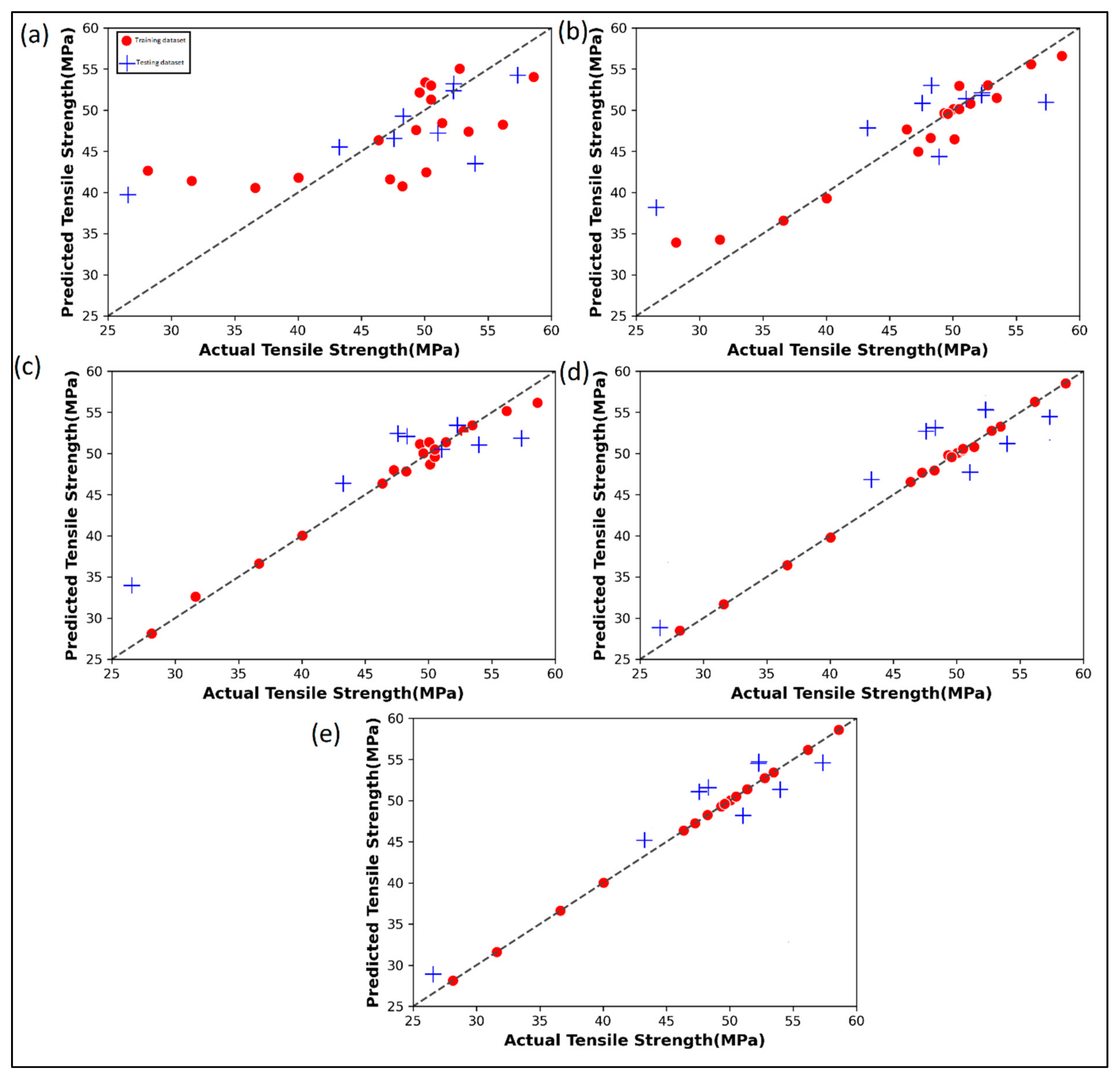
Figure 4 shows the prediction performance of the five ML algorithms for both training and testing data. The actual tensile strength versus the linear regression predicted values in Figure 4a show that there are significant deviations, even for the training set. It is seen that for the linear regression algorithm that the developed model is more prone to overprediction at lower tensile strength values but is prone to underprediction at higher tensile strength values. In Figure 4b, the random forest regression performs a little better than the linear regression on training data. However, the performance on testing is quite poor as before. In the case of AdaBoost regression (Figure 4c), there is a remarkable improvement in the fitting characteristics of the training data over random forest regression and linear regression. However, the performance of testing data remains poor. Gradient boost regression (Figure 4d) and the XGBoost regression (Figure 4e) can fit the training data in an ideal manner, wherein all the predicted training data points are seen hugging the diagonal identity line. The testing data performance of XGBoost is found to be a little better than the gradient boost algorithm. Moreover, in both these two algorithms, the testing data are found to have an equal affinity for underprediction as well as overprediction. This indicates that the models are not biased and they are equally likely to overpredict or underpredict a new data point. The predicted values by each ML algorithm for the given case study are shown in Table A1.
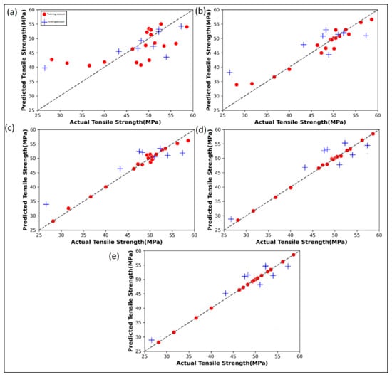
Figure 4.
Actual versus predicted tensile strength by various ML algorithms: (a) Linear regression; (b) Random Forest regression; (c) AdaBoost regression; (d) Gradient boost regression; (e) XGBoost regression for case study 1.
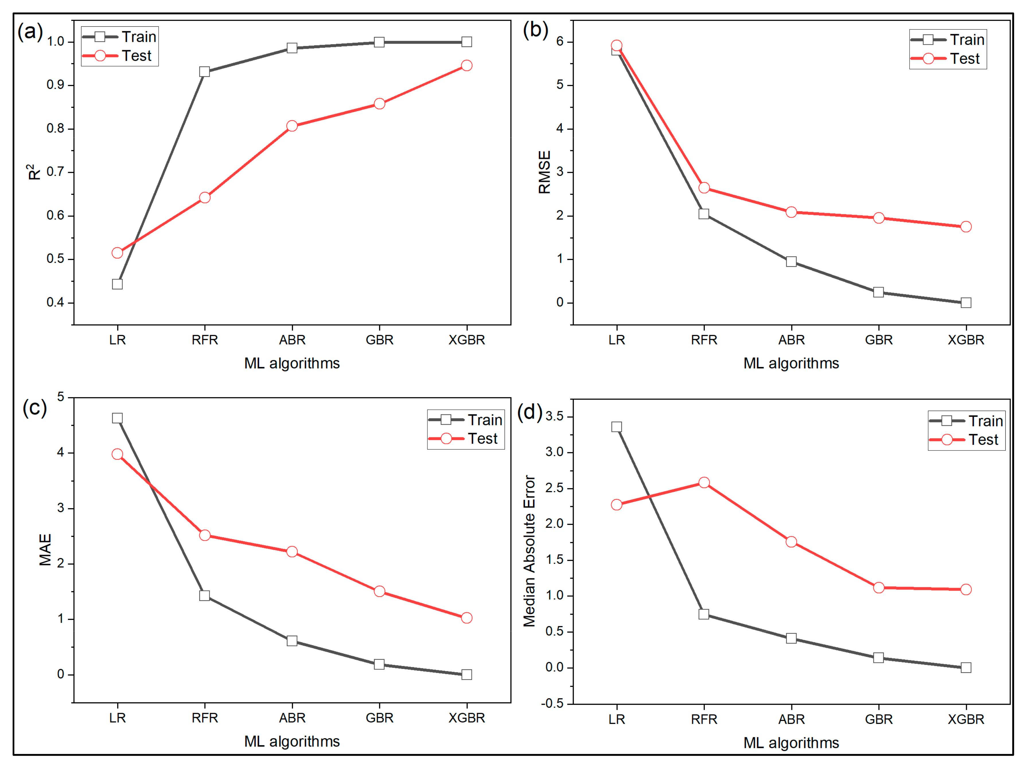
The tensile strength prediction models developed by the five different ML algorithms are tested using four different statistical metrics. Kalita et al. [38] pointed out that every statistical metric depicts only a certain trait of the prediction model and thus, multiple metrics should be consulted before choosing or rejecting a model. Figure 5a shows the performance of the ML algorithms using metric. The linear regression model can explain only 44% of the variance in the training data but luckily fares a little better on the testing data. On the other hand, random forest, AdaBoost, gradient boost and XGBoost record approximately 93%, 98.5%, 99.9%, and 100%, respectively on training data. On testing data, the random forest, AdaBoost, gradient boost, and XGBoost falls and are 64%, 80%, 85%, and 94.6%, respectively. XG boost model shows remarkable improvement over the other four algorithms in terms of RMSE, MAE and median absolute error as well as shown in Figure 5b–d, respectively. XGBoost is about 70% better than linear regression in terms of RMSE, 74% and 52% better in terms of MAE and median absolute error, respectively. Overall, from the analysis, it can be concluded from the first case study that in terms of prediction performance, the models can be ranked from inferiority to superiority as linear regression < random forest < AdaBoost < gradient boost < XGBoost.
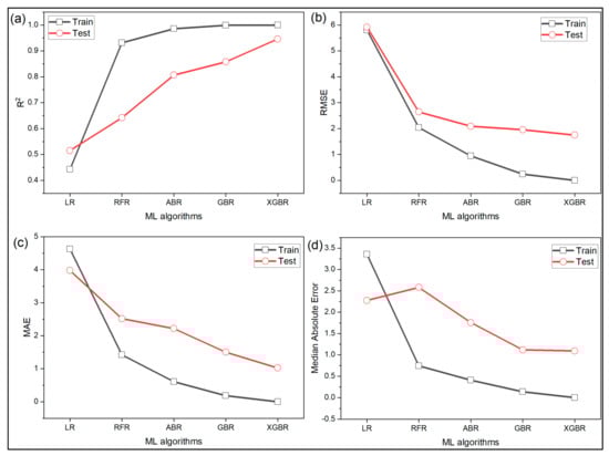
Figure 5.
Performance of various ML algorithms measured using (a) ; (b) root mean squared error; (c) mean absolute error; (d) median absolute error for case study 1.
4. Case Study 2
4.1. Problem Description
The data for the second case study was considered from Rai et al. [7]. Rai et al. [7] considered four process parameters, namely, layer thickness and build orientation with respect to XY, XZ, and YZ planes. The layer thickness varied between 0.0889–0.1016 mm whereas the build orientation with respect to XY, XZ, and YZ planes was considered to be between 0° to 90° with increments of 45°. A Box–Behnken experimental design (BBD) was used. The BBD ensures that instead of the 81 experiments needed for FFD, only 27 experiments were enough to have the same statistical relevance of the experiment design. The specimens in dog bone-shape tensile test specimens were fabricated in ZPrinter450 3D printer using ZP150 powder as the material. Using a universal testing machine, the tensile strengths of the specimens were measured. The CAD models and 3D printed specimens are shown in Figure A1. Regression analysis was used by Rai et al. [7] to develop a predictive model for the tensile strength as given below:
where represents layer thickness, , and indicate the angle in plane, angle in plane, and angle in plane, respectively.
The developed model by Rai et al. [7] suffers from two main deficiencies—first, it has not been tested against any independent test data. Secondly, it is assumed in their regression analysis that all the terms of the model are statistically significant, which may have potentially led to bloating of the metric. Further, no additional statistical metric such as adjusted , MSE, MAE, etc., is mentioned, which impaired the wholistic assessment of the developed prediction model.
4.2. Results and Discussion
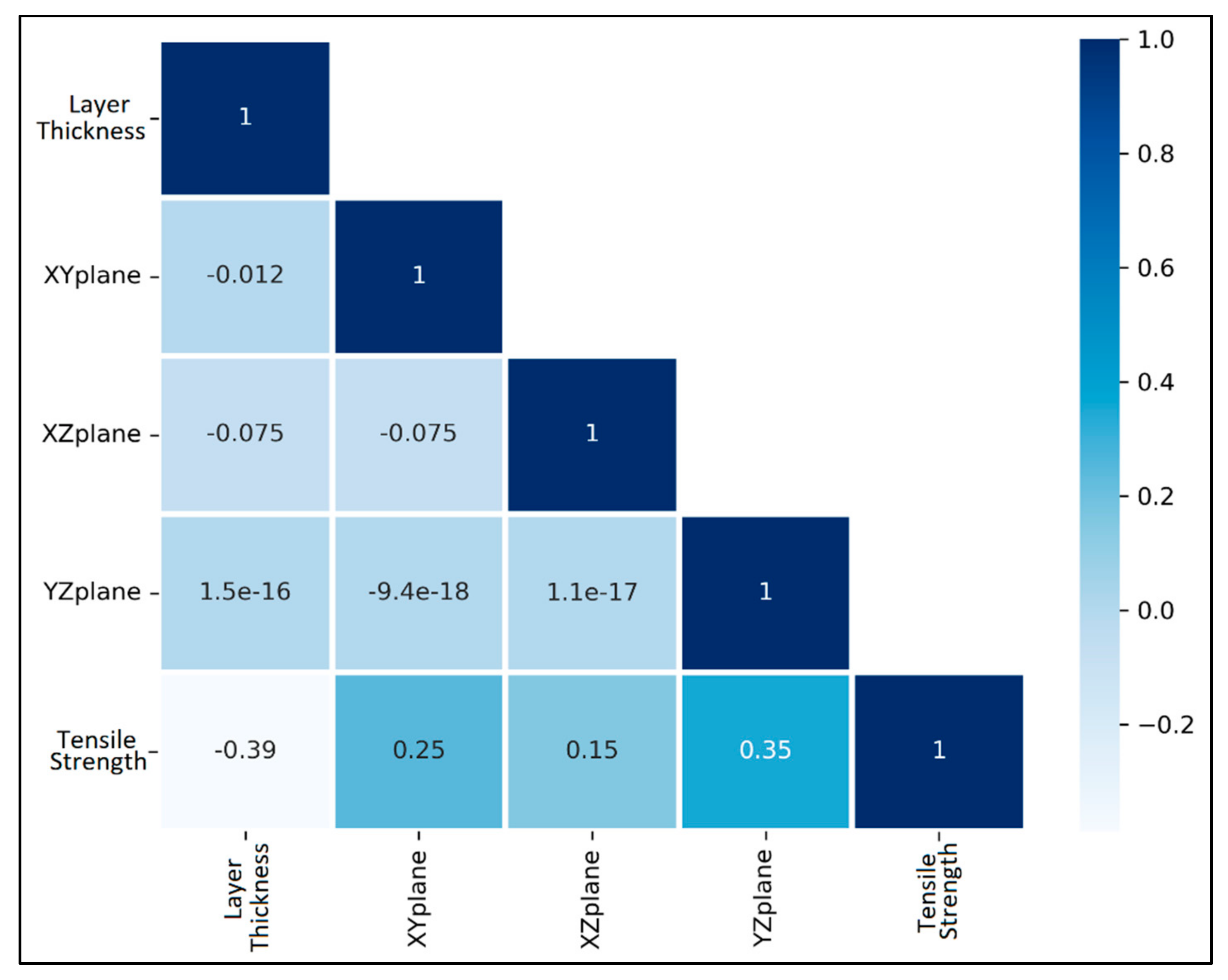
The Pearson correlation heatmap of the layer thickness, angle in XY plane, angle in XZ plane, and angle in YZ plane against tensile strength is plotted in Figure 6. The Pearson correlations are calculated by using Equation (4). The tensile strength has a relatively low negative correlation with the layer thickness, i.e., as the layer thickness increases, the tensile strength of the component is likely to go down. The angle in the XY plane, angle in the XZ plane, and angle in the YZ plane has a low positive correlation with the tensile strength. There is also no multicollinearity in the data as all the independent variables possess no correlation amongst themselves.
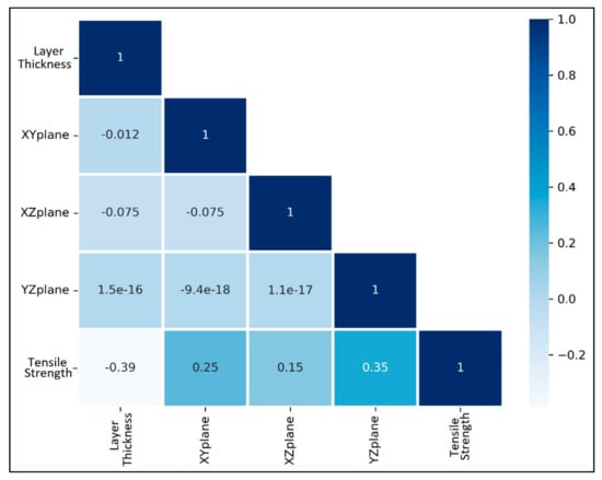
Figure 6.
Pearson correlation heatmap for process parameters and tensile strength for case study 2.
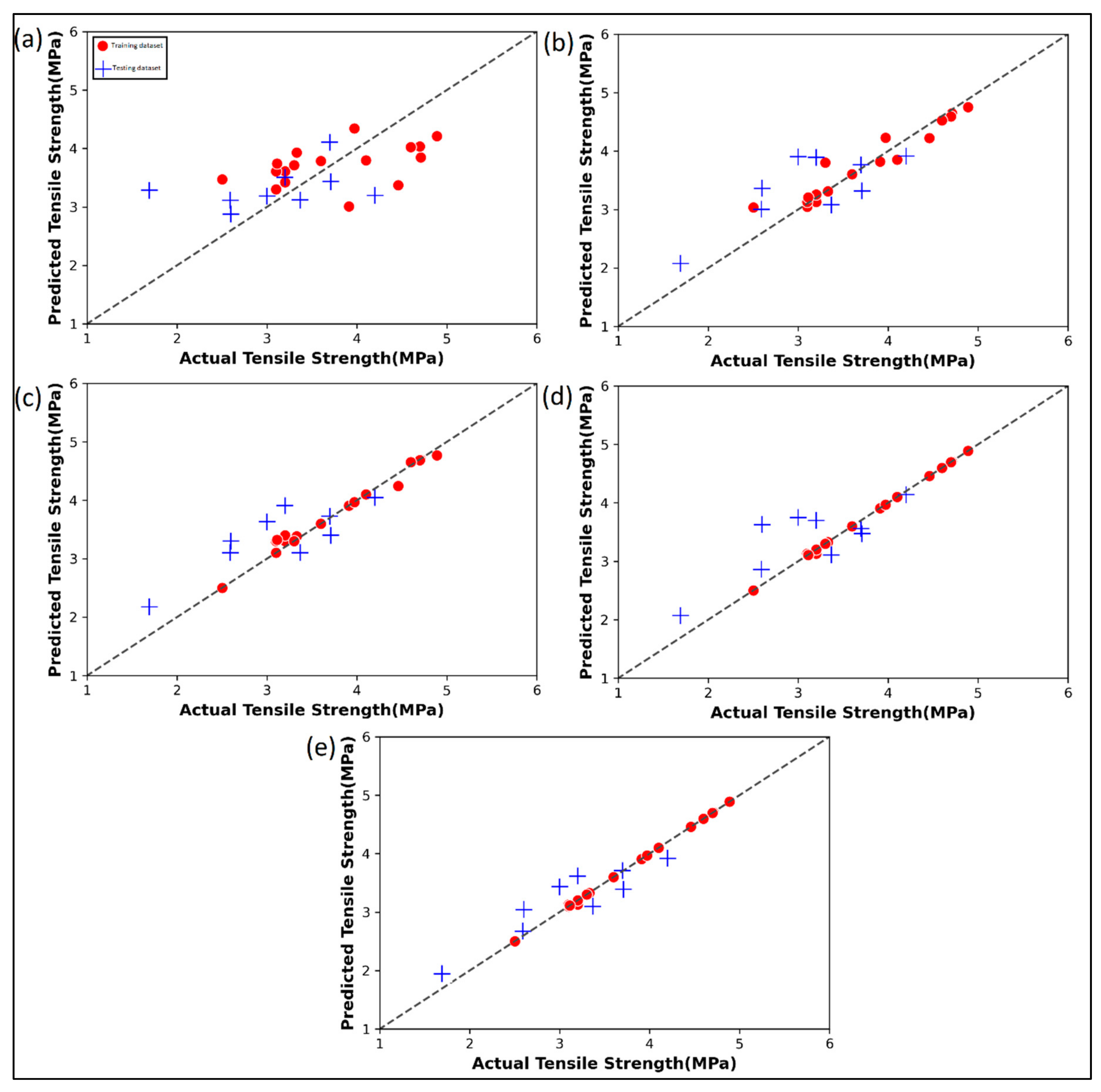
Figure 7 shows the actual versus the predicted tensile strength of the 3D printed parts. The red dots indicate the performance of the ML algorithms on training data whereas the blue ones indicate the performance on testing data. In Figure 7a, a cluster pattern is observed in the mid-section of the tensile strength range. Additionally, the linear regression model in Figure 7a is seen to have larger underpredictions. The random forest regression model (Figure 7b) has a relatively better performance, but still contains significant errors in the testing data. The AdaBoost (Figure 7c) has similar performances to the random forest regression. In the gradient boost regression model (Figure 7d), the training data is exactly mapped as indicated by the points hugging the diagonal identity line. The XGBoost model (Figure 7e) has significant improvement over all the other four ML models. Table A2 shows the predicted values by each ML algorithm for the given case study.
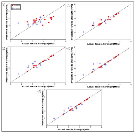
Figure 7.
Actual versus predicted tensile strength by various ML algorithms: (a) Linear regression; (b) Random Forest regression; (c) AdaBoost regression; (d) Gradient boost regression; (e) XG Boost regression for case study 2.
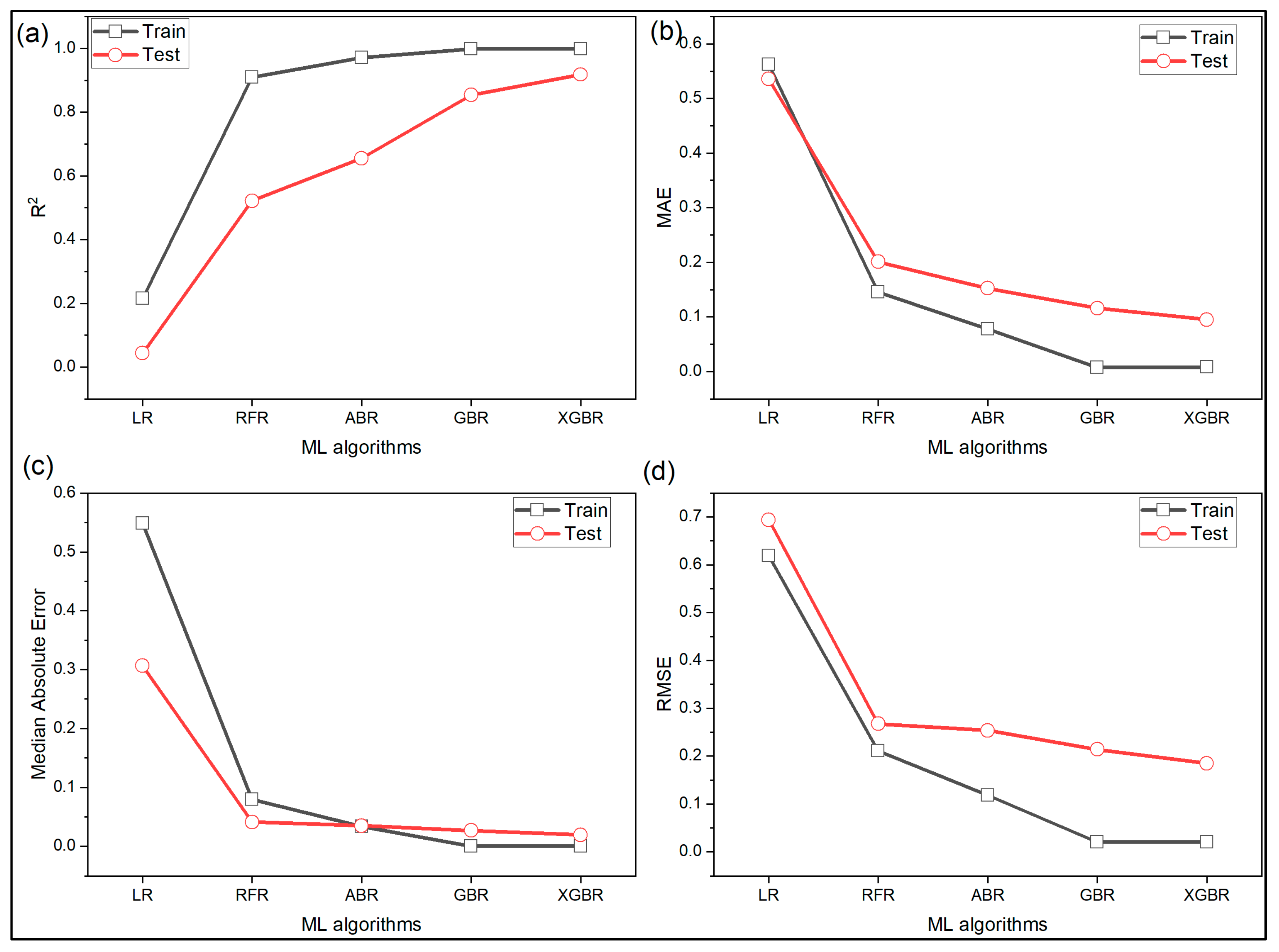
The accuracy of the models is measured using various statistical metrics and shown in Figure 8. The linear regression model performed the worst. As seen from Figure 8a, the linear regression, random forest, AdaBoost, gradient boost and XGBoost record 21%, 90%, 97%, 99.9%, and 99.9%, respectively on for training data but there is a significant drop in for testing data. It was 4%, 52%, 65%, 85%, and 91.8% for linear regression, random forest, AdaBoost, gradient boost, and XGBoost, respectively. Figure 8b shows the performance of the ML models based on MAE. It is seen that the random forest, AdaBoost, gradient boost, and XGBoost are 74%, 86%, 99%, and 99% better than linear regression on training and 63%, 72%, 78%, and 82% better on testing data. Similar inferences can be drawn based on median absolute error and RMSE from Figure 8c,d, respectively.
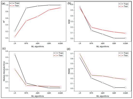
Figure 8.
Performance of various ML algorithms measured using (a) ; (b) mean absolute error; (c) median absolute error; (d) root mean squared error for case study 2.
Based on all the four metrics, the ML algorithm-based models can be ranked as linear regression < random forest < AdaBoost < gradient boost < XGBoost.
It should be noted that the prime objective of any process planning and optimization task is to establish empirical relationships between some control variables (such as table feed, layer thickness, nozzle diameter, material temperature, etc.) and evaluation responses (such as tensile strength of the printed object, surface roughness, printing time, cost, etc.). In most cases, the challenge is to quantify the variability or uncertainty of these control variables. As such, the possibility distribution-based method provides a better result [39], as it factors in the uncertainty associated with the data and process in the analysis. Such analysis makes use of fuzzy numbers to develop an association between the process parameters and responses. However, these methods are generally more computationally intensive as compared to crisp methods. The methodology followed in this study is data-driven and is unaffected by the underlying physics of the processes. Thus, the same approach can be readily used for any other material as well. However, it should be noted that the methods are expected to perform much better when trained on well-designed uniformly distributed datasets [40].
5. Conclusions
Efficient and accurate prediction of the mechanical properties of 3D printed parts is of great significance for improving the productivity of the process and reducing downtime. In this paper, two case studies were considered wherein various process parameters of the 3D printing were treated as the inputs to an ML-based prediction system, which then predicted the tensile strength of the part. In the first case study, the extrusion temperature, layer height, and shell thickness were treated as the inputs while in the second case study, the layer thickness and build orientation with respect to XY, XZ, and YZ planes were the input parameters. Based on the elaborate analysis, the following conclusions can be drawn:
- The overall in case study 1 for both training and testing data are 48%, 79%, 90%, 93%, and 97% for linear regression, random forest, AdaBoost, gradient boost and XGBoost regression, respectively. For case study 2, the respective are 13%, 72%, 81%, 93%, and 96%.
- The testing data RMSE for case study 1 for the random forest, AdaBoost, gradient boost and XGBoost regression has 55%, 65%, 67%, and 70% improvement over the linear regression. Similarly, for case study 2, the respective improvement in testing data RMSE are 61%, 63%, 69% and 73%.
- The MAE for testing has 37%, 44%, 62%, and 74% improvement in case study 1 and 63%, 72%, 78%, and 82% improvement in case study 2 for the random forest, AdaBoost, gradient boost and XGBoost regression as compared to linear regression.
- The five tested ML algorithms can be ranked based on superiority as XGBoost > gradient boost > AdaBoost > random forest > linear regression.
One of the limitations of this study is that the comparison is not exhaustive. There are several other ML algorithms such as support vector regression, multi-layer perceptron regression, hist gradient boosting regression, etc., which are not considered in this study. Another limitation of the study is the search for optimum hyperparameters without the use of any global optimization algorithms. In future, this study will be extended to include more ML algorithms and other case studies. It is expected that these outcomes will be helpful to practitioners looking to implement ML technology to improve existing machining or manufacturing processes.
Author Contributions
Conceptualization, M.E. and M.M.; Data curation, M.J. and J.P.; Formal analysis, M.J. and J.P.; Investigation, M.J. and J.P.; Methodology, M.J., M.E., M.M. and J.P.; Software, M.E., M.M. and J.P.; Supervision, M.E.; Visualization, M.J. and J.P.; Writing—original draft, M.J. and M.E.; Writing—review and editing, M.M. All authors have read and agreed to the published version of the manuscript.
Funding
This work was supported by the project SP2022/60 Applied Research in the Area of Machines and Process Control supported by the Ministry of Education, Youth and Sports, Czech Republic.
Institutional Review Board Statement
Not applicable.
Informed Consent Statement
Not applicable.
Data Availability Statement
The data presented in this study are available through email upon request to the corresponding author.
Conflicts of Interest
The authors declare no conflict of interest.
Appendix A
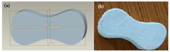
Figure A1.
(a) CAD model of test specimen; (b) 3D printed specimen [7].
Figure A1.
(a) CAD model of test specimen; (b) 3D printed specimen [7].
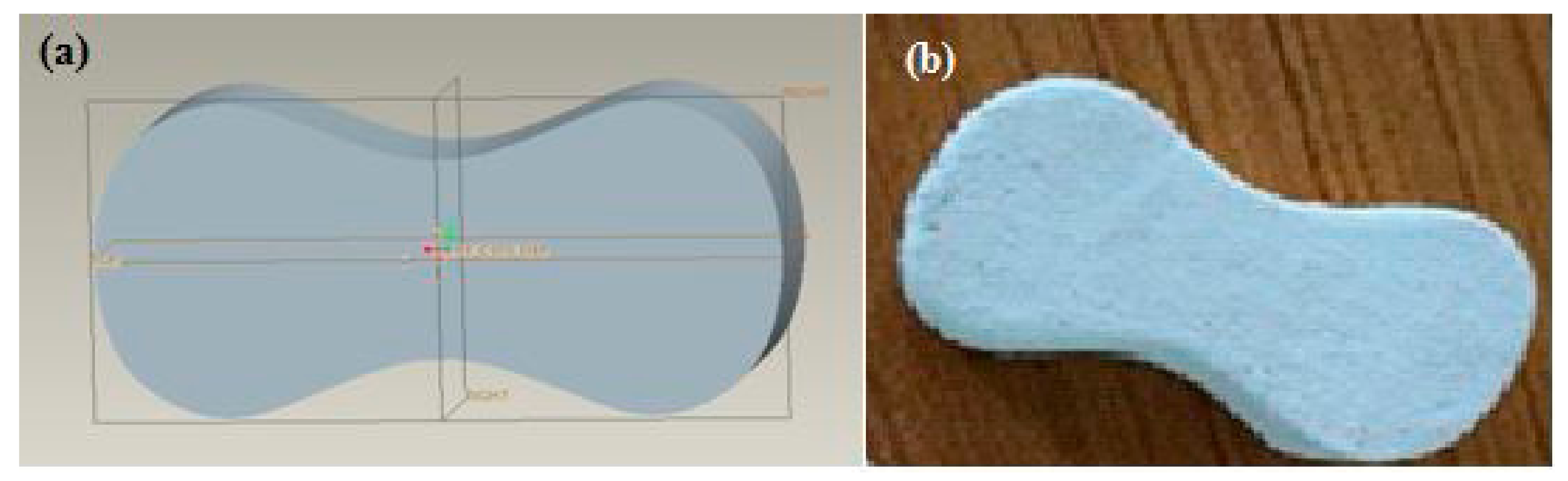
Table A1.
Predicted tensile strength values by different ML algorithms for case study 1.
Table A1.
Predicted tensile strength values by different ML algorithms for case study 1.
| Dataset Type | Process Parameters | Tensile Strength (MPa) | |||||||
|---|---|---|---|---|---|---|---|---|---|
| Extrusion Temperature (°C) | Layer Height (mm) | Shell Thickness (mm) | Expt. [37] | LR | RFR | ABR | GBR | XGBR | |
| Train | 205 | 0.30 | 0.80 | 53.4510 | 47.4039 | 51.5042 | 53.4510 | 53.2953 | 53.4503 |
| Train | 205 | 0.40 | 0.40 | 49.3090 | 47.6049 | 49.6641 | 51.1500 | 49.7884 | 49.3099 |
| Train | 190 | 0.20 | 0.80 | 36.6240 | 40.5744 | 36.5884 | 36.6240 | 36.4268 | 36.6197 |
| Train | 190 | 0.30 | 0.80 | 47.2660 | 41.6123 | 44.9661 | 47.9770 | 47.6849 | 47.2696 |
| Train | 190 | 0.30 | 1.20 | 50.1100 | 42.4492 | 46.4725 | 48.6880 | 49.9946 | 50.1075 |
| Train | 190 | 0.20 | 1.20 | 31.5910 | 41.4113 | 34.2525 | 32.5976 | 31.6920 | 31.5949 |
| Train | 205 | 0.40 | 0.80 | 51.3720 | 48.4418 | 50.7908 | 51.3720 | 50.8032 | 51.3701 |
| Train | 220 | 0.30 | 1.20 | 58.6040 | 54.0324 | 56.6093 | 56.1700 | 58.5133 | 58.6012 |
| Train | 190 | 0.30 | 0.40 | 48.2420 | 40.7754 | 46.6527 | 47.8348 | 47.9529 | 48.2422 |
| Train | 220 | 0.40 | 1.20 | 52.7540 | 55.0703 | 53.0392 | 52.7540 | 52.7619 | 52.7541 |
| Train | 220 | 0.40 | 0.40 | 50.0400 | 53.3965 | 50.1411 | 51.3720 | 50.0583 | 50.0410 |
| Train | 220 | 0.20 | 0.40 | 50.5010 | 51.3207 | 50.1393 | 49.5990 | 50.4251 | 50.4996 |
| Train | 220 | 0.40 | 1.20 | 52.7540 | 55.0703 | 53.0392 | 52.7540 | 52.7619 | 52.7541 |
| Train | 220 | 0.20 | 1.20 | 50.4910 | 52.9945 | 52.9521 | 50.4910 | 50.5557 | 50.4909 |
| Train | 190 | 0.40 | 0.80 | 28.1300 | 42.6502 | 33.9174 | 28.1300 | 28.4666 | 28.1331 |
| Train | 205 | 0.20 | 0.80 | 46.3540 | 46.3660 | 47.6776 | 46.3540 | 46.5454 | 46.3553 |
| Train | 205 | 0.30 | 1.20 | 56.1700 | 48.2408 | 55.6098 | 55.1687 | 56.3085 | 56.1707 |
| Train | 220 | 0.20 | 0.80 | 49.5990 | 52.1576 | 49.5674 | 50.0450 | 49.5552 | 49.6001 |
| Train | 190 | 0.40 | 0.40 | 40.0240 | 41.8133 | 39.2817 | 40.0240 | 39.7959 | 40.0217 |
| Test | 205 | 0.20 | 0.40 | 43.2540 | 45.5291 | 47.8368 | 46.3540 | 46.8259 | 46.7304 |
| Test | 220 | 0.40 | 0.80 | 57.3320 | 54.2334 | 50.9692 | 51.8327 | 50.7039 | 50.6326 |
| Test | 190 | 0.40 | 1.20 | 53.9810 | 43.4871 | 35.8518 | 28.1300 | 30.8207 | 32.7860 |
| Test | 220 | 0.30 | 0.40 | 52.2740 | 52.3586 | 51.8048 | 53.4510 | 56.0195 | 55.4502 |
| Test | 190 | 0.20 | 0.40 | 26.5880 | 39.7375 | 38.1897 | 36.6240 | 36.7842 | 37.1562 |
| Test | 205 | 0.30 | 0.40 | 47.5860 | 46.5670 | 50.8308 | 52.4115 | 52.7035 | 52.4950 |
| Test | 205 | 0.40 | 1.20 | 48.3070 | 49.2787 | 53.0190 | 52.0650 | 53.1198 | 53.0042 |
| Test | 220 | 0.30 | 0.80 | 52.2990 | 53.1955 | 52.1130 | 53.4510 | 55.9680 | 55.6377 |
| Test | 205 | 0.20 | 1.20 | 51.0320 | 47.2029 | 51.3811 | 50.4910 | 44.4346 | 45.9100 |
Table A2.
Predicted tensile strength values by different ML algorithms for case study 2.
Table A2.
Predicted tensile strength values by different ML algorithms for case study 2.
| Dataset Type | Process Parameters | Tensile Strength (MPa) | ||||||||
|---|---|---|---|---|---|---|---|---|---|---|
| Layer Thickness (mm) | XY Plane | XZ Plane | YZ Plane | Expt. [7] | LR | RFR | ABR | GBR | XGBR | |
| Train | 0.10 | 45 | 45 | 45 | 3.0900 | 3.6122 | 3.1293 | 3.3033 | 3.1300 | 3.1305 |
| Train | 0.09 | 90 | 45 | 45 | 3.3300 | 3.9320 | 3.3143 | 3.3825 | 3.3300 | 3.3303 |
| Train | 0.10 | 45 | 90 | 0 | 4.4600 | 3.3743 | 4.2226 | 4.2440 | 4.4600 | 4.4583 |
| Train | 0.10 | 45 | 0 | 90 | 4.7100 | 3.8501 | 4.6465 | 4.7000 | 4.7100 | 4.7087 |
| Train | 0.10 | 90 | 45 | 45 | 3.1000 | 3.2992 | 3.0484 | 3.1000 | 3.1000 | 3.0985 |
| Train | 0.10 | 90 | 45 | 90 | 4.7000 | 4.0376 | 4.5910 | 4.6850 | 4.7000 | 4.7003 |
| Train | 0.10 | 0 | 90 | 45 | 3.6000 | 3.7879 | 3.6075 | 3.6000 | 3.6000 | 3.6000 |
| Train | 0.10 | 45 | 0 | 0 | 3.9100 | 3.0110 | 3.8223 | 3.9100 | 3.9100 | 3.9102 |
| Train | 0.10 | 45 | 45 | 45 | 3.2000 | 3.6122 | 3.1293 | 3.3033 | 3.1300 | 3.1305 |
| Train | 0.10 | 90 | 90 | 45 | 4.1000 | 3.7997 | 3.8552 | 4.1000 | 4.1000 | 4.1003 |
| Train | 0.09 | 45 | 45 | 90 | 3.9700 | 4.3456 | 4.2307 | 3.9700 | 3.9700 | 3.9700 |
| Train | 0.10 | 45 | 45 | 45 | 3.1000 | 3.6122 | 3.1293 | 3.3033 | 3.1300 | 3.1305 |
| Train | 0.10 | 0 | 0 | 45 | 3.2000 | 3.4247 | 3.2588 | 3.4000 | 3.2000 | 3.2001 |
| Train | 0.09 | 45 | 0 | 45 | 3.1100 | 3.7445 | 3.2050 | 3.3220 | 3.1100 | 3.1112 |
| Train | 0.10 | 45 | 90 | 45 | 2.5000 | 3.4749 | 3.0374 | 2.5000 | 2.5000 | 2.5004 |
| Train | 0.10 | 0 | 45 | 90 | 4.6000 | 4.0258 | 4.5284 | 4.6525 | 4.6000 | 4.6004 |
| Train | 0.10 | 45 | 45 | 90 | 3.3000 | 3.7128 | 3.8047 | 3.3000 | 3.3000 | 3.3006 |
| Train | 0.10 | 45 | 90 | 90 | 4.8900 | 4.2134 | 4.7532 | 4.7667 | 4.8900 | 4.8890 |
| Test | 0.10 | 45 | 0 | 45 | 2.5900 | 3.1116 | 3.0023 | 3.1000 | 2.8604 | 2.6710 |
| Test | 0.10 | 90 | 0 | 45 | 3.3700 | 3.1175 | 3.0832 | 3.1000 | 3.1074 | 3.0980 |
| Test | 0.09 | 45 | 90 | 45 | 3.7000 | 4.1077 | 3.7634 | 3.7250 | 3.5584 | 3.7084 |
| Test | 0.10 | 90 | 0 | 45 | 3.7100 | 3.4364 | 3.3201 | 3.4033 | 3.4747 | 3.3897 |
| Test | 0.10 | 0 | 45 | 45 | 1.6900 | 3.2874 | 2.9973 | 3.1000 | 2.8458 | 2.6984 |
| Test | 0.10 | 0 | 45 | 0 | 3.0000 | 3.1868 | 3.9028 | 3.6300 | 4.0749 | 3.9192 |
| Test | 0.09 | 45 | 45 | 0 | 3.2000 | 3.5066 | 3.8916 | 3.9100 | 4.0244 | 3.9188 |
| Test | 0.10 | 45 | 45 | 0 | 2.6000 | 2.8737 | 3.6656 | 3.3000 | 3.9540 | 3.6375 |
| Test | 0.10 | 90 | 45 | 0 | 4.2000 | 3.1985 | 3.9133 | 4.0475 | 4.1429 | 3.9192 |
References
- Goh, G.D.; Sing, S.L.; Yeong, W.Y. A review on machine learning in 3D printing: Applications, potential, and challenges. Artif. Intell. Rev. 2021, 54, 63–94. [Google Scholar] [CrossRef]
- Murr, L.E. Metallurgy principles applied to powder bed fusion 3D printing/additive manufacturing of personalized and optimized metal and alloy biomedical implants: An overview. J. Mater. Res. Technol. 2020, 9, 1087–1103. [Google Scholar] [CrossRef]
- Leal, R.; Barreiros, F.M.; Alves, L.; Romeiro, F.; Vasco, J.C.; Santos, M.; Marto, C. Additive manufacturing tooling for the automotive industry. Int. J. Adv. Manuf. Technol. 2017, 92, 1671–1676. [Google Scholar] [CrossRef]
- Kong, L.; Ambrosi, A.; Nasir, M.Z.M.; Guan, J.; Pumera, M. Self-Propelled 3D-Printed “Aircraft Carrier” of Light-Powered Smart Micromachines for Large-Volume Nitroaromatic Explosives Removal. Adv. Funct. Mater. 2019, 29, 1903872. [Google Scholar] [CrossRef]
- Nasiri, S.; Khosravani, M.R. Machine learning in predicting mechanical behavior of additively manufactured parts. J. Mater. Res. Technol. 2021, 14, 1137–1153. [Google Scholar] [CrossRef]
- Kalita, K.; Haldar, S.; Chakraborty, S. A Comprehensive Review on High-Fidelity and Metamodel-Based Optimization of Composite Laminates. Arch. Comput. Methods Eng. 2022, 1–36. [Google Scholar] [CrossRef]
- Rai, H.V.; Modi, Y.K.; Pare, A. Process parameter optimization for tensile strength of 3D printed parts using response surface methodology. IOP Conf. Ser. Mater. Sci. Eng. 2018, 377, 012027. [Google Scholar] [CrossRef] [Green Version]
- Srinivasan, R.; Pridhar, T.; Ramprasath, L.S.; Charan, N.S.; Ruban, W. Prediction of tensile strength in FDM printed ABS parts using response surface methodology (RSM). Mater. Today Proc. 2020, 27, 1827–1832. [Google Scholar] [CrossRef]
- Azli, A.A.; Muhammad, N.; Albakri, M.M.A.; Ghazali, M.F.; Rahim, S.Z.A.; Victor, S.A. Printing parameter optimization of biodegradable PLA stent strut thickness by using response surface methodology (RSM). IOP Conf. Ser. Mater. Sci. Eng. 2020, 864, 012154. [Google Scholar] [CrossRef]
- Deshwal, S.; Kumar, A.; Chhabra, D. Exercising hybrid statistical tools GA-RSM, GA-ANN and GA-ANFIS to optimize FDM process parameters for tensile strength improvement. CIRP J. Manuf. Sci. Technol. 2020, 31, 189–199. [Google Scholar] [CrossRef]
- Saad, M.S.; Nor, A.M.; Baharudin, M.E.; Zakaria, M.Z.; Aiman, A.F. Optimization of surface roughness in FDM 3D printer using response surface methodology, particle swarm optimization, and symbiotic organism search algorithms. Int. J. Adv. Manuf. Technol. 2019, 105, 5121–5137. [Google Scholar] [CrossRef]
- Vates, U.K.; Kanu, N.J.; Gupta, E.; Singh, G.K.; Daniel, N.A.; Sharma, B.P. Optimization of FDM 3D printing process parameters on ABS based bone hammer using RSM technique. IOP Conf. Ser. Mater. Sci. Eng. 2021, 1206, 012001. [Google Scholar] [CrossRef]
- Yao, X.; Moon, S.K.; Bi, G. A hybrid machine learning approach for additive manufacturing design feature recommendation. Rapid Prototyp. J. 2017, 23, 983–997. [Google Scholar] [CrossRef]
- DeCost, B.L.; Jain, H.; Rollett, A.D.; Holm, E.A. Computer vision and machine learning for autonomous characterization of am powder feedstocks. JOM 2017, 69, 456–465. [Google Scholar] [CrossRef] [Green Version]
- Jiang, J.; Hu, G.; Li, X.; Xu, X.; Zheng, P.; Stringer, J. Analysis and prediction of printable bridge length in fused deposition modelling based on back propagation neural network. Virtual Phys. Prototyp. 2019, 14, 253–266. [Google Scholar] [CrossRef]
- Shen, X.; Yao, J.; Wang, Y.; Yang, J. Density prediction of selective laser sintering parts based on artificial neural network. In Proceedings of the International Symposium on Neural Networks, Dalian, China, 19–21 August 2004. [Google Scholar] [CrossRef]
- Ye, D.; Fuh, J.Y.H.; Zhang, Y.; Hong, G.S.; Zhu, K. In situ monitoring of selective laser melting using plume and spatter signatures by deep belief networks. ISA Trans. 2018, 81, 96–104. [Google Scholar] [CrossRef]
- Gu, G.X.; Chen, C.-T.; Richmond, D.J.; Buehler, M.J. Bioinspired hierarchical composite design using machine learning: Simulation, additive manufacturing, and experiment. Mater. Horiz. 2018, 5, 939–945. [Google Scholar] [CrossRef] [Green Version]
- Lu, Z.L.; Li, D.C.; Lu, B.H.; Zhang, A.F.; Zhu, G.X.; Pi, G. The prediction of the building precision in the Laser Engineered Net Shaping process using advanced networks. Opt. Lasers Eng. 2010, 48, 519–525. [Google Scholar] [CrossRef]
- Kabaldin, Y.G.; Shatagin, D.A.; Anosov, M.S.; Kolchin, P.V.; Kiselev, A.V. Diagnostics of 3D Printing on a CNC Machine by Machine Learning. Russ. Eng. Res. 2021, 41, 320–324. [Google Scholar] [CrossRef]
- Mahmood, M.A.; Visan, A.I.; Ristoscu, C.; Mihailescu, I.N. Artificial neural network algorithms for 3D printing. Materials 2020, 14, 163. [Google Scholar] [CrossRef]
- Nguyen, P.D.; Nguyen, T.Q.; Tao, Q.B.; Vogel, F.; Nguyen-Xuan, H. A data-driven machine learning approach for the 3D printing process optimisation. Virtual Phys. Prototyp. 2022, 1–19. [Google Scholar] [CrossRef]
- Zhang, H.; Moon, S.K.; Ngo, T.H. Hybrid machine learning method to determine the optimal operating process window in aerosol jet 3D printing. ACS Appl. Mater. Interfaces 2019, 11, 17994–18003. [Google Scholar] [CrossRef]
- Menon, A.; Póczos, B.; Feinberg, A.W.; Washburn, N.R. Optimization of silicone 3D printing with hierarchical machine learning. 3D Print. Addit. Manuf. 2019, 6, 181–189. [Google Scholar] [CrossRef]
- Ağbulut, Ü.; Gürel, A.E.; Biçen, Y. Prediction of daily global solar radiation using different machine learning algorithms: Evaluation and comparison. Renew. Sustain. Energy Rev. 2021, 135, 110114. [Google Scholar] [CrossRef]
- Markovics, D.; Mayer, M.J. Comparison of machine learning methods for photovoltaic power forecasting based on numerical weather prediction. Renew. Sustain. Energy Rev. 2022, 161, 112364. [Google Scholar] [CrossRef]
- Nourani, M.; Alali, N.; Samadianfard, S.; Band, S.S.; Chau, K.-W.; Shu, C.-M. Comparison of machine learning techniques for predicting porosity of chalk. J. Pet. Sci. Eng. 2022, 209, 109853. [Google Scholar] [CrossRef]
- Harishkumar, K.S.; Yogesh, K.M.; Gad, I. Forecasting air pollution particulate matter (PM2.5) using machine learning regression models. Procedia Comput. Sci. 2020, 171, 2057–2066. [Google Scholar] [CrossRef]
- Bhattacharya, S.; Kalita, K.; Čep, R.; Chakraborty, S. A Comparative Analysis on Prediction Performance of Regression Models during Machining of Composite Materials. Materials 2021, 14, 6689. [Google Scholar] [CrossRef] [PubMed]
- Yao, W.; Li, L. A new regression model: Modal linear regression. Scand. J. Stat. 2014, 41, 656–671. [Google Scholar] [CrossRef] [Green Version]
- Gupta, K.K.; Kalita, K.; Ghadai, R.K.; Ramachandran, M.; Gao, X.-Z. Machine Learning-Based Predictive Modelling of Biodiesel Production—A Comparative Perspective. Energies 2021, 14, 1122. [Google Scholar] [CrossRef]
- Jain, P.; Choudhury, A.; Dutta, P.; Kalita, K.; Barsocchi, P. Random Forest Regression-Based Machine Learning Model for Accurate Estimation of Fluid Flow in Curved Pipes. Processes 2021, 9, 2095. [Google Scholar]
- Kalita, K.; Shinde, D.S.; Ghadai, R.K. Machine Learning-Based Predictive Modelling of Dry Electric Discharge Machining Process. In Data-Driven Optimization of Manufacturing Processes; IGI Global: Hershey, PA, USA, 2021; pp. 151–164. [Google Scholar] [CrossRef]
- Cao, Y.; Miao, Q.-G.; Liu, J.-C.; Gao, L. Advance and prospects of AdaBoost algorithm. Acta Autom. Sin. 2013, 39, 745–758. [Google Scholar] [CrossRef]
- Zhang, Y.; Haghani, A. A gradient boosting method to improve travel time prediction. Transp. Res. Part C Emerg. Technol. 2015, 58, 308–324. [Google Scholar] [CrossRef]
- Shanmugasundar, G.; Vanitha, M.; Čep, R.; Kumar, V.; Kalita, K.; Ramachandran, M. A Comparative Study of Linear, Random Forest and AdaBoost Regressions for Modeling Non-Traditional Machining. Processes 2021, 9, 2015. [Google Scholar] [CrossRef]
- Bialete, E.R.; Manuel, M.C.E.; Alcance, R.M.E.; Canlas, J.P.A.; Chico, T.J.B.; Sanqui, J.P.; Cruz, J.C.D.; Verdadero, M.S. Characterization of the Tensile Strength of FDM-Printed Parts Made from Polylactic Acid Filament using 33 Full-Factorial Design of Experiment. In Proceedings of the 2020 IEEE 12th International Conference on Humanoid, Nanotechnology, Information Technology, Communication and Control, Environment, and Management (HNICEM), Manila, Philippines, 3–7 December 2020. [Google Scholar] [CrossRef]
- Kalita, K.; Dey, P.; Haldar, S. Search for accurate RSM metamodels for structural engineering. J. Reinf. Plast. Compos. 2019, 38, 995–1013. [Google Scholar] [CrossRef]
- Chowdhury, M.A.K.; Ullah, A.M.M.; Teti, R. Optimizing 3D Printed Metallic Object’s Postprocessing: A Case of Gamma-TiAl Alloys. Materials 2021, 14, 1246. [Google Scholar] [CrossRef]
- Kalita, K.; Chakraborty, S.; Madhu, S.; Ramachandran, M.; Gao, X.-Z. Performance analysis of radial basis function metamodels for predictive modelling of laminated composites. Materials 2021, 14, 3306. [Google Scholar] [CrossRef]

Publisher’s Note: MDPI stays neutral with regard to jurisdictional claims in published maps and institutional affiliations. |
© 2022 by the authors. Licensee MDPI, Basel, Switzerland. This article is an open access article distributed under the terms and conditions of the Creative Commons Attribution (CC BY) license (https://creativecommons.org/licenses/by/4.0/).