Surrogate-Assisted Multi-Objective Optimization of a Liquid Oxygen Vacuum Subcooling System Based on Ejector and Liquid Ring Pump

Abstract

As an important combustion aid for aerospace vehicles, subcooled liquid oxygen of high density can be used to increase loading capacity of a spacecraft. Providing a large amount of cryogenic propellant in a short time with a strict energy consumption limitation is a challenge in the design of the fuel filling system. The authors proposed a vacuumed subcooling system combined with an ejector and liquid ring pump to vacuum a liquid oxygen tank and obtain subcooled liquid oxygen. After the liquid oxygen tank is vacuumed to an intermediate pressure by the ejector, it is further vacuumed to 10 kPa using the liquid ring pump. The infinitesimal method was used to simulate the thermodynamic processes involved. Taking the ejector working fluid mass flow rate, jet pressure, intermediate pressure, initial tank liquid level, and liquid ring pump speed as optimizing variables, optimization was conducted to determine the optimal vacuuming time, remaining liquid level in the tank, pumping speed difference, and nitrogen consumption. The sample set was generated by the optimal Latin sampling algorithm. The surrogate assisted Non-dominated Sorting Genetic Algorithm (NSGA-III) multi-objective algorithm was used to construct a system optimization framework. The non-dominated solutions were added to the sample set to improve the generalization ability of the Gaussian Process Regression (GPR) in the Pareto front. A convergent Pareto solution set was obtained after multiple iterations. The influence of different optimization variables on each optimization objective was analyzed using the Pearson correlation coefficient method. The optimization results show that the trade-off scheme can obtain the subcooled liquid oxygen at 10 kPa and 73 K with a remaining liquid level of 74.84% in a total vacuum time of 19.93 h. The efficiency of the liquid oxygen vacuum subcooling system can be improved significantly.

1. Introduction

In aerospace cryogenic engineering, the use of subcooled liquid oxygen as a combustion aid can significantly increase the loading capacity of the rocket owing to its high density. The Soviet Union “Soyuz” rocket used a 70 K subcooled liquid oxygen filling system [1,2,3], and the “Энергия” rocket used a 57 K liquid oxygen subcooling system [4]. In a combined saturated liquid nitrogen and vacuumed subcooling liquid-nitrogen system, the liquid-nitrogen bath is evacuated to obtain subcooled liquid nitrogen. Then, liquid oxygen is subcooled by heat exchange with the subcooled liquid nitrogen. The NASA Glenn Center obtained 66.67 K subcooled liquid oxygen using this method [5,6]. Different subcooling methods have been proposed, and they have advantages and disadvantages in terms of safety and engineering difficulty. When a nitrogen ejector is used to vacuum the tank containing liquid oxygen, the vacuuming speed is high, but the consumption of high-pressure nitrogen is considerable. Moreover, accurate control of the temperature fluctuations is required if appropriate levels of subcooled liquid oxygen are to be obtained from heat exchange with subcooled liquid nitrogen. The “Falcon 9” rocket once carried liquid helium to cool liquid oxygen, but the subcooling was too difficult to control, causing the liquid oxygen freezing and the rocket explosion [7]. Thus, a number of cryogenic propellant filling systems with low energy consumption and high energy efficiency are needed at launch sites worldwide. In order to investigate the subcooling cryogenic liquid by vacuuming, Zuo [8] designed and built a visualized cryogenic fluid evaporation test bench to measure the interfacial temperature profile of evaporating liquid oxygen in atmospheric pressure. The modified KTG model has a good agreement with experiment data. The present authors proposed a subcooling system combined with an ejector and liquid ring pump to vacuum a liquid oxygen tank and obtain subcooled liquid oxygen. After the liquid oxygen tank is vacuumed to an intermediate pressure by the ejector, it is further vacuumed to 10 kPa by The liquid ring pump. The subcooled liquid oxygen at 73 K is to be yielded in the subcooling system. Here, the optimal operation conditions for the ejector and liquid ring pump will be determined, and a highly efficient optimization method is proposed in this study.

In the field of thermodynamic process optimization, the optimization frameworks, such as GA (Genetic Algorithm), are used to connect the steady-state thermodynamics solver [9]. Khan [10] investigated a multi-optimization of a dual-mixed refrigerant natural gas liquefaction process based on NSGA-II (Non-dominated Sorting Genetic Algorithm II, NSGA-II), where having the specific compression power and the heat exchanger area as objectives results in savings of 36% and 15% respectively. Song [11] optimized a nitrogen expansion LNG process with carbon dioxide expansion precooling with NSGA-II for the objective of specific energy consumption and liquefaction rate; the result shows an increase of 5.19% (0.77–0.81) of liquefaction rate and a decrease of 10.1% of energy consumption. Mofid [12], using GA and MOPSO (multi-objective particle swarm optimization) to optimize a nitrogen expansion LNG process, takes the energy consumption and the liquefaction rate as objectives separately, and the result shows that MOPSO obtained better Pareto fronts in comparison of GA.

For most multi-objective optimization problems, the objectives are conflicting, and the improvement of one objective may lead to the degradation of the other objectives. It is impossible to optimize multiple objectives simultaneously, and only coordinated trade-offs and compromises can be made among the objectives to make all objective functions as optimal as possible. The optimal solution could not maximize all objective functions under a given constraint. Instead, a set of Pareto optimal solutions could be obtained.

A multi-objective optimization problem (MOP) can be expressed as follows:

$$\underset{\mathit{x}\in \mathcal{D}}{\min } y=f\left(x\right)=\left[f_1\left(x\right),\dots ,f_{\mathrm{j}}\left(x\right)\right]$$

$$\mathrm{s}.\mathrm{t}. g_{\mathrm{i}}\left(x\right)\le 0, I=1, 2, \dots , p$$

(1)

$$\mathcal{D}=\left[x^{\mathrm{lb}},x^{\mathrm{ub}}\right],$$

where the space of global solutions $\mathcal{D}=$ [$x^{\mathrm{lb}},x^{\mathrm{ub}}]$ represents the lower bound and upper bound of $x$, objective functions $y=f$, inequality constraints $g$, and $j$ is the number of objectives. $f\left(x\right)$ as a high-precision simulation function is expensive to calculate in order to accelerate the optimization process, therefore, it is efficient to use a data-driven surrogate-assisted optimization framework based on high-precision simulation samples [13].

So far, there are not many theoretical studies on operation conditions optimization for a cryogenic liquids subcooling system by vacuuming. This study proposed a simple prediction method for a liquid oxygen subcooling system on the basis of the quasi-steady state assumption in a micro time step. The heat and mass balances in the liquid oxygen subcooling system were simulated using an infinitesimal method. The thermodynamic model was verified by a liquid nitrogen vacuumed subcooling system with a maximum pressure deviation of 10.17% and a maximum liquid level deviation of 7.02%. A four-objective optimization algorithm based on NSGA-III and a Gaussian process regression optimized by a Bayesian optimization algorithm were used as the surrogate model to accelerate the optimization calculation. The adopted optimization algorithm efficiently obtains the four-objective Pareto frontier. If the vacuum ejector is operated at a multi-objective trade-off optimal conditions, i.e., a working fluid mass flow rate of 1 kg/s and a pressure of 5 Mpa, an intermediate pressure of 16.09 kPa, if the pump speed of liquid ring pump is 12.96 m³/min, 74.84% of the liquid oxygen remains at subcooled state in 19.93 h and the consumption of high pressure nitrogen is 2267.3 standard cubic meters (Sm³), it can meet the engineering limitation. The present study provides a reference for the multi-objective optimization of similar cryogenic liquid subcooling systems.

2. Methodology

This study aims to design a subcooling system combined with an ejector and liquid ring pump to vacuum a liquid oxygen tank and obtain subcooled liquid oxygen at 73 K. The volume of the liquid oxygen tank is assumed to be 60 m³. In order to yield the largest amount of subcooling liquid oxygen with the smallest energy consumption while in the shortest total vacuuming time, optimal operation parameters need to be determined based on this test system. Energy consumption contains the maximum available nitrogen storage and maximum available power. A previous investigation demonstrated that the high pumping speed of the ejector and the stable pumping speed of the liquid ring pump can optimize the vacuuming process. Therefore, the combined vacuum system with an ejector and liquid ring pump was adopted. A diagram of the proposed system is shown in Figure 1.

The liquid oxygen vacuum process is shown in Figure 1. At the beginning of the vacuuming process, the liquid oxygen stored in the tank is vacuumed by the ejector when valve SV4 is turned off and other valves are opened. The liquid oxygen is vacuumed to an intermediate pressure $p_s$, then valves SV2 and SV3 are closed and SV4 is opened. The vacuum system shifts to the liquid ring pump mode. The liquid oxygen tank is vacuumed with the liquid ring pump until the tank reaches the target pressure of 10 kPa to obtain subcooled liquid oxygen at 73 K. A heat exchanger is used to superheat the vacuumed cryogenic oxygen vapor before entering the liquid ring pump. To optimize the performance of the combined vacuum system, it is necessary to determine the key parameters of the system (nitrogen flow rate and jet pressure of the ejector, intermediate pressure $p_s$, initial tank liquid level, and liquid ring pump speed) and the total working time, nitrogen consumption, remaining liquid level, and pumping speed difference of the ejector and liquid ring pump.

2.1. Heat and Mass Balance of the Vacuumed Subcooling Process

In a micro time step of the vacuuming process, it can be regarded as being in a quasi-equilibrium state, and the mass conservation of the vacuum process can be expressed as:

$$\delta {\dot{m}}_{\mathrm{s}}+m_{\mathrm{r}}=m_{init}$$

(2)

$$\delta {\dot{m}}_{\mathrm{s}}=q_i\delta t,$$

(3)

where $m_{\mathrm{init}}$ (in kg) is the initial liquid oxygen mass at the beginning of the vacuuming process, and $\delta {\dot{m}}_{\mathrm{s}}$ (in kg) determined by Equation (3) is the mass of the liquid oxygen vacuumed from the initial pressure (p₁) to p₂ in the time step ($\delta t$ = 0.1 s). $q_i$ (in kg/s) represents the effective vacuuming mass flow rate. The remaining liquid oxygen mass (in kg) in the tank at the end of the time step, $m_{\mathrm{r}}$, can be determined by Equation (2).

The effective pumping speed is calculated by:

$$q_i=\frac{q_{\mathrm{e}}{U}_{\mathrm{t}}}{U_{\mathrm{t}}+q_{\mathrm{e}}},$$

(4)

where $q_i$ is the vacuum speed (or the effective vacuuming mass flow rate) in kg/s. $q_{\mathrm{e}}$ is the pump speed of the ejector and $q_{\mathrm{p}}$ is the pump speed of the liquid ring pump, and $U_{\mathrm{t}}$ is the flow conductance of the system.

Here, $q_{\mathrm{e}}$ can be determined by:

$$q_{\mathrm{e}}=\mu \delta {\dot{m}}_{{\mathrm{N}}_2}/\delta t,$$

(5)

where μ is the average ejection ratio of the pressure interval in the time step, $\mu =\delta {\dot{m}}_{\mathrm{s}}/\delta {\dot{m}}_{{\mathrm{N}}_2}$, and $\delta {\dot{m}}_{{\mathrm{N}}_2}$ is the mass of nitrogen entering the ejector in the micro time step. The performance of the ejector can be calculated based on an isobaric mixing model [14]. According to the working fluid pressure ($p_{\mathrm{e}}$) of the ejector, nitrogen mass ($m_{{\mathrm{N}}_2}$), efficiency of the nozzle, efficiency of the mixing chamber, efficiency of the expansion section (${\eta }_{\mathrm{N}}$, ${\eta }_{\mathrm{m}}$, ${\eta }_{\mathrm{d}}$), and other parameters, the vacuumed fluid pressure $p_s$ (i.e., the liquid oxygen storage tank pressure) can be calculated.

For the liquid ring pump, the effective pump speed under different storage tank pressures ($q_{\mathrm{p}}$) can be determined. Therefore, the mass of the vacuumed gas can be calculated as follows:

$$\delta {\dot{m}}_{\mathrm{s}}=\delta {\dot{V}}_{\mathrm{ex}}{\overline{\rho }}_{\mathrm{g}}=q_{\mathrm{p}}\delta t_{\mathrm{p}},$$

(6)

where ${\overline{\rho }}_{\mathrm{g}}$ is the average density of the gas in the time step.

The vacuumed gas in the micro time step ($\delta {\dot{m}}_{\mathrm{s}}$) is vaporized by two mechanisms.

$$\delta {\dot{m}}_{\mathrm{s}}=\delta {\dot{m}}_{\mathrm{flash}}+\delta {\dot{m}}_{\mathrm{heatleak}},$$

(7)

where $\delta {\dot{m}}_{\mathrm{flash}}$ is the mass of liquid oxygen flashing caused by the pressure drop, and $\delta {\dot{m}}_{\mathrm{heatleak}}$ is the mass of liquid oxygen evaporation caused by heat leakage, and it can be determined by the daily evaporation rate of the liquid oxygen tank (0.5%).

$$\delta {\dot{m}}_{\mathrm{heatleak}}=\frac{0.005m_{\mathrm{init}}\delta t}{24\times 3600}.$$

(8)

The energy conservation equation for the vacuumed subcooling process can be expressed as:

$$\delta {\dot{m}}_{\mathrm{flash}}{\gamma }_2=m_{\mathrm{r}}\Delta h_{\mathrm{l}1-2}+\delta {\dot{m}}_{\mathrm{O}2}\Delta h_{\mathrm{g}1-2}+C_{\mathrm{s}}{m}_{\mathrm{W}}\Delta T ,$$

(9)

where ${\gamma }_2$ is the latent heat of liquid oxygen at pressure p₂; $\Delta h_{\mathrm{l}1-2}$ is the liquid-phase enthalpy difference in the time step; $\delta {\dot{m}}_{\mathrm{O}2}$ is the mass difference of the gas-phase in the time step; $\Delta h_{\mathrm{g}1-2}$ is the gas-phase enthalpy difference in the time step; $C_{\mathrm{s}}$ is the tank wall heat capacity; ${\dot{m}}_{\mathrm{W}}$ is the mass of the tank inner wall, and $\Delta T$ is the tank wall temperature difference in the time step.

The total vacuuming time is:

$$t_{\mathrm{T}}=t_{\mathrm{e}}+t_{\mathrm{p}}.$$

(10)

The working time of the liquid ring pump ($t_{\mathrm{p}}$) is $n_{\mathrm{p}}\delta t_{\mathrm{p}}$, and $n_{\mathrm{e}}$ and $n_{\mathrm{p}}$ are the iteration times of the ejector and liquid ring pump program, respectively. Here, $\delta t_{\mathrm{e}}$ and $\delta t_{\mathrm{p}}$ are the micro time steps of the operation of the ejector and liquid ring pump, respectively. The total nitrogen consumption $V_{\mathrm{tc}}$ (Sm³) can be determined by $\left(\int \delta {\dot{m}}_{{\mathrm{N}}_2}\delta t_{\mathrm{e}}\right)/{\rho }_{\mathrm{std}}$ and the nitrogen density under standard conditions (${\rho }_{\mathrm{std}}$) is 1.2504 kg/m³.

The tank pressure and remaining liquid oxygen mass at different time steps can be determined by solving the mass and energy conservation equations. Then, the volume of the remaining liquid oxygen in the storage tank ($V_{\mathrm{r},\mathrm{LO}2}$) can be calculated using the equation V_rLO2 = m_r/ρ_i, where ${\rho }_i$ is the liquid oxygen density at the corresponding pressure and is determined by the thermal properties database of Refprop. Thus, the final remaining tank level ($leve{l}_{\mathrm{r}}$) can be calculated by $V_{\mathrm{r},\mathrm{LO}2}/V_{\tan \mathrm{k}}$.

To utilize the maximum vacuuming capacity of the ejector, the vacuum speed of the ejector should be as high as possible, although it gradually decays with decreasing of the tank pressure. Therefore, the differential pressure drop rate of the element ($\delta sp$) was chosen as a coefficient to assess the vacuuming process.

$$\delta sp=\frac{\delta p_{\mathrm{el}}}{\delta t_{\mathrm{e}}}-\frac{\delta p_{\mathrm{pf}}}{\delta t_{\mathrm{p}}},$$

(11)

where $\delta p_{\mathrm{el}}$ is the pressure drop at the last micro time step using the vacuuming ejector, and $\delta p_{\mathrm{pf}}$ is the pressure drop of the first micro time period employing the liquid ring pump. When $\delta sp$ is negative, the vacuuming scheme is unreasonable.

The aim of this study was to determine an optimal operating condition for a liquid oxygen vacuumed subcooling system. The limitations of the available conditions are listed in

Table 1. Limitations of engineering conditions.

Engineering Conditions	Limitation
Storage of N2 (Nm3)	2300
Available motor power (kW)	<110
Total vacuuming time (h)	<24
Volume of LO2 tank (m3)	60

.

2.2. Validation of the Simulation Method

A liquid nitrogen vacuumed subcooling test system was used for experimental validation. The schematic diagram and the test set of the vacuumed subcooling system are shown in Figure 2 and Figure 3. The tank pressure and the remaining liquid level were used as the verifying indicators. The above mentioned quasi-equilibrium model was used to simulate the vacuumed subcooling of liquid nitrogen. Due to the high thermodynamic similarity of nitrogen and oxygen, the validated model can be used for the simulation of the vacuumed subcooling of liquid oxygen.

Although only the liquid ring pump was verified, both the simulation models for ejector and liquid ring pump were given in the abovementioned model, and the vacuuming speed for different devices has been specified in Equation (4). The vacuuming performance of the ejector can be correctly predicted by the validated simulation model using the specification of the vacuuming speed of the ejector.

The test conditions were specified as follows. The liquid nitrogen storage tank was 60 m³. The diameter of the exhaust gas pipeline connecting the heat exchanger was 0.08 m, the pipe length was 20 m, and the pressure drop in the pipe was 2.44 kPa. The diameter of the nitrogen channel in the heat exchanger was 0.018 m, the total length of the pipeline was 84 m, and the pressure drop was 38.17 kPa. The liquid ring pump speed was 0.25 m³/s. Nitrogen was heated to 283 K in the heat exchanger. The simulation results and experimental data are shown in Figure 4.

As shown in Figure 4, the liquid nitrogen tank was vacuumed to a lower pressure, and the simulated tank liquid level deviated from the experimental results considerably. This may be because the liquid level fluctuates violently, but the simulation data cannot reflect the dynamic fluctuation of the liquid level, resulting in a maximum deviation of 7.02%. The simulation results for the tank pressure agreed well with the experimental data. When the vacuum time was approximately 10,000 s, the deviation of the simulated pressure was less than 10.17%. The pressure in the vacuumed tank can be measured more accurately than the liquid level. On the basis of the micro time discretization, the vacuumed tank pressure can also be simulated correctly. So, the simulated pressures matched the experimental data well. However, cryogenic liquid level measurement is very challenging, and there is an unclear phase interface in the tank due to the rapid evaporation of cryogenic liquid, and a relatively large uncertainty exists in the cryogenic liquid level measurement. On the other hand, the present simulation was based on the quasi-steady state assumption and the heat and mass transfer are ignored.

2.3. Surrogate Based Multi-Optimization

The optimization of the liquid oxygen vacuumed subcooling process can be formulated as follows:

$$\begin{array}{c}\underset{\mathit{x}\in \mathcal{D}}{\min }=f\left(x\right)=[f_1\left(x\right),f_2\left(x\right),f_3\left(x\right),f_4\left(x\right)]=[t_{\mathrm{T}},\left|V_{\mathrm{tc}}-2300\right|,-leve{l}_{\mathrm{r}},-\delta sp]\\ x=\left[m_{{\mathrm{N}}_2},p_{\mathrm{e}},p_{\mathrm{s}},s_{\mathrm{p}},leve{l}_{\mathrm{init}}\right]\\ \mathcal{D}=\left[x^{\mathrm{lb}},x^{\mathrm{ub}}\right].\end{array}$$

(12)

In the optimal operation of the vacuumed subcooling process, the remaining liquid oxygen level should achieve the maximum value in the shortest period. So, the optimization of $t_{\mathrm{T}}$ and $leve{l}_{\mathrm{r}}$ are in opposite directions. The difference between the consumed nitrogen volume ($V_{\mathrm{tc}}$) and the maximum nitrogen storage (2300 Sm³) is one of the optimizing objectives. $-\delta sp$ is another objective of the optimization. The lower and upper bounds are shown in

Table 2. Range of sampling variables.

Optimization Variables	Sampling Lower Bound	Sampling Upper Bound
$m_{{\mathrm{N}}_2}$ (kg/s)	0.1	1
$p_{\mathrm{e}}$ (MPa)	1	5
$p_{\mathrm{s}}$ (kPa)	10	90
$leve{l}_{\mathrm{init}}$ (%)	83	95
$s_{\mathrm{p}}$ (m3/min)	5	25

.

The simulation (infinitesimal solver) is a time consuming unsteady thermal dynamics solver, and it is necessary to call the solver repeatedly during the optimization process. Thus, a surrogate model was established to accelerate the optimization process. Thus, the multi-objective optimization problem can be reformed as:

$$\underset{\mathit{x}\in \mathcal{D}}{\min } y=f_{\mathrm{s}}\left(x\right),$$

(13)

where the surrogate model $f_{\mathrm{s}}\left(x\right)$ is a black box function based on a data-driven approach. Generally, the establishment of a surrogate model has four steps, ensuring the sampling boundary, sampling, selecting the surrogate model, and hyperparameter optimization.

First, the actual product parameters are used to obtain the sampling boundary. The optimization variables are shown in Equation (12). The sampling ranges of the optimization variables are listed in Table 2.

Then, the samples ($X={\left[x^{\left(1\right)}\dots x^{\left(i\right)}\right]}^T$) were generated by the optimal Latin hypercube sampling method [15]. Simulations were performed for each sample and then regression responses $y=f\left(x\right)$ were obtained as:

$$y=f\left(x\right)={\left[\begin{array}{c}{f}_1\left(x^{\left(1\right)}\right)\dots f_1\left(x^{\left(i\right)}\right)\\ f_2\left(x^{\left(1\right)}\right)\dots f_2\left(x^{\left(i\right)}\right)\\ f_3\left(x^{\left(1\right)}\right)\dots f_3\left(x^{\left(i\right)}\right)\\ f_4\left(x^{\left(1\right)}\right)\dots f_4\left(x^{\left(i\right)}\right)\end{array}\right]}^T.$$

(14)

Sample set D consists of optimization variables and a regression response. $D=\left[X,y\right]$. Based on the sample set $D$, linear regression [16], regression trees [17], support vector regression (SVR) [18], Gaussian process regression (GPR) [19], ensemble trees [20] and the fivefold cross validation were used to obtain the surrogate model performance, as shown in

Table 3. Comparison of the R-squared of surrogate models.

Regression Response	Linear Regression	Regression Trees	Support Vector Machine	Gaussian Process Regression	Ensemble Trees
$t_{\mathrm{T}}$ (s)	0.83	0.68	0.94	0.95	0.64
$leve{l}_{\mathrm{r}}$ (%)	1.0	1.0	0.99	1	0.77
$\delta sp$ (Pa/s)	0.84	0.72	0.97	0.99	0.87
$V_{\mathrm{tc}}$ (Sm3)	0.96	0.77	0.99	1	0.91

.

The R-squared of five surrogate models are listed in Table 3. It can be seen that GPR and SVR present the best regression performance among the five surrogate models. The R-squared approximately equals one for every regression response. The GPR exhibited a better performance than the SVR model. So, the GPR was chosen as the best surrogate model in this study.

GPR is a classical small-sample machine-learning model that performs well in low-dimensional nonlinear prediction. In the calculation of GPR, two equations should be clarified, the mean function $m\left(x\right)$ and the covariance function $COV\left(x,x^{\prime }\right)$.

$$m\left(x\right)=E\left[f\left(x\right)\right]$$

(15)

$$COV\left(x,x^{\prime }\right)=E\left[\left(f\left(x\right)-m\left(x\right)\right)\left(f\left(x^{\prime }\right)-m\left(x^{\prime }\right)\right)\right],$$

(16)

where $x$ and $x^{\prime }$ are random variables.

A Gaussian process with $m\left(x\right)$ and $COV\left(x,x^{\prime }\right)$ is represented as:

$$f\left(x\right)~GP\left(m\left(x\right),COV\left(x,x^{\prime }\right)\right),$$

(17)

where $COV\left(x,x^{\prime }\right)$ can be calculated by a kernel function.

$$K\left(X,X^{\prime }\right)=\left(\begin{array}{cccc}k\left(x_1,x_1\right)& k\left(x_1,x_2\right)& \cdots & k\left(x_1,x_n\right)\\ k\left(x_2,x_1\right)& k\left(x_2,x_2\right)& \cdots & k\left(x_2,x_n\right)\\ ⋮& ⋮& ⋮& ⋮\\ k\left(x_n,x_1\right)& k\left(x_n,x_2\right)& \cdots & k\left(x_n,x_n\right)\end{array}\right).$$

(18)

The covariance function $k\left(x,x^{\prime }\right)$ is usually parameterized by a set of kernel parameters or hyperparameters, $\theta$. Often $k\left(x,x^{\prime }\right)$ is written as $k\left(x,x^{\prime }\mid \theta \right)$ to explicitly indicate the dependence on $\theta$. For a regression model,

$$y=f(x)+\epsilon ,$$

(19)

where $\epsilon$ is noise or residual. It is assumed that $\mathsf{\epsilon }$ follows a normal distribution $\mathsf{\epsilon }\sim \left(0,{\sigma }^2\right)$. If the form of $f\left(x\right)$ is indeterminate, it is called latent function, a latent function $g\left(x\right)$ can be obtained using a set of basis functions:

$$g\left(x\right)={h\left(x\right)}^T\beta +f\left(x\right).$$

(20)

The Gaussian process can be expressed as:

$$g\left(x\right)\sim GP\left({h\left(x\right)}^T\beta ,COV\left(x,x^{\prime }\right)+{h\left(x\right)}^T\beta h\left(x\prime \right)\right),$$

(21)

where $h\left(x\right)$ is the basis function, β is the estimated basis function coefficient, and ${\sigma }^2$ is the error variance.

In vector form, this model is equivalent to:

$$P\left(y\mid f,X\right)\sim N\left(y\mid H\beta +f,{\sigma }^{2}I\right),$$

(22)

where $H$ is the vector of explicit basis functions. The basis function $h\left(x\right)$, the coefficient$\beta ,\theta$, kernel function $k\left(x,x^{\prime }\right)$, and error variance ${\sigma }^2$ are hyperparameters that affect the performance of GPR.

In this study, Bayesian optimization [21] was used to optimize the hyperparameters in the GPR. Bayesian optimization can obtain the best hyperparameter with less calculation than other hyperparameter selection methods. The Bayesian optimization process of hyperparameters is illustrated in Figure 5.

Then the expected value of prediction $y_{\mathrm{new}}$ at a new sample $x_{\mathrm{new}}$, the given $y,X$, and hyperparameters $\beta ,\theta$, and ${\sigma }^2$ of the GPR surrogate model can be determined by:

$$\begin{array}{l}{f}_s(x_{\mathrm{n}\mathrm{e}\mathrm{w}})=E(y_{\mathrm{n}\mathrm{e}\mathrm{w}}|y,X,x_{\mathrm{n}\mathrm{e}\mathrm{w}},\beta ,\theta ,{\sigma }^2)\\ =h(x_{\mathrm{n}\mathrm{e}\mathrm{w}}{)}^T\beta +K(x_{\mathrm{n}\mathrm{e}\mathrm{w}}^T,X\left|\theta \right.)\alpha \\ =h(x_{\mathrm{n}\mathrm{e}\mathrm{w}}{)}^T\beta +{\displaystyle \sum _{i=1}^n}{\alpha }_{i}K(x_{\mathrm{n}\mathrm{e}\mathrm{w}}^{},x_i\left|\theta \right.)\end{array}$$

(23)

$$\alpha ={(K(X,X\left|\theta \right.)+{\sigma }^2{I}_n)}^{-1}(y-H\beta ).$$

(24)

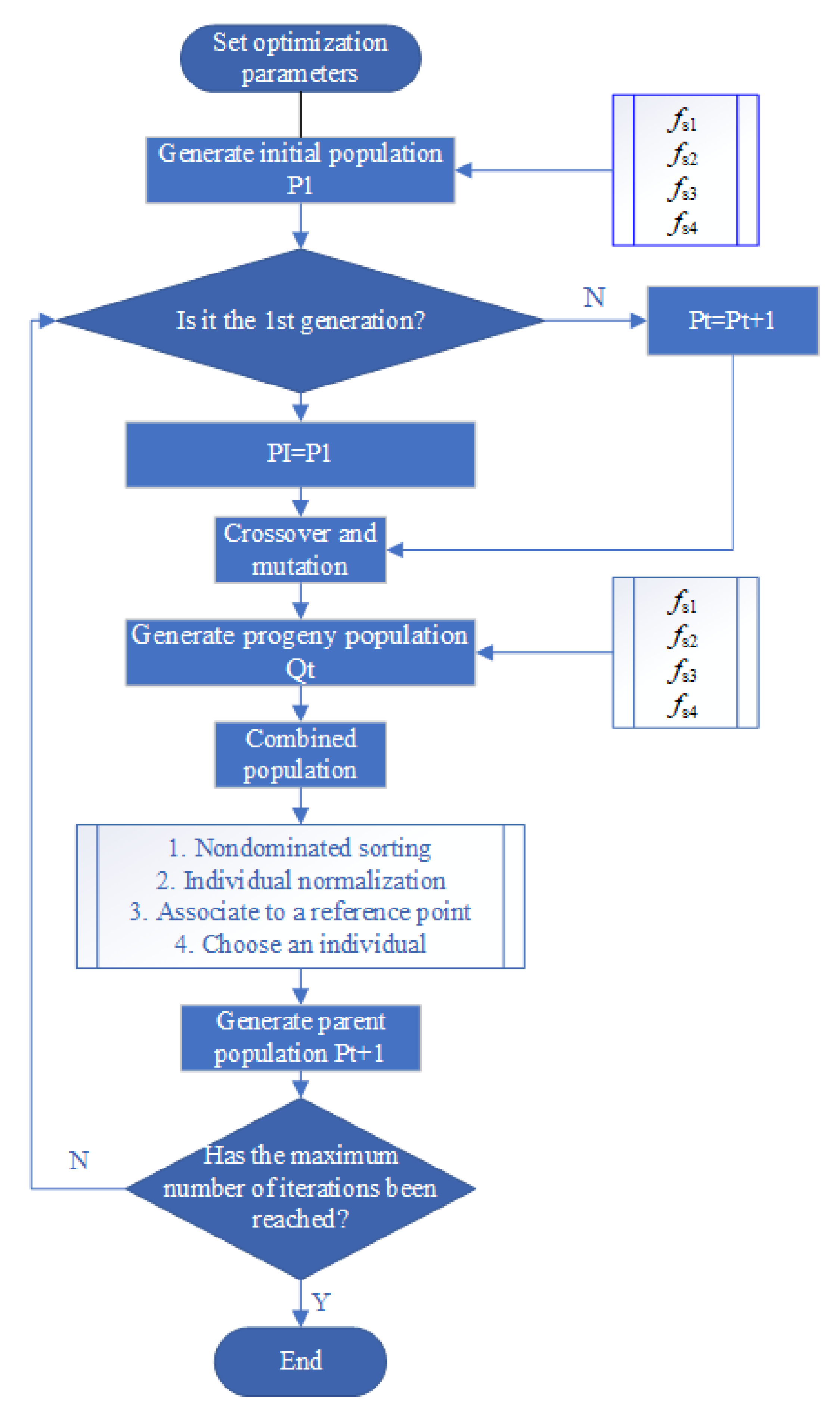
2.4. Many-Objective Optimization Algorithm NSGA-III

To improve the performance of the optimization algorithm in the many-objective optimization problem, Deb et al. [22] proposed the NSGA-III algorithm in 2014. The framework of NSGA-III is basically the same as that of NSGA-II, and it uses fast nondominated sorting to classify the population into different nondominated frontiers. The selection of the nondominated layer of the NSGA-III is different. NSGA-II used crowded comparison operations to maintain the diversity of the population, but NSGA-III used well-distributed reference points to maintain population diversity. The detailed algorithm is provided in Appendix A.

The four GPR surrogate models were embedded into NSGA-III as objective functions. With the iterating of the NSGA-III, the set of non-dominated solutions $x^{*}$ were added to the sample set to improve the generalization ability of the surrogate model on the Pareto frontier. The samples addition process can be expressed as:

$${\mathrm{D}}_{\mathrm{iter}}={\mathrm{D}}_{\mathrm{iter}-1}\cup \left[x_{\mathrm{iter} }^{*},f\left(x_{\mathrm{iter}}^{*}\right)\right].$$

(25)

The surrogate-assisted optimization process is shown in Figure 6.

3. Results and Discussion

The initial sample set (I = 88) was generated by a sampling method, and the sample set size increased as non-dominated solutions were added to the sample set, and the final sample set size was 616. The settings of NSGA-III are shown in

Table 4. Settings of NSGA-III.

Option	Value
Reference point number	50
Number of iterations	100
Population size	100
Crossover percentage	50%
Mutation percentage	50%
Mutation rate	0.02
Mutation step	0.5

.

3.1. The Simulation Results

Figure 7 shows the variation in μ with an increase in the tank pressure. When the tank pressure decreases from 101 to 90 kPa, μ decreases from 0.48 to 0.083 by 82.7%. When the tank pressure decreases from 90 to 70 kPa, μ decreases from 0.083 to 0.037 by 55.42%. When the tank pressure is lower than 80 kPa, the decaying trend of μ becomes smooth. Owing to the decreasing of the tank pressure, the velocity of nitrogen at the nozzle decreases sharply, and the eject coefficient μ decreases correspondingly. At the beginning of the vacuuming processes, the vacuuming speed of the ejector decreased rapidly with a decrease in tank pressure.

When the intermediate pressure p_s is 40 kPa, the total vacuuming time is gradually shortened with an increase in the differential pressure drop rate of the element ($\delta sp$) as shown in Figure 8. When $\delta sp$ is −1.8 Pa/s, the pump speed of the ejector is lower than that of the liquid ring pump, i.e., the ejector does not play a major role in the whole vacuum process, which means that the large pump speed feature of the ejector is not well utilized. When $\delta sp$ is 0.26 Pa/s, the pressure drop curve of the intermediate pressure transition point is smooth. With the increase in $\delta sp$, the pump speed of the ejector increases gradually, and the ejector plays an important role in the vacuuming process, and the total vacuuming time is greatly saved.

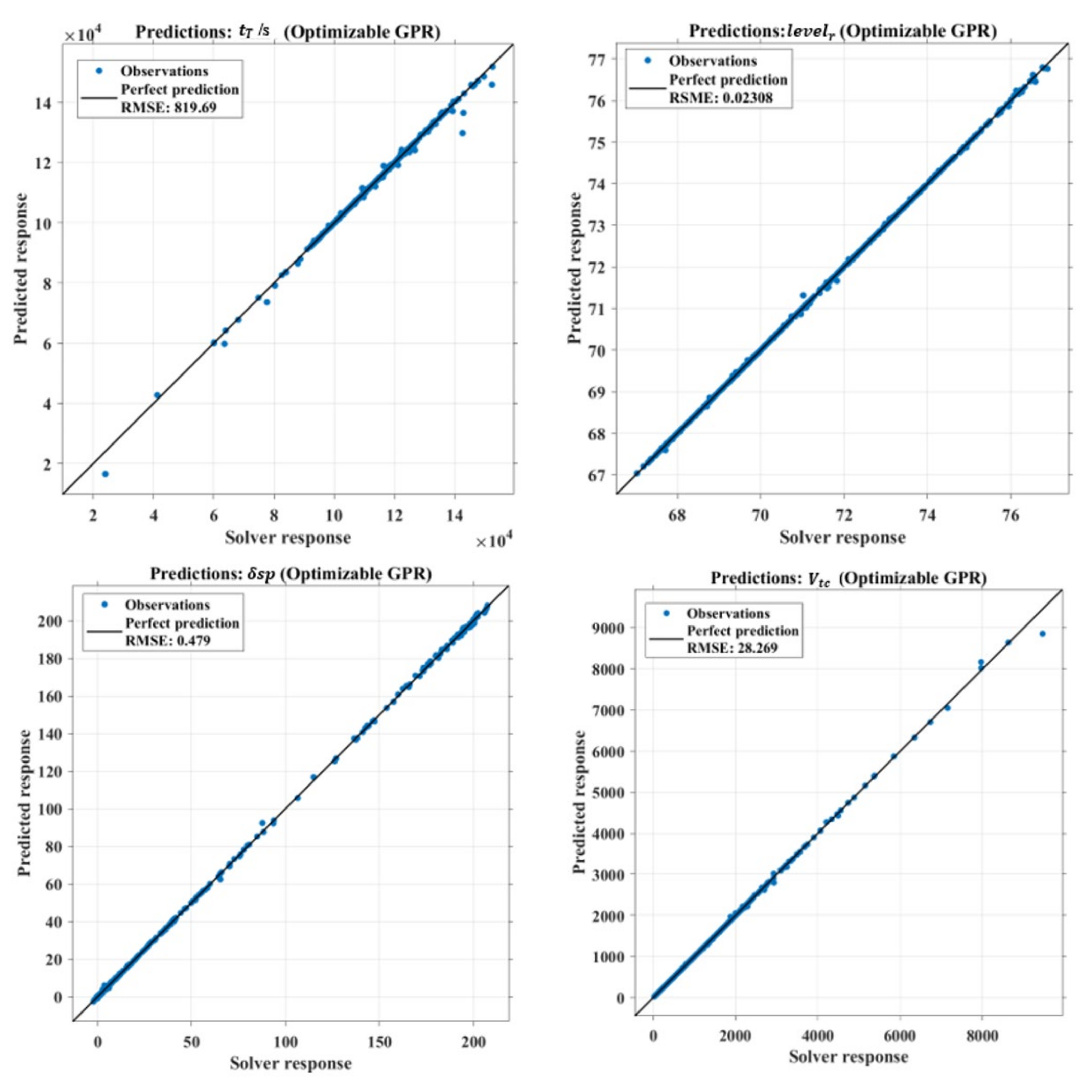
3.2. Surrogate Model Performance

The performance of the GPR optimized by Bayesian optimization is shown in Figure 9, which illustrates the prediction of GPR with the simulation results of the solver. The black line represents perfect prediction. When the observed results are closer to the black line, the prediction results are more accurate. As non-dominated solutions are added to the sample set in each generation, the prediction accuracy for GPR is gradually improved by optimizing the hyperparameter. The results showed that it takes 0.045 s for GPR to predict the simulation results, whereas the simulation of the solver takes 100–200 s. The prediction speed of GPR is 2000–4000 times faster than that of the simulation solver.

The optimized surrogate models showed a significant decrease in the RMSE of the prediction errors except for the $\delta sp$ model, as shown in

Table 5. The RMSE of the prediction errors.

	Original RMSE	Optimized RMSE	Improvement Rate
$t_T$	2557.6	819.69	−67.95%
$leve{l}_r$	0.0315	0.02308	−26.73%
$\delta sp$	0.42	0.479	+14.04%
$V_{tc}$	37.67	28.269	−24.95%

. However, compared to other GPRs, the$\delta sp$ model RMSE of the optimized GPR is the smallest on the final sample set (RMSE of rational quadratic GPR = 0.4946, RMSE of squared exponential GPR = 0.5796, RMSE of exponential GPR = 1.069, RMSE of optimized GPR = 0.479).

3.3. Analysis of Optimization Results

The Pareto frontier for the four optimization objectives was obtained using surrogate-assisted NSGA-III, as shown in Figure 10.

The shape of the interpolation surface of the scattered points of the 3D Pareto front is regular. It can be seen that the optimization results have converged. The solution of the Pareto front represents the optimal solution of each optimization objective under different weights, and the required working parameters can be selected from the Pareto front according to the design requirements.

Considering the limitation of the available conditions, several optimal operation conditions are listed in

Table 6. Optimizing solutions for the liquid oxygen vacuumed subcooling system.

Case	${\mathit{m}}_{{{N}}_2}$ (kg/s)	${\mathit{p}}_{{e}} \left(\mathbf{MPa}\right)$	${\mathit{p}}_{{s}}$ (kPa)	$\mathit{l}\mathit{e}\mathit{v}\mathit{e}{\mathit{l}}_{{i}{n}{i}{t}} (\%)$	${\mathit{s}}_{{p}}$ (m3/min)	${\mathit{t}}_{{T}}$ (s)	$\mathit{l}\mathit{e}\mathit{v}\mathit{e}{\mathit{l}}_{{r}} (\%)$	$\mathit{\delta }\mathit{s}\mathit{p}$ (Pa/s)	${\mathit{V}}_{{t}{c}}$ (Nm3)
1	1	5	16.56	86.97	15.05	65,968	70.75	1.16	2152.42
2	1	5	16.09	91.99	12.96	71,756	74.84	1.18	2267.3
3	1	5	19.45	92.95	13.25	84,127	75.54	2.02	1350.9

. The bounds on the optimization objective are the total vacuum time ($t_{\mathrm{T}}$) of less than 24 h and the nitrogen consumption of less than 2300 Sm³.

As shown in Table 6, $m_{{\mathrm{N}}_2}$ and $p_{\mathrm{e}}$ are located at the upper sampling limit of 1 kg/s and 5 MPa, and the intermediate pressure $p_{\mathrm{s}}$ is approximately near 20 kPa, which indicates that the ejector is the dominant factor in the vacuum process, and the liquid ring pump plays a supplementary role after the high-pressure nitrogen is depleted. The working conditions of Case1 represent the global shortest total vacuum time scheme, and the vacuuming time is 65,968 s (18.32 h), and the remaining liquid level is 70.75%. The working conditions of Case2 represent the trade-off scheme of total vacuuming time and remaining liquid level. The vacuuming time of Case2 is 19.93 h, which is 8.77% longer than that of Case1, and the remaining liquid level is 4.09% higher than that of Case1. The optimal solution of Case3 represents the scheme with the global maximum remaining liquid level, which is 75.54% and is 0.7% higher than that of Case2, and the vacuum time is 23.38 h and 17.3% longer than that of Case2.

3.4. Pearson Correlation Analysis

The Pearson correlation coefficient is the most commonly used correlation analysis method. For columns X_a and X_b in matrix X, ${\overline{X}}_a=\sum _{i=1}^n(X_{ai})/n,{\overline{X}}_b=\sum _{j=1}^n(X_{bi})/n,n$ is the length of each column, and Pearson’s correlation coefficient rho(a, b) is defined as:

$$rho(a,b)=\frac{{\displaystyle \sum _{i=1}^n(X_{a,i}-{\overline{X}}_a)(X_{b,i}-{\overline{X}}_b)}}{{\left\{{\displaystyle \sum _{i=1}^n{(X_{a,i}-{\overline{X}}_a)}^2{\displaystyle \sum _{j=1}^n{(X_{b,i}-{\overline{X}}_b)}^2}}\right\}}^{1/2}} .$$

(26)

The Pearson’s correlation coefficient varies from −1 to +1. If the rho(a, b) is −1, there is a completely negative correlation between a and b. If the rho(a, b) is +1, it presents a completely positive correlation between a and b. If the rho(a, b) is zero, there exists no correlation between the columns. Pearson correlation analysis was performed on the sample set, and the detailed results are given in Appendix B.

The p_s is the independent variable that has the greatest correlation with total vacuum time $t_{\mathrm{T}}$, and the Pearson’s correlation coefficient is 0.71. Because the p_s determines the vacuuming time of the ejector, it influences the total vacuuming time greatly. The vacuuming time of the ejector increases with a decrease in the p_s, and the total vacuuming time is shortened due to the relatively high vacuuming speed of the ejector. It can also be found that the vacuuming speed of the liquid ring pump is negatively related to the total vacuum time. The correlation coefficient between level_r and level_init is the highest value of 0.99, and there is a strong positive linear relationship between level_r and level_init. The pump speed of the liquid ring pump (s_p) is negatively correlated with the remaining liquid level $leve{l}_{\mathrm{r}}$ (−0.49), because the vacuuming process with the liquid ring pump in a low vacuuming speed causes a large amount of gas to be exhausted. More liquid oxygen evaporates, resulting in a decrease in the remaining liquid level. The greatest correlation coefficient between the $\delta sp$ and $p_{\mathrm{s}}$ is 0.83. The $p_{\mathrm{s}}$ is the intermediate pressure at which the vacuuming ejector is replaced by the liquid ring pump. Because of the rapid attenuation of the pumping speed of the ejector, there exists an obvious disturbance caused by the pump speed difference between the two vacuuming devices. The nitrogen consumption has a very small positive correlation with the nitrogen mass flow $m_{{\mathrm{N}}_2}$, and it has a negative correlation with the nitrogen pressure $p_{\mathrm{e}}$ (−0.194). The higher nitrogen pressure may induce the lower nitrogen consumption in the vacuuming process. The greatest negative correlation between $V_{\mathrm{tc}}$ and $p_{\mathrm{s}}$ is −0.83. The nitrogen consumption is directly related to the working time of the ejector. The smaller $p_{\mathrm{s}}$ means the working of the ejector is prolonged, and the nitrogen consumption increases correspondingly.

4. Conclusions

To improve the efficiency of a liquid oxygen vacuumed subcooling system, a vacuum system with a combination of a liquid ring pump and an ejector was employed to shorten the total vacuuming time and increase the yield of subcooled liquid oxygen. The heat and mass balances involved in the vacuuming process were simulated using a quasi-equilibrium infinitesimal method. The simulation results were compared with experimental data to verify the reliability of the simulation method. A data-driven surrogate-assisted multi-objective optimization framework was used to accelerate the optimization process of vacuum subcooling. After the regression accuracies of several surrogate models were compared, GPR was used as the best surrogate model. Bayesian hyperparameter optimization significantly improved the regression accuracy of GPR and was embedded in the NSGA-III algorithm to obtain the Pareto front. The Pearson correlation coefficient method was used to analyze the correlation between the optimization variables and the optimization objectives.

The trade-off scheme has more advantages in total vacuuming time and remaining liquid level. It can obtain the subcooled liquid oxygen at 10 kPa and 73 K with a remaining liquid level of 74.84% in the total vacuum time of 19.93 h, which greatly improves the efficiency of the liquid oxygen vacuumed subcooling system. The optimization results show that the vacuum ejector should be used to vacuum the liquid oxygen tank from atmospheric pressure to 20 kPa. Liquid ring pump only plays a supplementary role after the nitrogen is exhausted.

After the correlation analysis of the dataset, it is shown that there is a strong linear correlation between the initial liquid level and the remaining liquid level. The vacuum subcooling time has a strong linear correlation with the operating time of the ejector. Thus, the sufficient storage of high-pressure nitrogen can significantly reduce the total vacuum subcooling time and lead to an increase in the energy consumption and equipment footprint. Therefore, the trade-off solutions of multi-objective optimization is necessary.

References

1. Pengfei, A.D. Cryogenic Filling System for Launch Site of Launch Vehicle; Beijing Institute of Space Launch Technology: Beijing, China, 2011. [Google Scholar]
2. Xie, F.; Li, Y.; Wang, L. Study on subcooled technology for cryogenic propellants. J. Aerosp. Power 2017, 32, 762–768. [Google Scholar]
3. Xie, F.; Li, Y.; Wang, L.; Lei, G. Analysis on utilization of cooling capacity for ground loading system of cryogenic propellants. J. Astronaut. 2016, 37, 1381–1387. [Google Scholar]
4. Fehling, N.W. Liquid Cryogenic System; Cryogenic Engineering Editorial Department: Beijing, China, 1993. [Google Scholar]
5. Tomsik, T. Performance tests of a liquid hydrogen propellant densification ground support system for the X33/RLV. In Proceedings of the 33rd AIAA/ASME/ASEE Joint Propulsion Conference & Exhibit, Reston, VA, USA, 6–9 July 1997. [Google Scholar]
6. Lak, T.; Lozano, M.; Neary, D. Propellant densification without use of rotating machinery. In Proceedings of the 38th AIAA/ASME/SAE/ASEE Joint Propulsion Conference & Exhibit, Indianapolis, IN, USA, 7–10 July 2002; p. 2976. [Google Scholar]
7. SpaceX Announces Possible Cause of Falcon 9 Explosion on September 1. Available online: https://www.popularmechanics.com/space/rockets/a23020/spacex-rocket-explosion-cause/ (accessed on 18 October 2021).
8. Zuo, Z.; Jiang, W.; Pan, P.; Qin, X.; Huang, Y. Quasi-equilibrium evaporation characteristics of oxygen in the liquid–vapor interfacial region. Int. Commun. Heat Mass Transf. 2021, 129, 105697. [Google Scholar] [CrossRef]
9. Safari, F.; Dincer, I. Assessment and optimization of an integrated wind power system for hydrogen and methane production. Energy Convers. Manag. 2018, 177, 693–703. [Google Scholar] [CrossRef]
10. Khan, M.S.; Karimi, I.; Lee, M. Evolution and optimization of the dual mixed refrigerant process of natural gas liquefaction. Appl. Therm. Eng. 2016, 96, 320–329. [Google Scholar] [CrossRef]
11. Song, R.; Cui, M.; Liu, J. Single and multiple objective optimization of a natural gas liquefaction process. Energy 2017, 124, 19–28. [Google Scholar] [CrossRef]
12. Mofid, H.; Jazayeri-Rad, H.; Shahbazian, M.; Fetanat, A. Enhancing the performance of a parallel nitrogen expansion liquefaction process (nelp) using the multi-objective particle swarm optimization (mopso) algorithm. Energy 2019, 172, 286–303. [Google Scholar] [CrossRef]
13. Díaz-Manríquez, A.; Toscano, G.; Barron-Zambrano, J.H.; Tello-Leal, E. A review of surrogate assisted multiobjective evolutionary algorithms. Comput. Intell. Neurosci. 2016, 2016, 1–14. [Google Scholar] [CrossRef] [PubMed] [Green Version]
14. Tan, H.; Zhao, Q.; Sun, N.; Li, Y. Enhancement of energy performance in a boil-off gas re-liquefaction system of LNG carriers using ejectors. Energy Convers. Manag. 2016, 126, 875–888. [Google Scholar] [CrossRef]
15. Viana, F.A.C.; Venter, G.; Balabanov, V. An algorithm for fast optimal Latin hypercube design of experiments. Int. J. Numer. Methods Eng. 2010, 82, 135–156. [Google Scholar] [CrossRef] [Green Version]
16. Neter, J.; Kutner, M.H.; Nachtsheim, C.J.; Wasserman, W. Applied Linear Statistical Models; IRWIN, The McGraw-Hill Companies, Inc.: Martinsville, OH, USA, 1996. [Google Scholar]
17. Breiman, L.; Friedman, J.; Olshen, R.; Stone, C. Classification and Regression Trees; CRC Press: Boca Raton, FL, USA, 1984. [Google Scholar]
18. Schölkopf, B.; Mika, S.; Burges, C.J.C.; Knirsch, P.; Muller, K.R.; Ratsch, G.; Smola, A.J. Input space versus feature space in kernel-based methods. IEEE Trans. Neural Netw. 1999, 10, 1000–1017. [Google Scholar] [CrossRef] [PubMed] [Green Version]
19. Rasmussen, C.E.; Williams, C.K.I. Gaussian Processes for Machine Learning; MIT Press: Cambridge, MA, USA, 2006. [Google Scholar]
20. Lucchese, C.; Nardini, F.M.; Orlando, S.; Perego, R.; Tonellotto, N.; Venturini, R. A Fast algorithm to rank documents with additive ensembles of regression trees. In Proceedings of the 38th International ACM SIGIR Conference on Research and Development in Information Retrieval, Santiago, Chile, 9–13 August 2015; pp. 73–82. [Google Scholar]
21. Li, L.; Jamieson, K.; DeSalvo, G.; Rostamizadeh, A.; Talwalkar, A. Hyperband: A novel bandit-based approach to hyperparameter optimization. J. Mach. Learn. Res. 2018, 18, 6765–6816. [Google Scholar]
22. Deb, K.; Jain, H. An Evolutionary Many-Objective Optimization Algorithm Using Reference-Point-Based Nondominated Sorting Approach, Part I: Solving Problems with Box Constraints. Evolutionary Computation. IEEE Trans. 2014, 18, 577–601. [Google Scholar] [CrossRef]
Figure 1. Ejector/liquid ring pump vacuum subcooling system.
Processes 10 01188 g001
Figure 2. Schematic diagram of the liquid-nitrogen vacuumed subcooling system.
Processes 10 01188 g002
Figure 3. Image of the liquid nitrogen vacuumed subcooling test set.
Processes 10 01188 g003
Figure 4. Comparison of simulation and experimental data: (a) tank pressure deviation and (b) tank liquid level deviation.
Processes 10 01188 g004
Figure 5. Bayesian optimization process.
Processes 10 01188 g005
Figure 6. Optimization process of surrogate-assisted NSGA-III.
Processes 10 01188 g006
Figure 7. The variation of µ with the tank pressure.
Processes 10 01188 g007
Figure 8. Pressure drop curve for different δ s p .
Processes 10 01188 g008
Figure 9. Final surrogate model performance.
Processes 10 01188 g009
Figure 10. Pareto frontier of surrogate model.
Processes 10 01188 g010