Article

Optimal Control Strategy of Path Tracking and Braking Energy Recovery for New Energy Vehicles

1
School of Transportation and Vehicle Engineering, Shandong University of Technology, Zibo 255049, China
2
Hubei Key Laboratory of Power System Design and Test for Electrical Vehicle, Hubei University of Arts and Science, Xiangyang 441053, China
*
Author to whom correspondence should be addressed.
Processes 2022, 10(7), 1292; https://doi.org/10.3390/pr10071292
Submission received: 22 May 2022 / Revised: 21 June 2022 / Accepted: 22 June 2022 / Published: 30 June 2022

Abstract

:
In order to further improve the stability of path tracking control and fuel economy of new energy vehicles, an optimal control strategy of path tracking and braking energy recovery is proposed. First, a model predictive controller is designed based on the three-degrees of freedom dynamics model of the vehicle according to the idea of hierarchical control, and a fuzzy yaw torque controller is established with the desired yaw velocity and side slip angle of the mass center as constraints. Second, at high-speed driving conditions, the executive layer of the component distributes the braking torque according to the braking energy recovery control strategy. Finally, the optimal control strategy of path tracking and braking energy recovery is verified by Carsim/Advisor/Simulink software under different driving speeds. The results show that the optimized control strategy can improve the tracking accuracy and driving stability of a vehicle with large curvature turning and further improve the fuel economy of new energy vehicles under the premise of meeting the control requirements.

1. Introduction

With the lag of transportation construction development and the rapid increase in the number of vehicles, the problems of traffic congestion, vehicle travel safety, automobile energy conservation, and emission reduction have become a concern of the government and the general public. In addition, unreasonable urban road planning also causes traffic congestion problems. Therefore, the development of intelligent vehicles and new energy vehicles has become a top priority, and the optimization control of vehicle motion is a key technology for driverless vehicles. In addition, the problem of global warming is becoming more and more serious. However, vehicle exhaust emissions are one of the important factors causing environmental pollution. Developing new energy vehicles has become the consensus of all countries. At present, there are many control algorithms, such as the pure tracking algorithm of a geometric model, but the tracking effect is not good when the vehicle speed is too high [1,2]. A PID (Proportion Integration Differentiation) algorithm can control the vehicle lateral error according to the trajectory deviation, but the adjustment of parameters under different working conditions is the disadvantage of the algorithm [3,4,5]. A linear quadratic regulator (LQR) takes into account the influence of the vehicle dynamics model, but requires higher accuracy of the vehicle model [6,7,8,9,10]. Lghani Menhour [11] proposed a mathematical driver model based on a two-degrees-of-freedom PID multi-controller, developed a mathematical driver model, and verified the robustness and stability of the control, which improved the control accuracy under the uncertainty of nonlinear and structured parameters. This method effectively evaluated the driving limit of vehicles under curve conditions. Toshihiro Hiraoka [12] proposed an automatic 4WS (four-wheel steer) controller based on the sliding-film theory. The controller is robust to steering power disturbance, target path radius variation, and lateral force disturbance. Penglei Dai and Jay Katupitiya [13] proposed a novel control method for four-wheel steering and four-wheel drive (4WS4WD) vehicles. The sliding mode control (SMC) and particle swarm optimization (PSO) are integrated to solve the control problem of the nonlinear and highly coupled four-wheel steering system.
Compared with the above traditional methods, the model predictive control method has the ability to systematically consider the prediction information. The future output behavior of the system can be predicted by the rolling time domain control method and converted into solving the constrained optimal control problem. In 2005, Italy’s Falcone [14] proposed front-wheel steering control based on the model prediction algorithm, so the vehicle can track the desired path root under the condition of satisfying the physical constraints. This method considers the dynamic characteristics and physical constraints of the vehicle and can continuously optimize the control parameters. Duan [15] improved the accuracy of intelligent vehicle path tracking by improving the objective function, increasing the dynamic constraint of tire cornering, and using the vehicle dynamic model as the prediction model of model predictive control. Zhang [16] analyzed the relationship between vehicle speed and prediction time domain, fitted the function curve of prediction time domain and vehicle speed, and designed a variable time domain adaptive path tracking controller so that the vehicle can update the prediction time domain in real time and ensure the vehicle has good tracking accuracy and stability. However, the above methods are designed under the assumption that the vehicle sideslip characteristics are linear, and the uncontrolled problem caused by the sideslip characteristics entering the nonlinear region at high speed is not considered.
With an increasing number of vehicles, how to save energy and reduce emissions have become the research objectives of many scholars. Guangdong Tian analyzed the reuse of abandoned vehicles in China and put forward a series of methods to improve processing efficiency [17,18,19]. In addition, energy vehicles using clean energy are also research hotspots. With the development of electric vehicles, the shortcomings of electric vehicles have also been amplified. Because the charging stations of electric vehicles are only present in some big cities and highway service stations, it causes difficulty in charging pure electric vehicles, and the owners are anxious about the endurance of electric vehicles. Compared with traditional internal combustion engines, the exhaust emission of hybrid vehicles is greatly reduced [20,21]. Braking energy recovery can improve energy reuse and reduce vehicle cost. Many experts have studied braking force distribution at the energy management level to improve braking energy recovery potential and reduce fuel consumption [22,23,24]. There are many braking modes in the braking process, and the smoothness of braking control is a major research focus [25,26,27]. How to maintain the stability of ABS (antilock brake system) while considering the braking distribution is the key point. Different from the traditional braking mode, the coordinated control of motor and mechanical braking can ensure the safety of vehicles to the greatest extent [28,29,30,31,32,33,34,35,36]. Some studies apply intelligent control and optimization algorithms to vehicle control strategies [37,38,39,40]. Based on the current research status, braking force collaborative control under emergency conditions still needs to be solved urgently. The instability problem of vehicle path tracking at high speed and the coordinated control of braking force under emergency conditions are also research hotspots. In addition, there are few or no studies considering both. In view of the above problems, this paper designs an optimal control strategy as follows.
From the perspective of vehicle intelligence and energy saving, the paper proposes a path tracking and braking energy recovery optimization control strategy for new energy vehicles. First, a three-degrees-of-freedom vehicle dynamics model is established, and on this basis, a model predictive controller is established. In view of the tracking instability problem, a reference model based on the steady-state response of the vehicle is established. The tire sideslip characteristics are controlled in a linear range by setting the boundary value. The fuzzy yaw moment controller is established by taking the error between the vehicle state and the reference model as the input and the additional yaw moment as the output. The expected braking torque is calculated according to the vehicle torque distribution. Finally, the fuzzy controller is established by taking the current vehicle speed, braking force, and battery state of charge (SOC) as the inputs to calculate the motor braking ratio. The expected braking torque is divided into hydraulic braking and motor braking to achieve vehicle stability control and braking energy recovery.
The rest of this paper is as follows. The overall structure of the control strategy is presented is Section 2. The vehicle dynamics model and the path tracking stability control strategy is designed in Section 3. The braking energy recovery strategy is designed in Section 4. The simulation results are provided in Section 5, followed by the concluding remarks in Section 6.

2. Overall Architecture of the Control System

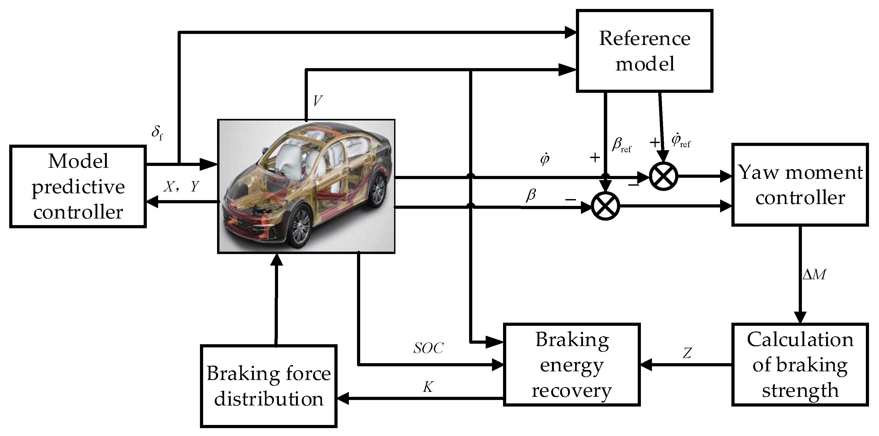
The overall control structure is shown in Figure 1. The control system is divided into seven parts: model predictive controller, reference model, yaw moment controller, braking strength calculation module, fuzzy braking energy recovery controller, braking force distributor, and hybrid electric vehicle. The model predictive controller calculates the required front wheel angle according to the current position of the vehicle. The reference model calculates the expected value of the sideslip angle of the centroid and the expected value of the yaw rate according to the steady-state response formula of the vehicle with two degrees of freedom. The value is taken as the control objective, and the yaw moment controller is built to output the required additional yaw moment. The braking torque is calculated by the braking strength calculation module, and the regenerative braking ratio is calculated by fuzzy control. The hydraulic braking torque and regenerative braking torque are output by the braking force distribution system.
Figure 1 is the control system structure, where δ f is the front wheel expert, X, Y are the current vehicle lateral and longitudinal positions, V is the current speed, φ ˙ and φ ˙ nef are the yaw rate and yaw rate expectations, β and β nef are the sideslip angle and sideslip angle expectations, Δ M is the additional yaw moment, Z is the braking strength, K is the regenerative braking ratio, and SOC is the battery state of charge.
The control strategy is divided into two layers as a whole. The upper controller calculates the vehicle front wheel angle of the path tracking according to the current vehicle deviation and vehicle speed and calculates the expected yaw rate and sideslip angle under the current vehicle speed and the front wheel angle. The additional yaw moment is calculated with the expected value as the control objective. The lower controller calculates the required braking torque according to the vehicle torque balance relationship and calculates the regenerative braking ratio under the current braking strength, vehicle speed, and SOC by the fuzzy controller. Finally, the hydraulic braking torque and motor braking ratio are output according to the braking ratio.

3. Design of Stability Control Strategy for Path Tracking

3.1. Vehicle Dynamic Model

According to the model requirements of MPC, two-wheel three-degrees-of-freedom vehicle model is selected as the research object. It is assumed that the left and right angles of the front wheel are equal, and the load transfer caused by suspension or accelerated braking is ignored. Based on the above assumptions, the vehicle longitudinal axis is set as the X axis, the vehicle transverse axis is the Y axis, the vehicle centroid perpendicular to the XOY plane is the Z axis, and the vehicle longitudinal, transverse, and yaw motions on the three axes are analyzed, respectively. The dynamic model of the vehicle with two wheels and three degrees of freedom is shown in Figure 2.
Longitudinal force of the vehicle in the X-axis direction:
m x ¨ = m y ¨ φ ˙ + 2 F xf + 2 F xr
Lateral force of the vehicle in the Y-axis direction:
m y ¨ = m x ˙ φ ˙ + 2 F yf + 2 F yr
Yaw moment of vehicle in Z-axis direction:
I z φ ¨ = 2 a F yf 2 b F yr
where m is the vehicle’s spare mass, and a and b are the distance between the vehicle’s center of mass and the front and rear axles, respectively.
According to the calculation of mechanical and geometric relations, the transverse and longitudinal forces of the tire are as follows:
F xf = F lf cos δ f F cf sin δ f
F xr = F lr cos δ r F cr sin δ r
F yf = F lf sin δ f + F cf cos δ f
F yr = F lr sin δ r + F cr cos δ r
According to the coordinate relation, the sideslip angle of the front and rear tires can be approximately expressed as:
α f = y ˙ + a φ ˙ x ˙ δ f
α r = y ˙ a φ ˙ x ˙
The vehicle speed in the inertial coordinate system needs to be obtained according to the conversion relationship between it and the vehicle coordinate system, and the formula is as follows:
Y ˙ = x ˙ sin φ + y ˙ cos φ
X ˙ = x ˙ cos φ y ˙ sin φ
Formulas (4)–(11) are substituted into Formulas (1)–(3) to obtain the three-DOF dynamics model of the second wheel of the vehicle:
{ m y ¨ = m x ˙ φ ˙ + 2 [ C cf ( δ f y ˙ + a φ ˙ x ˙ ) + C cr b φ ˙ y ˙ x ˙ ] m x ¨ = m y ˙ φ ˙ + 2 [ C lf s f + C cf ( δ f y ˙ + a φ ˙ x ˙ ) δ f + C lr S r ] I z φ ¨ = 2 [ a C cf ( δ f y ˙ + a φ ˙ x ˙ ) b C cr b φ ˙ y ˙ x ˙ ] Y ˙ = x ˙ sin φ + y ˙ cos φ X ˙ = x ˙ cos φ y ˙ sin φ
where Ccf, Ccr are, respectively, the lateral stiffness of front and rear tires of the vehicle; Clf, Clr are the longitudinal stiffness of front and rear tires; Sf, Sr are front and rear wheel slip rates, respectively; δf is front wheel rotation angle; X and Y are the longitudinal and transverse positions of the vehicle in the inertial coordinate system, respectively, relative to the corresponding longitudinal velocity and transverse velocity.

3.2. Design of Model Predictive Tracking Controller

According to Formula (12), the equation of state based on nonlinear dynamics model is established:
ξ ˙ = f ( ξ , u )
The state quantity is ξ = [ y ˙ , x ˙ , φ , φ ˙ , Y , X ] T , and the control quantity is u = δ f . The nonlinear equation of state is expanded at ( ξ r , u r ) by Taylor’s formula, and the higher-order terms are ignored and only the first-order terms are retained:
ξ ˙ = f ( ξ r , u r ) + f ξ | ξ = ξ r u = u r ( ξ ξ r ) + f u | ξ = ξ r u = u r ( u u r )
Equation (14) can be subtracted from Equation (13) to obtain the state equation of error:
Δ ξ ˙ = A ( t ) Δ ξ + B ( t ) Δ u
In the equation:
Δ ξ = ξ ξ r ,   Δ u = u u r ,   A ( t ) = f ξ | ξ = ξ r u = u r ,   B ( t ) = f u | ξ = ξ r u = u r
The coefficients A(t), B(t) of the new equation of state are as follows:
A ( t ) = [ 2 ( C cf + C cr ) m x ˙ t f y ˙ x ˙ 0 x ˙ t + 2 ( b C cr a C cf ) m x ˙ t 0 0 φ ˙ 2 C cf δ f , t 1 m x ˙ f x ˙ x ˙ 0 y ˙ 2 a C cf δ f , t 1 m x ˙ t 0 0 0 0 0 1 0 0 2 ( b C cr a C cf ) I z x ˙ t f φ ˙ x ˙ 0 2 ( a 2 C cf + b 2 C cf ) I z x ˙ t 0 0 cos ( φ t ) sin ( φ t ) x ˙ t cos ( φ t ) y ˙ t sin ( φ t ) 0 0 0 sin ( φ t ) cos ( φ t ) y ˙ t cos ( φ t ) x ˙ t sin ( φ t ) 0 0 0 ]
B ( t ) = [ 2 C cf m 2 C cf ( 2 δ f , t 1 y ˙ t + a φ ˙ t x ˙ t ) m 0 2 a C cf I z 0 0 ]
f x x ˙ = 2 C cf δ f , t 1 ( y ˙ t + a φ ˙ t ) m x ˙ t 2 ,   f φ ˙ x ˙ = 2 a C cf ( y ˙ t + a φ ˙ t ) 2 b C cr ( y ˙ t b φ ˙ t ) I z x ˙ t 2
According to the recursive calculation requirements of MPC, the equation of state is discretized and the following formula is obtained:
{ A ( k ) = I + T A ( t ) B ( k ) = T B ( t )
Combining Equations (15) and (16), the linearly discretized equation of state can be obtained:
Δ ξ ( k + 1 ) = A k Δ ξ ( k ) + B k Δ u ( k )

3.2.1. Transformation of State Space Equations

In order to take the front wheel rotation angle and its variation as the controlled target, the linearized state space equation should be transformed and set:
ξ ( k ) = [ Δ ξ ( k ) u ( k ) ] ,   η ( k ) = C ξ ( k ) ,
The transformed equation of state is obtained by combining the new state quantity and control increment:
ξ ( k + 1 ) = A ˜ ξ ( k ) + B ˜ Δ u ( k ) η ( k ) = C ˜ ξ ( k )
In Equation (18),
A ˜ ( k ) = [ A k B k 0 I ] ;   B ˜ ( k ) = [ B k I ] ;   C ˜ = [ C k 0 ] ;   Δ u ( k ) = u ( k ) u ( k 1 )
Starting from K = 1, the formula is respectively deduced to Nc (control time domain) and Np (prediction time domain), and the P line formula is obtained, which is expressed in the form of state space equation:
Y ( k + 1 ) = Ψ ξ ( k ) + Θ Δ U ( k )
Ψ = [ C ˜ k A ˜ k C ˜ k A ˜ k 2 C ˜ k A ˜ k N p ] ,   Θ = [ C ˜ k B ˜ k 0 0 C ˜ k A ˜ k B ˜ k C ˜ k B ˜ k 0 C ˜ k A ˜ k N c 1 B ˜ k C ˜ k A ˜ k N c 2 B ˜ k C ˜ k B ˜ k C ˜ k A ˜ k N c B ˜ k C ˜ k A ˜ k N c 1 B ˜ k C ˜ k A ˜ k B ˜ C ˜ k A ˜ k N p 1 B ˜ k C ˜ k A ˜ k N p 2 B ˜ k C ˜ k A ˜ k N p N c 1 B ˜ k ]

3.2.2. Objective Function

The objective function of the tracking error is expressed as follows:
J ( ξ ( t ) , u ( t 1 ) , Δ U ( t ) ) = i = 1 N p η ( t + i | t ) η ref ( t + i | t ) Q 2 + i = 1 N c 1 | | Δ u ( t + i | t ) | | R 2 + ρ ε 2
where Q is the weight coefficient of the state quantity; R is the weight coefficient of the control quantity; ρ is the weight coefficient of the relaxation factor; and ηref is the reference value of the output.
After the above deduction, the model prediction problem is transformed into a quadratic programming solution problem:
min J ( ξ ( t ) , u ( t 1 ) , Δ U ( t ) ) , s . t . U min A Δ U t + U t U max , Δ U min Δ U Δ U max , y h . min y h y h . max , y s , min + ε y s y s , max + ε .
In each calculation cycle of the quadratic programming solution, the control input within the constraint range is:
Δ U t * = [ Δ u t * , Δ u t + 1 * , Δ u t + N c 1 * , ε ] T
In the above formula, the element in the first row of the matrix is the change value of the control quantity, which is added with the initial control quantity to obtain the actual control quantity corresponding to the period:
u ( t ) = u ( t 1 ) + Δ u t *
When the system repeats this process, the control quantity will change with the change of the path trajectory, and the closed-loop tracking control will be realized for the desired trajectory.

3.2.3. Constraint Condition

Because the selection of sideslip angle and tire sideslip angle play a crucial role in vehicle steering stability, according to the research results of Bosch Company, the limit value of the sideslip angle is set to 12°, the extreme value of tire sideslip linear angle is set to 5°.

3.2.4. Model Predictive Control Principle

The principle of model predictive control is shown in Figure 3. The real-time state of the vehicle is input into the MPC controller, the difference between the actual position and the reference position is calculated, and the optimization is predicted. The calculated value is input into the vehicle to realize closed-loop control.

3.3. Reference Model Design

In order to avoid instability and path tracking failure when the vehicle is turning at high speed, the vehicle will not deviate from the tracking path by limiting the stability parameters when the vehicle is turning at high speed. According to the two-DOF vehicle steady-state response model, the steady-state expected value of the vehicle is deduced:
φ ˙ nef = x ˙ / L 1 + K x ˙ 2 × δ f
β nef = b + a m x ˙ 2 / C r L ( 1 + K x ˙ 2 ) / L × δ f
K = m L 2 ( a C r b C f ) is the stability coefficient, L is the wheelbase of front and rear axles; φ ˙ nef is the steady-state value of yaw velocity; and β nef is the steady state value of the sideslip angle of centroid.
In the two-degrees-of-freedom vehicle steady-state response model, it is assumed that the tire lateral force characteristic is linearly distributed. Therefore, the paper avoids the tire exceeding the adhesion limit by setting the boundary value of the yaw rate and the centroid lateral angle so as to ensure that the tire lateral force characteristic curve is linearly distributed. The boundary values of yaw rate and sideslip angle of centroid are:
| φ ˙ b o u n d | = 0.85 μ g x ˙
| β b o u n d | tan 1 ( 0.02 μ g )

3.4. Design of Fuzzy Yaw Moment Controller

According to the controller design, the paper adopts the two-input single-output control method. According to the design requirements of fuzzy rules, the input and output are described by the language description method of {PB, PM, PS, ZO, NS, NM, NB} on the basis of practice summary. The fuzzy controller input is described by five linguistic variables, and the fuzzy subset of linguistic variables is set to {PB, PS, ZO, NS, NB}. The output language variables are described by seven language variables, and the fuzzy subset is set to {PB, PM, PS, ZO, NS, NM, NB}. According to expert experience, the fuzzy universe of input is set to [–3, 3] and the fuzzy universe of output is set to [–1, 1]. According to the requirements of fuzzification, the actual cybernetic domain and fuzzy domain are proportional. Quantization factor ke and scale factor ku are defined as follows:
k e = n 1 e
k u = u n 2
where n1 is the fuzzy theory domain of the input variable, e is the matter theory domain of the input variable, u is the matter theory domain of the output variable, and n2 is the fuzzy theory domain of the output variable. The selected quantization factor ke1 = 0.1, quantization factor ke2 = 1, and scale factor ku = 6000 of ∆M.
According to the requirements of real-time and rapidity of vehicle control, the membership function of fuzzy language variable is triangular. This kind of membership function has a sharp curve shape and high resolution and can quickly respond to the changes in the vehicle state under high-speed conditions, as shown in Figure 4 and Figure 5.
Based on expert experience and simulation verification, fuzzy rules are shown in Table 1.

3.5. Braking Force Strength Calculation and Additional Yaw Moment Control

The additional yawing moment is calculated according to the input value. At the same time, the braking strength is calculated according to the yaw moment formula in order to prevent the single wheel brake instability. Therefore, the braking force rule adopts the same-side braking mode, and the same-side braking wheels and cylinders generate the same braking pressure to provide the additional yaw moment. The braking force distribution of the brake wheel is shown in Table 2.
According to the relationship between the brake wheel cylinder pressure and the required additional yaw moment, the braking pressure can be expressed as follows:
P i = Δ M r B c i
where i = 1 represents the front cylinder and rear cylinder on the left side of the vehicle, i = 2 represents the front cylinder and rear cylinder on the right side of the vehicle, ∆M is the output of fuzzy control with additional yaw moment, r is the effective rolling radius of the tire, B is the wheel pitch between the wheels, and c is the braking moment of the unit wheel cylinder of the front and rear wheels.

4. Braking Energy Recovery Control Strategy for Hybrid Electric Vehicles

4.1. Influence Factors of Braking Energy Recovery

In the braking energy recovery process of hybrid electric vehicles, the energy recovery efficiency will be interfered with by many factors. Several factors that affect the braking energy recovery are listed below.
(1)
The motor is the core component of the braking energy recovery system. The function of the motor is to realize the energy conversion between mechanical energy and electric energy. Its advantages and disadvantages directly determine the energy recovery efficiency.
(2)
The energy storage equipment of a hybrid electric vehicle is the battery. The size of the battery SOC has a significant impact on the effect of braking energy recovery. If the battery SOC is too large, the battery capacity is not sufficient to recover excessive electrical energy. When the battery SOC is small, the battery can store more energy, which will improve the braking energy recovery efficiency.
(3)
Environmental factors and environmental conditions are also important factors affecting energy recovery in the braking process. The energy recovery efficiency of horizontal pavement is higher in good road conditions. In complex pavement, the energy recovery efficiency will be greatly reduced under conditions of water or deep pits.
(4)
Control strategy is another core of hybrid electric vehicle braking energy recovery. For hybrid electric vehicle braking energy recovery systems, a reasonable braking force distribution control strategy can improve braking energy recovery efficiency. A good control strategy can achieve more energy recovery under the premise of ensuring vehicle safety and stability.

4.2. Fuzzy Controller Design

Road traffic conditions, weather factors, driver’s driving habits, vehicle speed, and other factors may have some impact on hybrid vehicle braking energy recovery. Because the vehicle speed V, braking strength Z, and battery SOC have great influence on braking energy recovery, these three factors are selected as input signals to be applied in the fuzzy control braking energy recovery system, which is shown in Figure 6.

4.2.1. Membership Function Design

Vehicle speed is the most important parameter in the process of driving. The magnitude of the vehicle speed directly affects the braking energy recovery effect of the vehicle. When the vehicle speed is too low, the vehicle braking is mechanical braking, and the motor does not participate in braking. When the vehicle speed rises to a certain value, the proportion of motor participation will increase in the braking process. In this case, the vehicle can recover more braking energy. In Figure 7, the speed range of the vehicle is set to [0, 100] and to {L, M, H}. L, M, and H are low, medium, and high fuzzy languages, respectively. The set {L, M, H} in Figure 8 and Figure 9 are the same.
Braking strength Z is determined by the size of the driver’s pedal force. In order to consider the safety of the vehicle in the braking process, the braking strength Z also greatly affects the energy recovery efficiency of the vehicle. When the braking intensity Z is small or medium, the braking process of the vehicle slows down, the braking force demand is small, and the electric mechanism force accounts for a large proportion. In this process, the vehicle can recover more braking energy. When the braking intensity Z is large, it indicates that the driver wants emergency braking of the vehicle. At this time, the braking force of the motor is very small, and the vehicle braking energy recovery is also very small. We set the braking strength Z to [0, 1] and to {L, M, H}.
The battery is an energy storage device for hybrid electric vehicle energy recovery, and it plays a great role in the energy conversion process of braking energy recovery. The SOC value has a great influence on the charging efficiency of the hybrid electric vehicle battery. When the SOC of the battery is low, the charging of the battery is unlimited. When the SOC value is too large, it is not appropriate to charge too much electricity. We set the domain of battery SOC to [0, 1] and to {L, M, H}.
Regenerative braking ratio K represents the ratio of motor to total braking force. We set the fuzzy set of regenerative braking ratio K as [lower, low, middle, high], abbreviated as [SL, L, M, H]. In Figure 10, SL indicates that the motor does not work in the braking process of the vehicle, and the hybrid electric vehicle basically does not recover energy; L means that the braking of the motor is small; M indicates that the proportion of the braking force of the motor in the total braking force of the vehicle is medium; H indicates that in the process of automobile braking, the braking force mainly comes from the motor.

4.2.2. Fuzzy Rule

When the vehicle speed is low, the motor of the hybrid electric vehicle basically does not work and the vehicle does not recover braking energy during braking. When the vehicle speed is medium, the proportion of motor participation in vehicle braking increases; when the vehicle speed is high, the proportion of motor participation in braking is high, and the braking energy recovery is increased.
When the braking intensity Z is large, the vehicle is in an emergency braking condition. In order to ensure the safety and stability of driving, the motor is basically not involved in braking, and the braking force is all provided by the mechanical friction system. When the braking strength is small or medium, the braking force generated by the motor increases, and the recovery energy will also increase.
When the SOC value of the battery state of charge of a hybrid electric vehicle is higher, the battery surplus power is greater. In order to prevent battery overcharge and negatively affect battery life, the proportion of motor braking participation is low or not involved. When the SOC value is low, the battery capacity is sufficient to store the energy converted from braking energy, so the proportion of motor participation in braking is high. Specific fuzzy rules are designed as shown in Table 3.
Under the fuzzy control rules shown in the table, the relationship between vehicle speed V, braking strength Z, battery SOC, and regenerative braking ratio K is shown in Figure 11, Figure 12 and Figure 13. It can be seen from Figure 11 that with the increase in braking intensity Z and vehicle speed V, the regenerative braking ratio K increases first, then decreases, and finally increases.

5. Simulation Proof

In order to verify the feasibility of the algorithm, MATLAB\Simulink is used to write the control program, and the simulation experiment is completed by Carsim and Advisor. The selection of specific models and parameters is shown below.

5.1. Simulation Platform Parameter Design

Vehicle parameters, motor parameters, and battery parameters are shown in Table 4, Table 5 and Table 6.
The double-shift curve is selected as the path tracking route. The double-shift curve contains intense corner changes, which can meet the requirements of high-speed steering conditions in this paper. Therefore, based on the Carsim\Simulink co-simulation platform, using the double-shift curve as the tracking path can better detect the stability of the algorithm.

5.2. Simulation Result

In order to verify the feasibility of the controller design, the optimal control strategy of path tracking and braking energy recovery was simulated and verified under the driving conditions of 30 km/h, 50 km/h, and 70 km/h, respectively, by driving on a road surface of μ = 0.9 and ignoring the influence of wind resistance.

5.2.1. Cause Analysis of Vehicle Instability

It can be seen from Figure 14 that the MPC can track the path stably at 30 km/h and 50 km/h. However, with the increase in vehicle speed, the vehicle is out of control under the condition of 70 km/h. According to the analysis, the model predictive controller is built on the basis of the three-degrees-of-freedom dynamic model of the vehicle, and the tire sideslip characteristics are assumed to be a linear distribution, so the front wheel angle is calculated under the ideal state. In the actual control process, as the vehicle enters high-speed conditions, the sideslip angle of the tire becomes larger, and the sideslip characteristics enter the nonlinear region, which cannot provide the required tire corner force under the ideal state, resulting in the vehicle being out of control. under the ideal state, resulting in vehicle out of control.
As seen in Table 7, compared with MPC, the average error of the stability control strategy is reduced by 0.071 m and the maximum error is reduced by 0.846 m at high speed. It can be seen that the control strategy in this paper improves the accuracy of vehicle high-speed path tracking and avoids instability.

5.2.2. Control Effect Analysis of Controller

In order to verify the control effect of the controller under high-speed driving conditions, a driving condition of 70 km/h was selected for analysis, as shown in Figure 15.
By comparing the centroid sideslip angle and yaw rate of the MPC and the path tracking combined controller at 70 km/h, the sideslip angle of the path tracking combined controller is stabilized between −5°and 5°according to the requirements of the reference trajectory, which ensures steering stability under high-speed driving conditions. The MPC only controls the front wheel angle under the ideal sideslip condition. When the vehicle speed is too high, the tire sideslip characteristics enter the nonlinear region. it can be seen that the vehicle loses the yaw stability after 4 s, and the vehicle path tracking fails.
In Figure 16, the additional yaw moment image indicates that when the vehicle turns left, the yaw angular velocity of the vehicle is less than expected, and the vehicle needs a positive additional yaw moment to increase the yaw angular velocity of the vehicle. When the vehicle turns right, the yaw rate is greater than expected, and the vehicle needs a negative additional yaw moment to make the yaw rate smaller.
Comparing the expected control quantity with the actual control quantity, it can be seen that the controller reduces the error, ensures the stability of the vehicle under extreme conditions, and proves the feasibility of the control method. By comparing the additional yaw moment image with the reference trajectory image, it can be seen that the additional torque is related to the size of the steering angle. When the steering angle is large, the additional torque at the corresponding time is also large, indicating that the additional yaw moment can quickly respond to the instability phenomenon in steering.

5.2.3. Simulation Analysis of Braking Energy Recovery

Figure 17 shows the torque change curve of a hybrid electric vehicle engine under the logic gate control strategy, and Figure 18 shows the engine torque output of a hybrid electric vehicle under the fuzzy control strategy.
According to Figure 17 and Figure 18, the output torque of the hybrid electric vehicle is larger under the fuzzy control strategy.
Figure 19 is the motor output power curve of a hybrid electric vehicle under the logic gate control strategy. Figure 20 shows the power output of the motor under the fuzzy control braking force distribution method designed in this paper.
By comparing the output power diagram of the above two motors, it can be clearly seen that the output power of the motor under fuzzy control fluctuates steadily within a certain range. In logic gate control mode, the output of motor power is not sufficiently stable. When the output power of the motor is negative, the hybrid electric vehicle is recovering the braking energy at this time. Under the fuzzy control strategy, the motor can recover more energy.
Figure 21 shows the SOC change curve of the power battery based on the logic threshold control strategy. Figure 22 shows the variation curve of battery SOC generated by the designed fuzzy control braking force allocation strategy.
Compared with the change of battery SOC under the logic gate control method, the declining trend of battery SOC of the hybrid electric vehicle is slower with fuzzy control, and the slope is less than the slope of the graph in Figure 21. Careful observation will also find that the SOC line of Figure 22 is smoother than that of logic gate control. It shows that the battery consumption of the hybrid electric vehicle is more stable with the fuzzy control. After completing a driving cycle condition, the remaining battery power under fuzzy control is more than that under logic threshold control. These comparisons prove that hybrid electric vehicles can recover more braking energy under fuzzy control. Table 8 is the control effect comparison.
Through the data calculation and comparison, under the fuzzy control strategy, the braking energy recovery efficiency of a hybrid electric vehicle is 49.54%, and the effective energy recovery rate is 11.27%. These data are much higher than the energy recovery efficiency of the logic gate control strategy. The comparison between the above various data fully proves that the braking energy recovery control strategy based on fuzzy control is feasible. Under the fuzzy control strategy, the hybrid electric vehicle can recover and utilize the braking energy of the vehicle more.

6. Conclusions

In order to solve the problem of braking energy recovery under high-speed instability and limit state of a vehicle, the control strategy can improve the stability and accuracy of vehicle path tracking. By adjusting the braking pressure at high speed and restricting the steady-state parameters of the vehicle, the tracking accuracy is guaranteed in extreme conditions. At the same time, the braking energy recovery module will distribute the braking force according to the fuzzy rules and input the braking force into the vehicle, so as to maintain the stable tracking of the vehicle and improve the efficiency of energy recovery.
The simulation results show that the average error of the stability control strategy is reduced by 0.071 m compared with MPC [14,15]. The braking energy recovery strategy based on fuzzy control improves the effective energy recovery rate by 4.95% compared with the logic gate control strategy, and the optimal hydraulic and motor braking ratio can be calculated according to the braking condition of the vehicle, which has a wider range of applicable conditions compared with [30,31]. It can be seen that the control strategy can improve the control accuracy and energy recovery efficiency of hybrid electric vehicles under the premise of ensuring vehicle safety. However, this study does not consider the influence of vehicle vertical motion, and the influence of this factor on vehicle tracking accuracy and braking energy recovery will be considered in future studies.

Author Contributions

Data curation, Q.C.; Methodology, R.L.; Software, W.S.; Visualization, S.L.; Writing—original draft, B.Z.; Writing—review & editing, D.S. All authors have read and agreed to the published version of the manuscript.

Funding

The research was funded by Hubei Provincial Department of Education: B2021210 and science and Technology Department of Hubei Province: 2020ZYYD001.

Institutional Review Board Statement

No applicable.

Informed Consent Statement

Not applicable.

Data Availability Statement

The data are available from the authors upon reasonable request.

Acknowledgments

This work was supported by Central Government of Hubei Province to Guide Local Science and Technology Development (2020ZYYD001), Guiding Project of Science and Technology Research Plan of Department of Education of Hubei Province (B2021210), Hubei Key Laboratory of Power System Design and Test for Electrical Vehicle (ZDSY202206), and Hubei Superior and Distinctive Discipline Group of “Mechatronics and Automobiles” (XKQ2022).

Conflicts of Interest

The authors declare no conflict of interest. The funders had no role in the design of the study; in the collection, analyses, or interpretation of data; in the writing of the manuscript, or in the decision to publish the result.

References

  1. Coulter, R.C. Implementation of the Pure Pursuit Path Tracking Algorithm; Technical Report; The Robotics Institute, University of Pittsburgh: Pittsburgh, PA, USA, 1992. [Google Scholar]
  2. Snider, J.M. Automatic Steering Methods for Autonomous Automobile Path Tracking; The Robotics Institute, University of Pittsburgh: Pittsburgh, PA, USA, 2011. [Google Scholar]
  3. Zhao, X.; Chen, H. A Study on Lateral Control Method for the Path Tracking of Intelligent Vehicles. Automot. Eng. 2011, 33, 382–387. [Google Scholar] [CrossRef]
  4. Zhao, P. Research on Motion Control Approaches of Autonomous Vehicle in urban Environments; University of Science and Technology of China: Hefei, China, 2012. [Google Scholar]
  5. Xu, S.; Peng, H. Design, Analysis, and Experiments of Preview Path Tracking Control for Autonomous Vehicles. IEEE Trans. Intell. Transp. Syst. 2019, 21, 48–58. [Google Scholar] [CrossRef]
  6. Chatzikomis, C.; Sorniotti, A.; Gruber, P.; Zanchetta, M.; Willans, D.; Balcombe, B. Comparison of Path Tracking and Torque-Vectoring Controllers for Autonomous Electric Vehicles. IEEE Trans. Intell. Veh. 2018, 3, 559–570. [Google Scholar] [CrossRef] [Green Version]
  7. Hu, C.; Wang, R.; Yan, F.; Chen, N. Output Constraint Control on Path Following of Four-Wheel Independently Actuated Autonomous Ground Vehicles. IEEE Trans. Veh. Technol. 2015, 65, 4033–4043. [Google Scholar] [CrossRef]
  8. Guo, J.; Luo, Y.; Li, K. An Adaptive Hierarchical Trajectory Following Control Approach of Autonomous Four-Wheel Independent Drive Electric Vehicles. IEEE Trans. Intell. Transp. Syst. 2017, 19, 2482–2492. [Google Scholar] [CrossRef]
  9. Jiang, Y.; Meng, H.; Chen, G.; Yang, C.; Xu, X.; Zhang, L.; Xu, H. Differential-steering based path tracking control and energy-saving torque distribution strategy of 6WID unmanned ground vehicle. Energy 2022, 254, 124209. [Google Scholar] [CrossRef]
  10. Potluri, R. Comments on Optimal Fault-Tolerant Path-Tracking Control for 4WS4WD Electric Vehicles. IEEE Trans. Intell. Transp. Syst. 2011, 12, 622–623. [Google Scholar] [CrossRef]
  11. Menhour, L.; Lechner, D.; Charara, A. Two degrees of freedom PID multi-controllers to design a mathematical driver model: Experimental validation and robustness tests. Veh. Syst. Dyn. 2011, 49, 595–624. [Google Scholar] [CrossRef]
  12. Hiraoka, T.; Nishihara, O.; Kumamoto, H. Automatic path-tracking controller of a four-wheel steering vehicle. Veh. Syst. Dyn. 2009, 47, 1205–1227. [Google Scholar] [CrossRef]
  13. Dai, P.; Katupitiya, J. Force control for path following of a 4WS4WD vehicle by the integration of PSO and SMC. Veh. Syst. Dyn. 2018, 56, 1682–1716. [Google Scholar] [CrossRef]
  14. Borrelli, F.; Falcone, P.; Keviczky, T. MPC-based approach to active steering for autonomous vehicle systems. Int. J. Veh. Auton. Syst. 2005, 3, 265–291. [Google Scholar] [CrossRef]
  15. Duan, J.; Tian, H.; Xia, T.; Song, Z. Research on Target Path Tracking Method of Intelligent Vehicle Based on Model Predictive Control. Automob. Technol. 2017, 8, 6–11. [Google Scholar]
  16. Zhang, S.; Gu, X.; Tang, S.; Li, J. Vehicle Path Tracking Control Method Using Varying Horizon of Model Predictive Control. J. Huaqiao Univ. (Nat. Sci.) 2021, 42, 141–149. [Google Scholar]
  17. Tian, G.; Chu, J.; Liu, Y.; Ke, H.; Zhao, X.; Xu, G. Expected energy analysis for industrial process planning problem with fuzzy time parameters. Comput. Chem. Eng. 2011, 35, 2905–2912. [Google Scholar] [CrossRef]
  18. Shi, D.; Liu, K.; Wang, Y.; Liu, R.; Li, S.; Sun, Y. Adaptive energy control strategy of PHEV based on the Pontryagin’s minimum principle algorithm. Adv. Mech. Eng. 2021, 13, 16878140211035598. [Google Scholar] [CrossRef]
  19. Ke, H.; Liu, H.; Tian, G. An Uncertain Random Programming Model for Project Scheduling Problem. Int. J. Intell. Syst. 2014, 30, 66–79. [Google Scholar] [CrossRef]
  20. Kim, S.H.; Kwon, O.J.; Hyon, D.; Cheon, S.H.; Kim, J.S.; Kim, B.H.; Hwang, S.T.; Song, J.S.; Hwang, M.T.; Oh, B.S. Regenerative braking for fuel cell hybrid system with additional generator. Int. J. Hydrogen Energy 2013, 38, 8415–8421. [Google Scholar] [CrossRef]
  21. Cordiner, S.; Galeani, S.; Mecocci, F.; Mulone, V.; Zaccarian, L. Torque Setpoint Tracking for Parallel Hybrid Electric Vehicles Using Dynamic Input Allocation. IEEE Trans. Control Syst. Technol. 2014, 22, 2007–2015. [Google Scholar] [CrossRef]
  22. Bottiglione, F.; Sorniotti, A.; Shead, L. The effect of half-shaft torsion dynamics on the performance of a traction control system for electric vehicles. Proc. Inst. Mech. Eng. Part D J. Automob. Eng. 2012, 226, 1145–1159. [Google Scholar] [CrossRef] [Green Version]
  23. Amann, N.; Bocker, J.; Prenner, F. Active Damping of Drive Train Oscillations for an Electrically Driven Vehicle. IEEE/ASME Trans. Mechatron. 2004, 9, 697–700. [Google Scholar] [CrossRef]
  24. Zhang, J.; Lv, C.; Gou, J.; Kong, D. Cooperative control of regenerative braking and hydraulic braking of an electrified passenger car. Proc. Inst. Mech. Eng. Part D J. Automob. Eng. 2012, 226, 1289–1302. [Google Scholar] [CrossRef]
  25. Kidston, K.S.; Conlon B, M. Electric Vehicle with Regenerative and Anti-Lock Braking. US Patent US5615933 A[P], 1 April 1997. [Google Scholar]
  26. Shi, D.; Chu, L.; Guo, J.; Tian, G.; Feng, Y.; Li, Z. Energy Control Strategy of HEB Based on the Instantaneous Optimization Algorithm. IEEE Access 2017, 5, 19876–19888. [Google Scholar] [CrossRef]
  27. Hori, Y. Future vehicle driven by electricity and control-research on four wheel motored “UOT Electric March II”. IEEE Trans. Ind. Electron. 2004, 51, 1–14. [Google Scholar] [CrossRef]
  28. Yu, H.; Taheri, S.; Duan, J.; Qi, Z. An integrated cooperative antilock braking control of regenerative and mechanical system for a hybrid electric vehicle based on intelligent tire. Asian J. Control 2016, 18, 55–68. [Google Scholar] [CrossRef]
  29. Niao, N.Z.; Zhe, Z.; Dong, J.F.; Zhi, C. The Energy Management Control Strategy of Hybrid Electrical Vehicle Based on Efficiency Optimal. Adv. Mater. Res. 2013, 645, 422–425. [Google Scholar]
  30. Wei, H.; Fan, L.; Ai, Q.; Zhao, W.; Huang, T.; Zhang, Y. Optimal energy allocation strategy for electric vehicles based on the real-time model predictive control technology. Sustain. Energy Technol. Assess. 2022, 50, 101797. [Google Scholar] [CrossRef]
  31. Bayar, K.; Wang, J.; Rizzoni, G. Development of a vehicle stability control strategy for a hybrid electric vehicle equipped with axle motors. Proc. Inst. Mech. Eng. Part D J. Automob. Eng. 2012, 226, 795–814. [Google Scholar] [CrossRef]
  32. Chen, X.; Wei, L.; Wang, X.; Li, L.; Wu, Q.; Xiao, L. Hierarchical cooperative control of anti-lock braking and energy regeneration for electromechanical brake-by-wire system. Mech. Syst. Signal Processing 2021, 159, 107796. [Google Scholar] [CrossRef]
  33. Yao, Y.; Zhao, Y.; Yamazaki, M. Integrated Regenerative Braking System and Anti-Lock Braking System for Hybrid Electric Vehicles & Battery Electric Vehicles. SAE Int. J. Adv. Curr. Pract. Mobil. 2020, 2, 1592–1601. [Google Scholar] [CrossRef]
  34. Zhang, Z.; Dong, Y.; Han, Y. Dynamic and Control of Electric Vehicle in Regenerative Braking for Driving Safety and Energy Conservation. J. Vib. Eng. Technol. 2019, 8, 179–197. [Google Scholar] [CrossRef]
  35. Xu, Q.; Wang, F.; Zhang, X.; Cui, S. Research on the Efficiency Optimization Control of the Regenerative Braking System of Hybrid Electrical Vehicle Based on Electrical Variable Transmission. IEEE Access 2019, 7, 116823–116834. [Google Scholar] [CrossRef]
  36. Erhan, K.; Özdemir, E. Prototype production and comparative analysis of high-speed flywheel energy storage systems during regenerative braking in hybrid and electric vehicles. J. Energy Storage 2021, 43, 103237. [Google Scholar] [CrossRef]
  37. Pei, X.; Pan, H.; Chen, Z.; Guo, X.; Yang, B. Coordinated control strategy of electro-hydraulic braking for energy regeneration. Control Eng. Pract. 2020, 96, 104324. [Google Scholar] [CrossRef]
  38. Eckert, J.J.; Barbosa, T.P.; da Silva, S.F.; Silva, F.L.; Silva, L.C.; Dedini, F.G. Electric hydraulic hybrid vehicle powertrain design and optimization-based power distribution control to extend driving range and battery life cycle. Energy Convers. Manag. 2022, 252, 115094. [Google Scholar] [CrossRef]
  39. Tian, G.; Yuan, G.; Aleksandrov, A.; Zhang, T.; Li, Z.; Fathollahi-Fard, A.M.; Ivanov, M. Recycling of spent Lithium-ion Batteries: A comprehensive review for identification of main challenges and future research trends. Sustain. Energy Technol. Assess. 2022, 53, 102447. [Google Scholar] [CrossRef]
  40. Tian, G.; Liu, Y.; Ke, H.; Chu, J. Energy evaluation method and its optimization models for process planning with stochastic characteristics: A case study in disassembly decision-making. Comput. Ind. Eng. 2012, 63, 553–563. [Google Scholar] [CrossRef]
Figure 1. Control system architecture.
Processes 10 01292 g001
Figure 2. Vehicle dynamics model.
Processes 10 01292 g002
Figure 3. Schematic diagram of MPC controller.
Processes 10 01292 g003
Figure 4. The fuzzy domain of Δ β  and Δ φ ˙  .
Processes 10 01292 g004
Figure 5. The fuzzy domain of Δ M .
Processes 10 01292 g005
Figure 6. Braking energy recovery strategy.
Processes 10 01292 g006
Figure 7. Vehicle speed membership function.
Processes 10 01292 g007
Figure 8. Braking strength membership function.
Processes 10 01292 g008
Figure 9. SOC membership function.
Processes 10 01292 g009
Figure 10. Regenerative braking ratio membership function.
Processes 10 01292 g010
Figure 11. Relationship between K, Z, and V.
Processes 10 01292 g011
Figure 12. Relationship between K, Z, and SOC.
Processes 10 01292 g012
Figure 13. Relationship between K, V, and SOC.
Processes 10 01292 g013
Figure 14. Comparison of vehicle tracking effect.
Processes 10 01292 g014
Figure 15. Performance comparison of controllers.
Processes 10 01292 g015
Figure 16. Simulation effect of controller.
Processes 10 01292 g016
Figure 17. Logic gate control engine torque.
Processes 10 01292 g017
Figure 18. Fuzzy control engine torque.
Processes 10 01292 g018
Figure 19. Logic gate control motor power.
Processes 10 01292 g019
Figure 20. Fuzzy control motor power.
Processes 10 01292 g020
Figure 21. Logic gate control SOC.
Processes 10 01292 g021
Figure 22. Fuzzy control motor power SOC.
Processes 10 01292 g022
Table 1. Fuzzy rules.
Δ φ ˙
NBNSZOPSPB
NBPBPBNMNBNB
NSPBPMNSNMNB
Δ β ZOPMPSZONSNM
PSPBPMPSNMNB
PBPBPBPMNSNB
Table 2. Rules of braking force distribution of brake wheels.
Additional Yaw MomentExpected Value of Yaw VelocityVehicle StateBrake Wheel
PositivePositiveTurn left insufficientlyLeft front wheel, left rear wheel
NegativePositiveTurn left overturnRight front wheel, right rear wheel
NegativeNegativeTurn right insufficientlyRight front wheel, right rear wheel
PositiveNegativeTurn right overturnLeft front wheel, left rear wheel
Table 3. Fuzzy rules.
NumberVZSOCK
1LLLSL
2LLMSL
3LLHSL
4LMLSL
5LMMSL
6LMHSL
7LHLSL
8LHMSL
9LHHSL
10MLLM
11MLMH
12MLHL
13MMLM
14MMMH
15MMHL
16MHLL
17MHML
18MHHL
19HLLM
20HLMH
21HLHL
22HMLM
23HMMH
24HMHL
25HHLSL
26HHMSL
27HHHSL
Table 4. Vehicle parameters.
Vehicle Parameter NameVehicle Parameter Values
Complete vehicle quality/m1723 kg
Rotational inertia around z axis/Iz4175 kg∙m2
Front axle distance/a1.232 m
Rear axle distance/b1.468 m
Wheel track/B1.6 m
Rolling radius of tire/r0.353 m
Height of center of mass/h0.46 m
Face area/A2 m2
Front wheel lateral stiffness/Cf−66,900
Rear wheel lateral stiffness/Cr−62,700
Front wheel unit wheel cylinder braking force/c1350 N∙m/MPa
Rear wheel unit wheel cylinder braking force/c2200 N∙m/MPa
Table 5. Motor parameters.
Motor Parameter NameMotor Parameter Values
Motor quality/m61 kg
Nominal power/P40 kw
Maximum speed/r8000 r/min
Minimum voltage/U130 V
Maximum torque/T125 N m
Table 6. Battery parameters.
Battery Parameter NameBattery Parameters
Battery quality/m275 kg
Count battery25
Battery voltage/U300 V
Unit capacity25 Ah
SOC0.7
Table 7. Tracking error comparison.
Control StrategyMaximum Lateral ErrorAverage Horizontal Error
Model predictive control0.9220.125
Path tracking stability control0.0760.054
Table 8. Comparison of vehicle energy consumption.
ItemLogic Gate Control StrategyFuzzy Control Strategy
Vehicle fuel consumption L/100 km5.04.9
Total energy consumption/KJ84028163
Vehicle braking energy/KJ18591857
Energy recovery/KJ531920
Braking energy recovery/%28.5649.54
Effective energy recovery/%6.3211.27
Publisher’s Note: MDPI stays neutral with regard to jurisdictional claims in published maps and institutional affiliations.

