An Improved Aquila Optimizer Based on Search Control Factor and Mutations

Abstract

The Aquila Optimizer (AO) algorithm is a meta-heuristic algorithm with excellent performance, although it may be insufficient or tend to fall into local optima as as the complexity of real-world optimization problems increases. To overcome the shortcomings of AO, we propose an improved Aquila Optimizer algorithm (IAO) which improves the original AO algorithm via three strategies. First, in order to improve the optimization process, we introduce a search control factor (SCF) in which the absolute value decreasing as the iteration progresses, improving the hunting strategies of AO. Second, the random opposition-based learning (ROBL) strategy is added to enhance the algorithm’s exploitation ability. Finally, the Gaussian mutation (GM) strategy is applied to improve the exploration phase. To evaluate the optimization performance, the IAO was estimated on 23 benchmark and CEC2019 test functions. Finally, four real-world engineering problems were used. From the experimental results in comparison with AO and well-known algorithms, the superiority of our proposed IAO is validated.

1. Introduction

The optimization process aims to find the optimal decision variables for a system from all the possible values by minimizing its cost function [1]. In many scientific fields, such as image processing [2], industrial manufacturing [3], wireless sensor networks [4], scheduling problems [5], path planning [6], feature selection [7], and data clustering [8], optimization problems are essential. Real-world engineering problems have the characteristics of non-linearity, computation burden, and wide solution space. Due to the gradient mechanism, traditional optimization methods have the drawbacks of poor flexibility, high computational complexity, and local optima entrapment. In order to overcome these shortcomings, many new optimization methods have been proposed, especially the meta-heuristic (MH) algorithms. MH algorithms perform well in optimization problems, with high flexibility, no gradient mechanism, and high ability to escape the trap of local optima [9].

In general, MH algorithms are classified into four main categories: swarm intelligence algorithms (SI), evolutionary algorithms (EA), physics-based algorithms (PB), and human-based algorithms (HB) [10], as shown in

Table 1. Categories of MH algorithms.

Category	Algorithm Name
EA	Genetic Algorithm (GA) [13]
	Differential Evolution (DE) [14]
	Biogeography-Based Optimization (BBO) [15]
	Evolutionary Programming (EP) [16]
	Evolution Strategy (ES) [17]
PB	Simulated Annealing (SA) [18]
	Gravitational Search Algorithm (GSA) [19]
	Atomic Orbital Search (AOS) [20]
	Electrostatic Discharge Algorithm (ESDA) [21]
HB	Social Network Search (SNS) [22]
	School Based Optimization Algorithm (SBO) [23]
	Soccer League Competition (SLC) [24]
SI	Particle Swarm Optimization (PSO) [25]
	Honey Badger Algorithm (HBA) [26]
	Slime Mould Algorithm (SMA) [27]
	Dingo Optimization Algorithm (DOA) [28]
	Harris Hawks Optimization (HHO) [29]
	Grey Wolf Optimizer (GWO) [30]
	Whale Optimization Algorithm (WOA) [31]
	Sparrow Search Algorithm (SSA) [32]
	Sine Cosine Algorithm (SCA) [33]
	Arithmetic Optimization Algorithm(AOA) [34]
	Lion Optimization Algorithm (LOA) [35]
	Red deer algorithm (RDA) [36]

. Despite the different sources of inspiration for these four categories, they all occupy two important search phases, namely, exploration (diversification) and exploitation (intensification) [11,12]. The exploration phase explores the search space widely and efficiently, and reflects the capability to escape from the local optimal traps, while the exploitation phase reflects the capability to improve the quality locally and tries to find the best optimal solution around the obtained solution. In summary, a great MH algorithm can obtain a balance between these two phases to achieve good performance.

Generally, the optimization process of the MH algorithms begins with a set of candidate solutions generated randomly. These solutions follow an inherent set of optimization rules to update, and they are evaluated by a specific fitness function iteratively; this is the essence of an optimization algorithm. The Aquila Optimizer (AO) [37] was first proposed in 2021 as one of the SI algorithms. It is achieved by simulating the four Aquila hunting strategies, which are high soar with a vertical stoop, walk and grab prey, low flight with slow descent attack, and walk and grab prey. The first two behavioral strategies reflect the exploitation ability, while the latter two reflect the exploration ability. AO has the advantages of fast convergence speed, high search efficiency, and a simple structure. However, this algorithm is insufficient as the complexity of real-world engineering problems increases. The performance of AO depends on the diversity of population and the optimization update rules. Moreover, the algorithm has inadequate exploitation and exploration capabilities, weak ability to jump out of local optima, and poor convergence accuracy.

In [38], Ewees, A. et al. improved the AO algorithm through using the search strategy of the WOA to boost the search process of the AO. They mainly used the operator of WOA to substitute for the exploitation phase of the AO. The proposed method tackled the limitations of the exploitation phase as well as increasing the diversity of solutions in the search stage. Their work attempted to avoid the weakness of using a single search strategy; comparative trials showed that the suggested approach achieved promising outcomes compared to other methods.

Zhang, Y. et al. [39] proposed a new hybridization algorithm of AOA with AO, named AOAAO. This new algorithm mainly utilizes the operators of AOA to replace the exploitation strategies of AO. In addition, inspired by the HHO algorithm, an energy parameter, E, was applied to balance the exploration and exploitation procedures of AOAAO, with a piecewise linear map used to decrease the randomness of the energy parameter. AOAAO is more efficient than AO in optimization, with faster convergence speed and higher convergence accuracy. Experimental results have confirmed that the suggested strategy outperforms the alternative algorithms.

Wang, S. et al. [40] proposed Improved Hybrid Aquila Optimizer and Harris Hawks Algorithm (IHAOHHO) in 2021. This algorithm combines the exploration strategies of AO and the exploitation strategies of HHO. Additionally, the nonlinear escaping energy parameter is introduced to balance the two exploration and exploitation phases. Finally, it uses random opposition-based learning (ROBL) strategy to enhance performance. IHAOHHO has the advantages of high search accuracy, strong ability to escape local optima, and good stability.

The binary variants of the AO mentioned above all improve on the performance of original AO. However, they remain insufficient for specific complex optimization problems, especially multimodal and high-dimensional problems. In order to enhance the optimization capability in both low and high dimensions, we propose an improved AO algorithm, IAO, which uses SCF and mutations. The main drawbacks of the AO consist of two main points:

• The optimization rules of AO limit the search capability. The second strategy of AO limits the exploration capability, as the effect of the Levy flight function leads to local optima, while the third limits the exploitation capability with the fixed number parameter $\alpha$, resulting in low convergence accuracy.
• The population diversity of AO decreases with increasing numbers of iterations [38]. While the candidate solutions are updated according to the specific optimization rules of AO, the randomness of the solutions decreases through the search process, resulting in inferior population diversity.

Therefore, in order to improve the optimization rules of AO, we introduce a search control factor (SCF) to improve these two search methods and allow the Aquila to search widely in the search space and around the best result. The random opposition-based learning (ROBL) and Gaussian mutation (GM) strategies are applied to increase the population diversity of the algorithm. The ROBL strategy is employed to further enhance the exploitation capability, while the GM strategy is utilized to further improve the exploration phase. In addition, the 23 standard benchmark functions were applied to rigorously evaluate the robustness and effectiveness of the IAO algorithm. In this paper, the IAO is compared with AO, IHAOHHO, and several well-known MH algorithms, including PSO, SCA, WOA, GWO, HBA, SMA, and SNS. In the end, CEC2019 test functions and four real-world engineering design problems were utilized to further evaluate the performance of IAO. The experimental results show that the proposed IAO achieves the best performance among all of these algorithms.

The main contribution of this paper is to improve on the performance of the AO algorithm. To improve the exploration and exploitation phases, we define an SCF to change the second and third predation strategies of the Aquila in order to fully search around the solution space and the optimal Aquila, respectively. We apply the ROBL strategy to further enhance the ability to exploit the search space and utilize the GM strategy to further enhance the ability to escape from local optimal traps. The remainder of this paper is organized as follows: Section 2 introduces the AO algorithm; Section 3 illustrates the details of the proposed algorithm; and comparative trials on benchmark functions and real-world engineering experiments are provided in Section 4. Finally, Section 5 concludes the study.

2. Aquila Optimizer (AO)

The AO algorithm is a typical SI algorithm proposed by Abualigah, L. et al. [37] in 2021. The algorithm is optimized by simulating four predator–prey behaviors of Aquila through four strategies: selecting the search space by high soar with a vertical stoop; exploring within a divergent search space by contour flight with a short glide attack; exploiting within a convergent search space via low flight with a slow descent attack; and swooping, walking, and grabbing prey. A brief description of these strategies is provided below.

• Strategy 1: Expanded exploration ($X_1$)

In this strategy, the Aquila searches the solution space through high soar and uses a vertical stoop to determine the hunting area; the mathematical model is defined as

$$X_1\left(t+1\right)=X_{best}\left(t\right)\times \left(1-\frac{t}{T}\right)+\left(X_M\left(t\right)-X_{best}\left(t\right)·R_1\right)$$

(1)

$$X_M\left(t\right)=\frac{1}{N}\sum _{i=1}^N{X}_i\left(t\right),\forall j=1,2,3,\cdots ,Dim$$

(2)

where $X_{best}\left(t\right)$ represents the best position in the current iteration, $X_M\left(t\right)$ represents the average value of positions, which is shown in Equation (2), $R_1$ is a random number between 0 and 1, Dim is the dimension value of the solution space, N represents the number of Aquila population, and t and T are the current iteration and the maximum number of iterations, respectively.

• Strategy 2: Narrowed exploration ($X_2$)

In the second strategy, the Aquila uses spiral flight above the prey and then attacks through a short glide. The model formula is described as

$$X_2\left(t+1\right)=X_{best}\left(t\right)\times Ly\left(D\right)+X_R\left(t\right)+\left(y-x\right)·R_2$$

(3)

where $R_2$ is a random number within (0, 1), $X_R\left(t\right)$ is a random number selected from the Aquila population, D is the dimension number, and $Ly\left(D\right)$ is the Levy flight method function, which is shown as

$$\left\{\begin{array}{c}Ly\left(D\right)=s\times \frac{u\times \sigma }{{\left|\upsilon \right|}^{\frac{1}{\beta }}}\\ \sigma =\frac{\mathrm{\Gamma }\left(1+\beta \right)\times sine\left(\frac{\pi \beta }{2}\right)}{\mathrm{\Gamma }\left(\frac{1+\beta }{2}\right)\times \beta \times 2^{\left(\frac{\beta -1}{2}\right)}}\end{array}\right.$$

(4)

where s is a constant value equal to 0.01, $\beta$ is another equal to 1.5, u and $\upsilon$ are random numbers within (0, 1), and y and x indicate the spiral flight trajectory in the search, which are calculated as follows:

$$\left\{\begin{array}{c}y=r\times cos\left(\mathsf{\theta }\right)\\ x=r\times sin\left(\mathsf{\theta }\right)\\ r=R_3+0.00565\times D_1\\ \mathsf{\theta }=-0.005\times D_1+\frac{3\pi }{2}\end{array}\right.$$

(5)

where $D_1$ is an integer number from 1 to the dimension length (D) and $R_3$ refers to an integer indicating the search cycles between 1 and 20.

• Strategy 3: Expanded exploitation ($X_3$)

In this method, when the hunting area is selected the Aquila descends vertically and searches the solution space through low flight, then attacks the prey. The mathematical expression formula is represented as

$$X_3\left(t+1\right)=\left(X_{best}\left(t\right)-X_M\left(t\right)\right)\times \alpha -R_4+\left(\left(UB-LB\right)\times R_5+LB\right)\times \delta$$

(6)

where $\alpha$ and $\delta$ are integer numbers equal to 0.1 which are used to adjust exploitation, $R_4$ and $R_5$ are random numbers between 0 and 1, and $LB$ and $UB$ are the upper and lower bounds of the solution space, respectively.

• Strategy 4: Narrowed exploitation ($X_4$)

In the final method, the Aquila chases the prey in the light of stochastic escape route and attacks the prey on the ground. The mathematical expression of this behavior is

$$\left\{\begin{array}{c}{X}_4\left(t+1\right)=QF\times X_{best}\left(t\right)-\left(G_1\times X\left(t\right)\times rand\right)-G_2\times Ly\left(D\right)+rand\times G_1\hfill \\ QF\left(t\right)=t^{\frac{2\times rand-1}{{\left(1-T\right)}^2}}\hfill \\ G_1=2\times rand-1\hfill \\ G_2=2\times \left(1-\frac{t}{T}\right)\hfill \end{array}\right.$$

(7)

where $QF$ is a quality function parameter which is applied to tune the search strategies, rand is a random value within (0, 1), $G_1$ is a random number between −1 and 1 indicating the behavior of prey tracking during the elopement, and $G_2$ represents the flight slope when hunting prey, which decreases from 2 to 0.

3. The Proposed Improved Aquila Optimizer (IAO) Algorithm

Among the four strategies of the original AO algorithm, the effect of the Levy flight function of the second makes Aquila search insufficient in the solution space and tends to fall into local optima. Meanwhile, the third leads to a weak local exploitation ability, as the $\alpha$ parameter is constant. To reduce the search pace of Aquila as iterations proceeds, we create a SCF woth an absolute value (abs) that decreases with the number of iterations to improve on the second and third strategies of the original AO. Furthermore, the ROBL and GM strategies are added to further improve the exploitation and exploration phases, respectively. The IAO is discussed in additional detail below.

3.1. Search Control Factor (SCF)

The search control factor is used to control the basic search step size and direction of Aquila. As iteration progresses, the movement of the Aquila will gradually decrease to increase the search accuracy. Therefore, the abs of SCF decreases with iterations (t), which is described as

$$SCF\left(t\right)=K_v·exp\left(1-\frac{t}{T}\right)\times Dir$$

(8)

$$Dir=\left\{\begin{array}{c}1,ifr<0.5\hfill \\ -1,else\hfill \end{array}\right.$$

(9)

where $K_v$ is a constant >0 (default = 2). The term $exp\left(1-\frac{t}{T}\right)$ is used to control the Aquila’s flight speed through the number of iterations, r is a random number between 0 and 1, and $Dir$ is the direction control factor described by Equation (9), which is used to control the Aquila’s flight direction.

3.1.1. Improved Narrowed Exploration ($I{x}_2$): Full Search with Short Glide Attack

In the second improved method, the Aquila searches the target solution space sufficiently through different directions and speeds, then attacks the prey. The improved method is called full search with short glide attack, and is shown in Figure 1. The mathematical expression formula of the improved strategy is illustrated in Equation (10):

$$I{X}_2\left(t+1\right)=X_R\left(t\right)+SCF\left(t\right)\times \left(X_{best}\left(t\right)-X\left(t\right)\right)\times R_6\times \left(y-x\right)$$

(10)

where $SCF\left(t\right)$ is the search control factor, which is introduced above, $I{X}_2\left(t+1\right)$ is the solution of the next iteration of t, $X_R\left(t\right)$ is a random selected from the Aquila population, $R_6$ is a random number within (0,1), $X_{best}\left(t\right)$ is the best-obtained solution until t iteration, and y and x are the same as in the original AO algorithm, and describe the spiral flight method in the search as calculated in Equation (5).

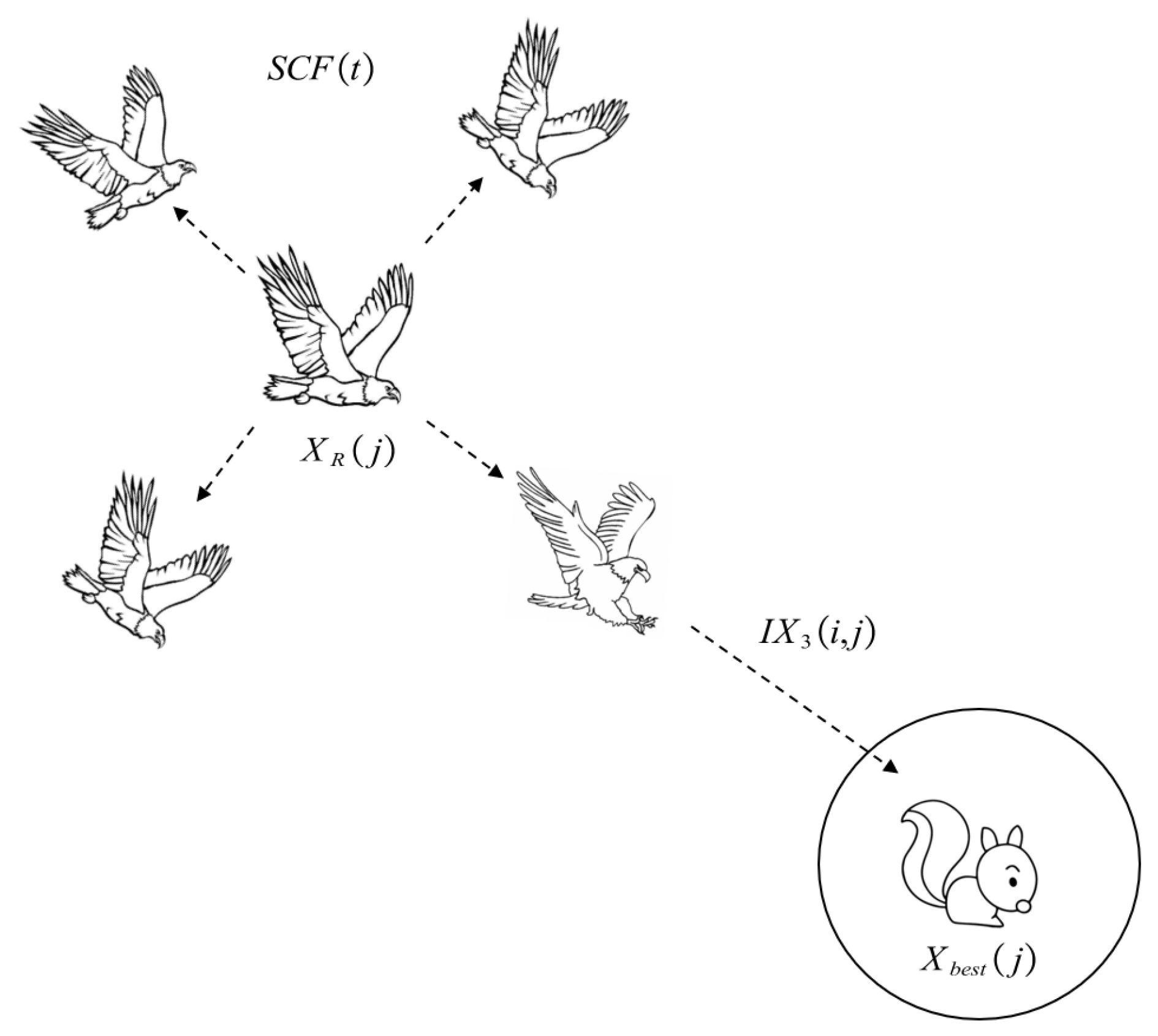
3.1.2. Improved Expanded Exploitation ($I{x}_3$): Search around Prey and Attack

In the third improved method, the Aquila searches thoroughly around the prey and then attacks it. Figure 2 shows this strategy, called Aquila search around prey and attack. This method aims to improve the exploitation capability, and is mathematically expressed by Equation (11):

$$I{X}_3\left(i,j\right)=L{B}_j+rand·\left(U{B}_j-L{B}_j\right)+R_7·\left(X_R\left(j\right)-X_{best}\left(j\right)\right)·SCF\left(t\right)·\left(1-\frac{t}{T}\right)$$

(11)

where $SCF\left(t\right)$ is the search control factor, $R_7$ and rand are random numbers between 0 and 1, $I{X}_3\left(i,j\right)$ is the solution of the next iteration of t, $X_{best}\left(j\right)$ represents the jth dimension of the best position in this current iteration, j is a random integer between 1 and the dimension length, $X_R\left(j\right)$ is the jth dimension of a random one selected from the Aquila population, and $L{B}_j$ and $U{B}_j$ represent the jth dimension of the the upper and lower bounds of the solution space, respectively.

3.2. Random Opposition-Based Learning (ROBL)

On the basis of opposition-based learning (OBL) [41], Long, W. [42] developed a powerful optimization tool called random opposition-based learning (ROBL). The main idea of ROBL is to consider the fitness of a solution and its corresponding random opposite solution at the same time in order to obtain a better candidate solution. ROBL has made a great contribution to improving exploitation ability, as defined by

$$X_L\left(t\right)=LB+UB-R_8\times X\left(t\right),$$

(12)

where $R_8$ is a random number between 0 and 1, $X_L\left(t\right)$ is the opposite solution, and $LB$ and $UB$ are the upper and lower bounds of the solution space, respectively.

3.3. Gaussian Mutation (GM)

Gaussian mutation (GM) is another commonly employed optimization tool, and performs well in the exploitation phase. Here, we use GM to prevent the IAO from falling into local optima; it is mathematically expressed by

$$X_G\left(t\right)=X\left(t\right)\times \left(1+Gaussian\left(\alpha \right)\right)$$

(13)

where $X\left(t\right)$ and $X_G\left(t\right)$ are the current and mutated positions, respectively, of a search agent and $Gaussian\left(\alpha \right)$ denotes a uniform random number that following a Gaussian distribution with a value of mean to 0 and standard deviation to 1, shown as

$$Gaussian\left(\alpha \right)=\frac{1}{\sqrt{2\pi {\sigma }^2}}·exp\left(-\frac{{\alpha }^2}{2{\sigma }^2}\right).$$

(14)

3.4. Computational Complexity of IAO

In this section, we discuss the computational complexity of the proposed IAO algorithm. In general, the computational complexity of the IAO typically includes three phases: initialization, fitness calculation, and updating of Aquila positions. The computational complexity of the initialization phase is O (N), where N is the population size of Aquila. Assume that T is the total number of iterations and O (T × N) is the computational complexity of the fitness calculation phase. Additionally, assume that Dim is the dimension of the problem; then, for updating positions of Aquila, the computational complexity is O (T × N × Dim + T × N × 2). Consequently, the total computational complexity of IAO is O (N × (T × (Dim + 2) + 1)).

3.5. Pseudo-Code of of IAO

In summary, IAO uses SCF to improve the second and third hunting methods of the original AO. Additionally, GM is applied to further enhance the exploitation capability, while ROBL is utilized to further improve the exploration phase. The target is to increase the solution diversity of the algorithm. The pseudocode and details of the IAO are shown in Algorithm 1 and Figure 3, respectively.

Algorithm 1 Improved Aquila Optimizer

1: Initialization phase: 2: Initialize the population X and the parameters of the IAO 3: while (The end condition is not met) do 4:      Calculate the fitness function values and $X_{best}\left(t\right)$: the best obtained solution 5:      for (i = 1, 2…, N) do 6:            Update the mean value of the current solution $X_M\left(t\right)$ and x, y, $G_1$, $G_2$, $Ly\left(D\right)$, etc. 7:            if $t\ll \left(\frac{2}{3}\right)T$ then 8:                   if $r⩽0.5$ then 9:                          Step 1: Expanded exploration ($X_1$) 10:                        Update the current solution using Equation (1) 11:                        $X_{new}\left(t+1\right)=X_1\left(t+1\right)$ 12:                 else 13:                        Step 2: Narrowed exploration ($I{X}_2$) 14:                        Update the current solution using Equation (10) 15:                        $X_{new}\left(t+1\right)=I{X}_2\left(t+1\right)$ 16:          else 17:                if $r⩽0.5$ then 18:                        Step 3: Expanded exploitation ($I{X}_3$) 19:                        Update the current solution using Equation (11) 20:                        $X_{new}\left(t+1\right)=I{X}_3\left(t+1\right)$ 21:                else 22:                        Step 4: Narrowed exploration ($X_4$) 23:                        Update the current solution using Equation (7) 24:                        $X_{new}\left(t+1\right)=X_4\left(t+1\right)$ 25:          if $Fitness\left(X_{new}\left(t+1\right)\right)<Fitness\left(X\left(t\right)\right)$ then 26:                $X\left(t\right)=X_{new}\left(t+1\right)$ 27:          Step 5: Random Opposition-Based Learning Updating ($X_L$) 28:          Update the current solution using Equation (12) 29:          if $Fitness\left(X_L\left(t\right)\right)<Fitness\left(X\left(t\right)\right)$ then 30:                $X\left(t\right)=X_L\left(t\right)$ 31:          Step 6: Gaussian-mutation Updating ($X_G$) 32:          Update the current solution using Equation (13) 33:          if $Fitness\left(X_G\left(t\right)\right)<Fitness\left(X\left(t\right)\right)$ then 34:                $X\left(t\right)=X_G\left(t\right)$ 35: return The best solution ($X_{best}$).

4. Experimental Results and Discussion

In this section, we desribe the 23 benchmark test functions, CEC2019 benchmark functions, and four real-world engineering design problems that were carried out to evaluate the performance of the IAO algorithm. To ensure the fairness of comparison, all algorithms were implemented for the same iterations and search agents, which were 500 and 30, respectively. All experiments were tested on the MATLAB 2019 platform using a PC with an Intel (R) Core (TM) i7-9750H CPU @ 2.60 GHz and 16 GB of RAM.

4.1. Results of Twenty-Three Benchmark Test Functions

In this section, we describe the 23 benchmark functions which were used to analyze the IAO’s ability in exploring the solution space and exploiting the global solutions. We used three types of benchmark functions: unimodal (F1-F7,

Table 2. Unimodal benchmark functions.

Fun	Dim	Range	Fmin
$f_1\left(x\right)={\sum }_{i=1}^n{x}_i^2$	10, 50, 100	[−100, 100]	0
$f_2\left(x\right)={\sum }_{i=0}^n\left|x_i\right|+{\prod }_{i=0}^n\left|x_i\right|$	10, 50, 100	[−10, 10]	0
$f_3\left(x\right)={\sum }_{i=1}^d{\left({\sum }_{j=1}^i{x}_j\right)}^2$	10, 50, 100	[−100, 100]	0
$f_4\left(x\right)={max}_i\left\{\left|x_i\right|,1⩽i\ll n\right\}$	10, 50, 100	[−100, 100]	0
$f_5\left(x\right)={\sum }_{i=1}^{n-1}\left[100{\left(x_i^2-x_{i+1}\right)}^2+{\left(1-x_i\right)}^2\right]$	10, 50, 100	[−30, 30]	0
$f_6\left(x\right)={\sum }_{i=1}^n{\left(\left[x_i+0.5\right]\right)}^2$	10, 50, 100	[−100, 100]	0
$f_7\left(x\right)={\sum }_{i=0}^{n}i{x}_i^4+random\left[0,\left.1\right)\right.$	10, 50, 100	[−128, 128]	0

), multimodal (F8-F13,

Table 3. Multimodal benchmark functions.

Fun	Dimensions	Range	Fmin
$f_8\left(x\right)={\sum }_{i=1}^n\left(-x_{i}sin\left(\sqrt{\left|x_i\right|}\right)\right)$	10, 50, 100	[−500, 500]	−418.9829n
$f_9\left(x\right)={\sum }_{i=1}^n\left[x_i^2-10cos\left(2\pi x_i\right)+10\right]$	10, 50, 100	[−5.12, 5.12]	0
$f_{10}\left(x\right)=-20exp\left(-0.2\sqrt{\frac{1}{n}{\sum }_{i=1}^n{x}_i^2}\right)-exp\left(\frac{1}{n}{\sum }_{i=1}^{n}cos\left(2\pi x_i\right)\right)+20+e$	10, 50, 100	[−32, 32]	0
$f_{11}\left(x\right)=1+\frac{1}{4000}{\sum }_{i=1}^n{x}_i^2-{\prod }_{i=1}^{n}cos\left(\frac{x_i}{\sqrt{i}}\right)$	10, 50, 100	[−600, 600]	0
$f_{12}\left(x\right)=\frac{\pi }{n}\left\{10sin\left(\pi y_1\right)\right\}+{\sum }_{i=1}^{n-1}{\left(y_i-1\right)}^2\left[1\right.+10{sin}^2\left(\pi y_{i+1}\right)+{\sum }_{i=1}^n\left.u\left(x_i,10,100,4\right)\right],$	10, 50, 100	[−50, 50]	0
$where{y}_i=1+\frac{x_i+1}{4},u\left(x_i,a,k,m\right)=\{\begin{array}{c}K{\left(x_i-a\right)}^m,if{x}_i>a\hfill \\ 0,-a⩽x_i⩾a\hfill \\ K{\left(-x_i-a\right)}^m,-a⩽x_i\hfill \end{array}$	10, 50, 100	[−50, 50]	0
$f_{13}\left(x\right)=0.1\left({sin}^2\left(3\pi x_1\right)\right.+{\sum }_{i=1}^n{\left(x_i-1\right)}^2\left[1+\right.{sin}^2\left.\left(3\pi x_1+1\right)\right]+{\left(x_n-1\right)}^{2}1+$	10, 50, 100	[−50, 50]	0
${sin}^2\left.\left(2\pi x_n\right)\right)+{\sum }_{i=1}^{n}u\left(x_i,5,100,4\right)$

), and fixed dimension multimodal functions (F14-F23,

Table 4. Fixed-dimension multimodal benchmark functions.

Fun	Dimensions	Range	Fmin
$f_{14}\left(x\right)={\left(\frac{1}{500}+{\sum }_{j=1}^{25}\frac{1}{j+{\sum }_{i=1}^2}\left(x_i-a_{ij}\right)\right)}^{-1}$	2	[−65, 65]	1
$f_{15}\left(x\right)={\sum }_{i=1}^{11}{\left[a_i-\frac{x_1\left({b_i}^2+b_i{x}_2\right)}{{b_i}^2+b_i{x}_3+x_4}\right]}^2$	4	[−5, 5]	0.0003
$f_{16}\left(x\right)=4{x_1}^2-2.1{x_1}^4+\frac{1}{3}{x_1}^6+x_1{x}_2-4{x_2}^2+4{x_2}^4$	2	[-5,5]	−1.0316
$f_{17}\left(x\right)={\left(x_2-\frac{5.1}{4{\pi }^2}{x_1}^2+\frac{5}{\pi }{x}_1-6\right)}^2+10\left(1-\frac{1}{8\pi }\right)cos{x}_1+10$	2	[−5, 5]	0.398
$f_{18}\left(x\right)=\left[\begin{array}{c}\begin{array}{c}1+{\left(x_1+x_2+1\right)}^2\left(\begin{array}{c}19-14x_1+3{x_1}^2-14x_2+6x_1{x}_2+\left.\left.3{x_2}^2\right)\right]\times \left[\begin{array}{c}30+{\left(2x_1-3x_2\right)}^2\end{array}\right.\end{array}\right.\end{array}\end{array}\right.$	2	[−2, 2]	3
$\times \left(\begin{array}{c}18-\end{array}\right.32x_i+12{x_1}^2+48x_2-36x_1{x}_2+\left.\left.27{x_2}^2\right)\right]$
$f_{19}\left(x\right)=-{\sum }_{i=1}^4{c}_{i}exp\left(-{\sum }_{i=1}^3{a}_{ij}{\left(x_j-p_{ij}\right)}^2\right)$	3	[−1, 2]	−3.86
$f_{20}\left(x\right)=-{\sum }_{i=1}^4{c}_{i}exp\left(-{\sum }_{i=1}^6{a}_{ij}{\left(x_j-p_{ij}\right)}^2\right)$	6	[0, 1]	−0.32
$f_{21}\left(x\right)=-{\sum }_{i=1}^5{\left[\left(X-a_i\right){\left(X-a_i\right)}^T+c_i\right]}^{-1}$	4	[0, 1]	−10.1532
$f_{22}\left(x\right)=-{\sum }_{i=1}^7{\left[\left(X-a_i\right){\left(X-a_i\right)}^T+c_i\right]}^{-1}$	4	[0, 1]	−10.4028
$f_{23}\left(x\right)=-{\sum }_{i=1}^{10}{\left[\left(X-a_i\right){\left(X-a_i\right)}^T+c_i\right]}^{-1}$	4	[0, 1]	−10.5363

). The results of unimodal and multimodal functions used to evaluate the exploitation ability and exploration tendency of IAO, respectively, in ten dimensions are shown in

Table 5. Results of the comparative methods on classical test functions (F1–F13); the dimension is fixed to 10.

Fun No.	Comparative Methods
Measure	IAO	AO	PSO	SCA	WOA	GWO	HBA	SMA	IHAOHHO	SNS
F1
Average	0.0000E+00	2.3224E-101	9.8827E-02	2.9790E-11	2.8930E-77	1.3870E-57	2.4460E-311	0.0000E+00	0.0000E+00	1.3155E-83
STD	0.0000E+00	1.2688E-100	1.7879E-01	1.6088E-10	1.3687E-76	4.3670E-57	0.0000E+00	0.0000E+00	0.0000E+00	4.0797E-83
F2
Average	0.0000E+00	8.2910E-54	2.1864E+00	2.8434E-09	1.0860E-52	3.4493E-33	2.5178E-165	3.7251E-165	0.0000E+00	1.9158E-43
STD	0.0000E+00	4.5332E-53	3.6831E+00	9.3310E-09	4.7689E-52	6.3477E-33	0.0000E+00	0.0000E+00	0.0000E+00	2.4764E-43
F3
Average	0.0000E+00	5.2357E-140	3.9463E+00	3.2085E-02	1.1925E+02	4.9961E-25	5.3850E-282	0.0000E+00	0.0000E+00	4.8278E-44
STD	0.0000E+00	2.3204E-139	8.2282E+00	1.1471E-01	2.0555E+02	2.2353E-24	0.0000E+00	0.0000E+00	0.0000E+00	1.1647E-43
F4
Average	0.0000E+00	1.7558E-53	1.4897E+00	1.1596E-03	4.7707E+00	3.1774E-18	4.1792E-151	7.5797E-169	0.0000E+00	7.0078E-39
STD	0.0000E+00	9.6168E-53	8.8025E-01	1.6691E-03	9.2981E+00	6.0564E-18	1.4627E-150	0.0000E+00	0.0000E+00	1.0665E-38
F5
Average	1.0280E-03	1.5008E-03	6.0458E+03	7.4225E+00	1.5318E+01	6.7390E+00	5.3561E+00	2.3140E+00	2.3893E-03	7.3809E+00
STD	4.0666E-03	1.7352E-03	2.2823E+04	4.4219E-01	4.5765E+01	8.2270E-01	4.9909E-01	2.9942E+00	3.4581E-03	2.7072E-01
F6
Average	3.1782E-07	1.7953E-05	6.7767E-02	4.4686E-01	3.2444E-03	8.4110E-03	9.8927E-09	4.2659E-05	2.5668E-06	6.2835E-06
STD	7.0485E-07	2.9948E-05	8.9846E-02	1.4309E-01	1.2638E-02	4.6050E-02	2.1026E-08	2.8976E-05	3.5834E-06	3.2982E-05
F7
Average	5.0112E-05	1.1823E-04	6.6253E-03	2.4664E-03	2.8474E-03	7.0323E-04	2.5156E-04	1.0642E-04	7.3335E-05	4.1179E-04
STD	3.7042E-05	8.6859E-05	5.1460E-03	2.0900E-03	2.8026E-03	4.3698E-04	3.4840E-04	1.0564E-04	8.0041E-05	2.6762E-04
F8
Average	−4.1898E+03	−2.7040E+03	−3.2063E+03	−2.1452E+03	−3.2492E+03	−2.6436E+03	−4.1125E+03	−4.1898E+03	−3.6604E+03	−4.1696E+03
STD	1.2752E-02	4.8263E+02	4.7583E+02	1.5916E+02	6.1201E+02	2.7699E+02	2.5316E+02	3.6702E-03	7.3765E+02	4.4751E+11
F9
Average	0.0000E+00	0.0000E+00	2.1168E+01	7.6524E-01	7.2367E-01	6.8404E-02	0.0000E+00	0.0000E+00	0.0000E+00	9.0618E-13
STD	0.0000E+00	0.0000E+00	1.1400E+01	2.6158E+00	3.9637E+00	3.7466E-01	0.0000E+00	0.0000E+00	0.0000E+00	3.9802E-12
F10
Average	8.8818E-16	8.8818E-16	2.1813E+00	4.8481E-07	4.4409E-15	7.7568E-15	8.8818E-16	8.8818E-16	8.8818E-16	8.8818E-16
STD	0.0000E+00	0.0000E+00	1.0373E+00	1.3528E-06	2.6389E-15	9.0135E-16	0.0000E+00	0.0000E+00	0.0000E+00	0.0000E+00
F11
Average	0.0000E+00	0.0000E+00	3.3710E-01	6.0756E-02	1.6105E-01	2.3521E-02	0.0000E+00	0.0000E+00	0.0000E+00	0.0000E+00
STD	0.0000E+00	0.0000E+00	1.9268E-01	9.2313E-02	1.9162E-01	2.4736E-02	0.0000E+00	0.0000E+00	0.0000E+00	0.0000E+00
F12
Average	3.0145E-07	5.8204E-06	4.2631E-01	1.2026E-01	6.7461E-02	3.3293E-03	6.2436E-04	3.9397E-06	1.3917E-06	6.3829E-09
STD	6.8979E-07	7.3875E-06	6.5028E-01	5.4482E-02	2.7273E-01	9.3149E-03	3.4190E-03	2.4780E-06	1.5261E-06	2.0490E-08
F13
Average	6.6465E-07	6.6356E-06	2.0431E-01	3.2588E-01	2.8072E-02	1.3021E-02	1.2726E-01	7.0433E-04	5.6927E-06	3.6630E-04
STD	8.8440E-07	8.7177E-06	2.0539E-01	8.8981E-02	3.6420E-02	3.3783E-02	1.1781E-01	5.4785E-04	6.5362E-06	2.0060E-03
(W|L|T)		(10|0|3)	(13|0|0)	(13|0|0)	(13|0|0)	(13|0|0)	(9|1|3)	(8|0|4)	(6|0|7)	(10|1|2)
Mean Rank	1.1538E+00	3.8462E+00	9.4615E+00	8.8462E+00	7.9231E+00	7.3077E+00	3.6154E+00	3.1538E+00	1.9231E+00	4.4615E+00
Final Rank	1	5	10	9	8	7	4	3	2	6

. In addition, these two tests were employed in 50 and 100 dimensions; the results are shown in

Table 6. Results of the comparative methods on classical test functions (F1–F13); the dimension is fixed to 50.

Fun No.	Comparative Methods
Measure	IAO	AO	PSO	SCA	WOA	GWO	HBA	SMA	IHAOHHO	SNS
F1
Average	0.0000E+00	1.2621E-98	1.3367E+03	9.8429E+02	4.9659E-73	9.3925E-20	2.6934E-268	3.1046E-303	0.0000E+00	2.2916E-69
STD	0.0000E+00	6.9126E-98	1.1120E+03	1.0716E+03	2.5168E-72	1.5742E-19	0.0000E+00	0.0000E+00	0.0000E+00	7.7994E-69
F2
Average	0.0000E+00	4.2713E-51	7.2861E+01	6.0782E-01	1.6283E-50	2.5761E-12	6.0605E-140	2.7294E-144	0.0000E+00	1.6968E-36
STD	0.0000E+00	2.3395E-50	2.8472E+01	5.8515E-01	7.0749E-50	2.3422E-12	3.2825E-139	1.4947E-143	0.0000E+00	1.7325E-36
F3
Average	0.0000E+00	6.2530E-99	1.9677E+04	4.8973E+04	2.0134E+05	6.9354E-01	2.7237E-230	1.3691E-255	0.0000E+00	3.1473E-19
STD	0.0000E+00	3.4230E-98	1.3525E+04	1.6184E+04	4.0176E+04	1.5062E+00	0.0000E+00	0.0000E+00	0.0000E+00	8.4013E-19
F4
Average	0.0000E+00	1.3486E-51	1.5811E+01	6.8791E+01	6.5347E+01	3.4044E-04	1.3771E-128	3.3920E-123	0.0000E+00	1.3513E-31
STD	0.0000E+00	6.1382E-51	4.2564E+00	8.6104E+00	2.9025E+01	2.5777E-04	4.9247E-128	1.3065E-122	0.0000E+00	1.8882E-31
F5
Average	6.2115E-02	8.7566E-03	1.6375E+05	8.0264E+06	4.8313E+01	4.7545E+01	4.7587E+01	1.5060E+01	6.7975E-02	4.8009E+01
STD	1.0885E-01	1.6222E-02	1.9275E+05	1.1260E+07	2.9790E-01	7.3129E-01	9.3529E-01	1.9174E+01	1.9964E-01	2.7176E-01
F6
Average	3.2391E-06	3.0053E-04	1.2981E+03	1.1480E+03	1.2141E+00	2.6191E+00	3.5202E+00	1.0294E-01	2.8225E-06	1.1414E+00
STD	3.7520E-06	4.6379E-04	4.6381E+02	9.0352E+02	4.7747E-01	5.3908E-01	8.0760E-01	1.1948E-01	4.0460E-06	4.0006E-01
F7
Average	4.5157E-05	1.0168E-04	5.9505E+00	3.7327E+00	2.6190E-03	3.0051E-03	3.7636E-04	1.9590E-04	9.5694E-05	5.5031E-04
STD	3.9634E-05	1.0872E-04	9.6585E+00	4.6774E+00	2.2822E-03	1.4242E-03	3.8930E-04	1.9448E-04	1.1017E-04	3.3177E-04
F8
Average	−2.0949E+04	−1.0296E+04	−1.0334E+04	−4.9128E+03	−1.8066E+04	−8.6995E+03	−2.0632E+04	−2.0945E+04	−2.0080E+04	−1.1343E+04
STD	1.0924E-01	6.4117E+03	1.1183E+03	3.4755E+02	2.8841E+03	1.6886E+03	4.8682E+02	3.9174E+00	2.5957E+03	7.7881E+02
F9
Average	0.0000E+00	0.0000E+00	3.2003E+02	1.0439E+02	0.0000E+00	4.5236E+00	0.0000E+00	0.0000E+00	0.0000E+00	0.0000E+00
STD	0.0000E+00	0.0000E+00	5.1219E+01	4.8147E+01	0.0000E+00	4.4977E+00	0.0000E+00	0.0000E+00	0.0000E+00	0.0000E+00
F10
Average	8.8818E-16	8.8818E-16	1.0035E+01	1.6811E+01	3.4935E-15	4.6984E-11	8.8818E-16	8.8818E-16	8.8818E-16	4.4409E-15
STD	0.0000E+00	0.0000E+00	4.7572E+00	6.7482E+00	2.6279E-15	1.8211E-11	0.0000E+00	0.0000E+00	0.0000E+00	0.0000E+00
F11
Average	0.0000E+00	0.0000E+00	1.2668E+01	9.2736E+00	0.0000E+00	2.6772E-03	0.0000E+00	0.0000E+00	0.0000E+00	0.0000E+00
STD	0.0000E+00	0.0000E+00	6.7658E+00	1.1111E+01	0.0000E+00	6.2169E-03	0.0000E+00	0.0000E+00	0.0000E+00	0.0000E+00
F12
Average	3.5676E-07	1.3093E-06	1.0947E+01	1.6926E+07	3.0187E-02	1.4397E-01	1.1742E-01	1.2283E-02	6.6027E-07	4.5960E-03
STD	5.9063E-07	2.1103E-06	6.0591E+00	2.1964E+07	2.5737E-02	7.7867E-02	7.7275E-02	1.7179E-02	8.6266E-07	3.7155E-03
F13
Average	3.1679E-06	2.5696E-05	7.5024E+02	2.9400E+07	1.1223E+00	2.0360E+00	4.1355E+00	2.4300E-02	1.5121E-05	3.3356E-01
STD	4.5408E-06	4.4035E-05	2.1952E+03	3.7851E+07	4.3282E-01	3.2325E-01	4.4922E-01	2.5096E-02	2.6993E-05	1.8665E-01
(W|L|T)		(9|1|3)	(13|0|0)	(13|0|0)	(11|0|2)	(13|0|0)	(10|0|3)	(10|0|3)	(6|0|7)	(10|0|3)
Mean Rank	1.0769E+00	3.3846E+00	9.1538E+00	9.4615E+00	6.0000E+00	7.5385E+00	4.2308E+00	3.0000E+00	1.6923E+00	4.7692E+00
Final Rank	1	4	9	10	7	8	5	3	2	6

and

Table 7. Results of the comparative methods on classical test functions (F1–F13); the dimension is fixed to 100.

Fun No.	Comparative Methods
Measure	IAO	AO	PSO	SCA	WOA	GWO	HBA	SMA	IHAOHHO	SNS
F1
Average	0.0000E+00	5.1159E-99	5.7117E+03	1.1443E+04	3.5827E-69	1.9290E-12	3.2518E-200	6.2811E-221	0.0000E+00	1.1048E-67
STD	0.0000E+00	2.8021E-98	3.6373E+03	8.2302E+03	1.9617E-68	1.2824E-12	0.0000E+00	0.0000E+00	0.0000E+00	4.1967E-67
F2
Average	0.0000E+00	3.9051E-52	1.5064E+02	7.2002E+00	2.2753E-50	4.2169E-08	1.3788E-111	1.2113E-141	0.0000E+00	3.2427E-35
STD	0.0000E+00	2.1383E-51	3.1696E+01	6.2087E+00	8.7244E-50	1.5009E-08	7.5522E-111	6.6348E-141	0.0000E+00	3.7736E-35
F3
Average	0.0000E+00	6.8311E-101	9.5308E+04	2.4323E+05	1.0637E+06	4.0890E+02	1.0078E-183	2.4850E-253	0.0000E+00	6.6454E-12
STD	0.0000E+00	2.5438E-100	6.2759E+04	6.0263E+04	2.4881E+05	3.7435E+02	0.0000E+00	0.0000E+00	0.0000E+00	3.6253E-11
F4
Average	0.0000E+00	2.0674E-54	2.1773E+01	8.8956E+01	7.2568E+01	1.0282E+00	9.8822E-98	7.2459E-140	0.0000E+00	1.9484E-30
STD	0.0000E+00	1.1324E-53	4.6161E+00	2.9508E+00	2.9428E+01	1.1412E+00	5.4126E-97	3.9688E-139	0.0000E+00	2.1891E-30
F5
Average	3.3067E-01	1.0799E-02	1.0524E+06	1.0779E+08	9.8209E+01	9.7923E+01	9.8033E+01	3.5374E+01	7.5137E+01	9.8128E+01
STD	4.1431E-01	2.0391E-02	1.0923E+06	6.9068E+07	2.1229E-01	6.6181E-01	6.8642E-01	4.0718E+01	4.2148E+01	2.5631E-01
F6
Average	1.7505E-05	1.4580E-03	4.4654E+03	1.3780E+04	4.3181E+00	1.0034E+01	1.3475E+01	1.6686E+00	7.8806E-05	7.7487E+00
STD	2.8122E-05	4.2895E-03	1.8531E+03	7.7723E+03	1.0995E+00	1.2448E+00	1.6622E+00	1.7329E+00	1.4201E-04	8.0349E-01
F7
Average	3.8993E-05	1.0242E-04	5.4957E+01	1.3007E+02	4.4602E-03	7.1806E-03	4.3691E-04	2.7884E-04	8.1182E-05	4.7715E-04
STD	3.3278E-05	7.1470E-05	1.2389E+02	5.2281E+01	5.5305E-03	4.0150E-03	8.6479E-04	2.2574E-04	5.9169E-05	2.8944E-04
F8
Average	−4.1898E+04	−1.1220E+04	−1.5662E+04	−6.9689E+03	−3.3889E+04	−1.5512E+04	−4.0452E+04	−4.1891E+04	−4.1647E+04	−1.8296E+04
STD	3.7073E-01	6.2868E+03	2.2964E+03	4.6480E+02	5.8967E+03	3.3937E+03	2.9790E+03	1.0217E+01	1.2765E+03	2.6919E+03
F9
Average	0.0000E+00	0.0000E+00	8.3584E+02	2.3748E+02	0.0000E+00	9.2482E+00	0.0000E+00	0.0000E+00	0.0000E+00	0.0000E+00
STD	0.0000E+00	0.0000E+00	4.4226E+01	1.2370E+02	0.0000E+00	8.1907E+00	0.0000E+00	0.0000E+00	0.0000E+00	0.0000E+00
F10
Average	8.8818E-16	8.8818E-16	1.0763E+01	2.0216E+01	3.8488E-15	1.2753E-07	8.8818E-16	8.8818E-16	8.8818E-16	4.4409E-15
STD	0.0000E+00	0.0000E+00	2.5471E+00	2.0674E+00	1.8853E-15	4.8362E-08	0.0000E+00	0.0000E+00	0.0000E+00	0.0000E+00
F11
Average	0.0000E+00	0.0000E+00	4.5743E+01	9.5013E+01	0.0000E+00	3.4526E-03	0.0000E+00	0.0000E+00	0.0000E+00	0.0000E+00
STD	0.0000E+00	0.0000E+00	1.5048E+01	6.1397E+01	0.0000E+00	9.1468E-03	0.0000E+00	0.0000E+00	0.0000E+00	0.0000E+00
F12
Average	1.1362E-07	1.7522E-06	1.7321E+02	3.6238E+08	4.9595E-02	3.0686E-01	3.5908E-01	1.4775E-02	4.3243E-07	4.7429E-02
STD	1.3745E-07	2.7432E-06	8.2035E+02	1.5973E+08	1.9496E-02	7.6135E-02	1.0260E-01	3.7190E-02	6.6715E-07	1.2802E-02
F13
Average	2.8163E-06	3.8493E-05	1.2104E+05	5.7687E+08	2.7539E+00	6.8028E+00	9.3862E+00	1.0836E-01	1.1256E-05	5.1031E+00
STD	3.2627E-06	4.6305E-05	2.3444E+05	2.6301E+08	8.5936E-01	4.9165E-01	4.6368E-01	2.0204E-01	2.0715E-05	9.5963E-01
(W|L|T)		(9|1|3)	(13|0|0)	(13|0|0)	(13|0|0)	(11|0|2)	(13|0|0)	(10|0|3)	(10|0|3)	(11|0|2)
Mean Rank	1.0769E+00	3.4615E+00	8.8462E+00	9.7692E+00	5.7692E+00	7.6154E+00	4.4615E+00	2.7692E+00	1.6923E+00	5.4615E+00
Final Rank	1	4	9	10	7	8	5	3	2	6

. Finally, the results with fixed dimension multimodal functions are shown in

Table 8. Results of the comparative methods on classical test functions (F14–F23).

Fun No.	Comparative Methods
Measure	IAO	AO	PSO	SCA	WOA	GWO	HBA	SMA	IHAOHHO	SNS
F14
Average	9.9800E-01	3.3268E+00	3.6091E+00	1.8685E+00	3.0570E+00	4.7152E+00	1.8474E+00	9.9800E-01	3.9338E+00	9.9800E-01
STD	1.9485E-07	5.2481E+00	3.9511E+00	1.5933E+00	3.4565E+00	4.4316E+00	2.4975E+00	4.2766E-13	4.1802E+00	3.1721E-17
F15
Average	3.4953E-04	5.2404E-04	1.0700E-02	1.0491E-03	6.0726E-04	4.4088E-03	3.1558E-03	5.2164E-04	3.7513E-04	3.6095E-04
STD	1.7826E-04	9.7738E-04	9.4417E-03	3.8370E-04	3.1958E-04	8.0603E-03	6.5715E-03	2.2777E-04	3.4012E-04	1.5460E-04
F16
Average	−1.0316E+00	−1.0316E+00	−1.0316E+00	−1.0316E+00	−1.0316E+00	−1.0316E+00	−1.0316E+00	−1.0316E+00	−1.0316E+00	−1.0316E+00
STD	2.4221E-06	1.6986E-03	2.9925E-16	6.9673E-05	3.1374E-09	3.2901E-08	9.1327E-08	1.6735E-09	7.0317E-10	2.4977E-16
F17
Average	3.9789E-01	3.9813E-01	3.9789E-01	3.9996E-01	3.9790E-01	3.9792E-01	3.9789E-01	3.9789E-01	3.9789E-01	3.9789E-01
STD	2.0640E-05	2.6541E-04	0.0000E+00	2.2873E-03	1.7337E-05	2.4586E-04	7.0378E-08	4.7990E-08	3.4610E-07	3.3645E-16
F18
Average	3.0000E+00	3.0308E+00	3.0000E+00	3.0001E+00	3.5402E+00	3.0000E+00	3.0000E+00	5.7000E+00	6.6000E+00	3.0000E+00
STD	2.6593E-04	2.0550E-05	1.8626E-15	1.8739E-04	3.8193E+00	5.6334E-05	1.7120E-15	1.1757E-10	8.2385E+00	1.3292E-15
F19
Average	−3.8626E+00	−3.8569E+00	−3.8615E+00	−3.8538E+00	−3.8571E+00	−3.8610E+00	−3.8628E+00	−3.8628E+00	−3.8627E+00	−3.8628E+00
STD	1.7812E-04	3.6747E-03	2.9875E-03	2.3179E-03	1.1745E-02	2.7863E-03	1.3914E-07	1.5881E-07	1.4671E-04	2.6684E-15
F20
Average	−3.2762E+00	−3.2488E+00	−3.1063E+00	−2.8254E+00	−3.1939E+00	−3.2652E+00	−3.2721E+00	−3.2425E+00	−3.2809E+00	−3.2911E+00
STD	5.9227E-02	1.0202E-01	2.6843E-01	4.2368E-01	1.7954E-01	7.6236E-02	5.9276E-02	5.7189E-02	5.8947E-02	5.2680E-02
F21
Average	−1.0153E+01	−1.0140E+01	−9.4095E+00	−2.4271E+00	−8.3139E+00	−9.3203E+00	−9.3280E+00	−1.0153E+01	−1.0153E+01	−1.0003E+01
STD	3.2810E-04	1.4970E-02	2.1134E+00	1.9289E+00	2.6107E+00	2.1197E+00	2.2797E+00	3.0386E-04	4.0101E-04	1.0639E+00
F22
Average	−1.0403E+01	−1.0402E+01	−8.7103E+00	−3.5346E+00	−7.4750E+00	−1.0084E+01	−9.1451E+00	−1.0403E+01	−1.0403E+01	−1.0297E+01
STD	4.9822E-04	1.8102E-03	3.0947E+00	1.9151E+00	3.0141E+00	1.2683E+00	2.9284E+00	2.3691E-04	1.9187E-04	7.5169E-01
F23
Average	−1.0536E+01	−1.0521E+01	−9.2431E+00	−3.7748E+00	−6.8094E+00	−1.0372E+01	−8.4938E+00	−1.0536E+01	−1.0536E+01	−1.0428E+01
STD	2.9928E-04	3.3891E-02	2.8229E+00	1.5647E+00	3.3590E+00	1.1473E+00	3.7874E+00	2.7799E-04	2.6806E-04	7.6480E-01
(W|L|T)		(9|0|1)	(6|1|3)	(9|0|1)	(8|1|1)	(6|2|2)	(7|0|3)	(4|0|6)	(4|1|5)	(5|1|4)
Mean Rank	1.600E+00	5.6000E+00	5.5000E+00	7.9000E+00	6.6000E+00	4.8000E+00	4.8000E+00	3.4000E+00	3.5000E+00	3.1000E+00
Final Rank	1	8	7	10	9	5	5	3	4	2

, indicating the exploration ability in the lower dimensions of the IAO. The results are compared with nine well-known algorithms: AO, PSO, SCA, WOA, GWO, HBA, SMA, IHAOHHO, and SNS. The main control parameters of the compared algorithms are shown in

Table 9. Parameters for the compared algorithms.

Algorithm	Parameters
AO	$U=0.00565;R_3=10;\omega =0.005;\alpha =0.1;\delta =0.1$
IHAOHHO	$U=0.00565;r_3=10;\omega =0.005;E=[2,0]$
PSO	$c_1=2;c_2=2;v_{max}=6$
SCA	–
WOA	$a=[2,0];b=2$
GWO	$a=[2,0]$
HBA	$C=2;\beta =6$
SMA	$z=0.03$
SNS	–

. All algorithms were evaluated using the mean and standard deviations (STD) from 30 independent runs and Friedman’s mean rank tests. Three lines of tables have been reported in order to display statistical analysis for the test functions, demonstrating the superiority of the IAO. The first line illustrates three symbols, (W|L|T), that denote the number of the functions in which the performance of the IAO was either the best (win), inferior (loss), or indistinguishable (tie) with respect to the compared algorithm. The second line shows the Friedman mean rank values., while the third line refers to the final rank values of the algorithms.

4.1.1. Qualitative Analysis for Convergence of IAO

In this section, we present the results of a series of experiments made to qualitatively analyze the convergence of the IAO. Figure 4 shows the parameter space of the function, search history of the Aquila positions, trajectory, average fitness, and convergence curve from the first to fifth columns, respectively. The search history reflects the way in which IAO explores and exploits the search space. The search history discusses how the Aquila explores and exploits the solution space, indicating the hunting behavior between the eagle and prey. From the last two columns, it can be seen that the values of average fitness and convergence curve are large at first, then gradually decrease as iteration progresses. From the fourth column, presenting the trajectory of the solution, it can be observed that the solution has a large value at the beginning of the iterations and gradually tends towards stability as iteration progresses. The comparison indicates that the IAO has strong exploitation and exploration abilities in the iterative process.

In addition, Figure 5 shows the convergence curve for the IAO and the other compared algorithms on the 23 benchmark functions. For unimodal functions (F1–F7), the convergence rate of the IAO is faster than the other algorithms, and its final convergence accuracy is better as well. This result confirms that the exploitation capacity of IAO is strong and has reliable performance. For the convergence curves of the multimodal functions, the IAO shows very good search performance. It can be seen that the IAO achieves a high balance between the exploration and exploitation phases. For F8–F15, F17, F21, F22, and F23, the IAO approaches positions around the optimal solutions at a very fast speed, and the positions have are exploited efficiently to catch the high precision final solutions. For F16, F18, F19, and F20, the IAO gradually approaches the optimal solutions and updates the Aquila positions in the iterations to confirm the final solution. In addition, three features can be obtained from Figure 5. The first is the fast convergence speed, which can be seen from F1–F4 and F9–F11. Second, from F5–F7, F12, F13, and F15, we can conclude that IAO has the best global optimal approximation compared with its peers. Finally, in examining the strong local optimum escape capability, the behavior of the IAO indicates its ability to escape the local optimum after multiple stagnations in F5–F7, F12, F13, and F20.

4.1.2. Exploitation Capability of IAO

Because the set of unimodal functions (F1-F7) has only one global optimum, it was employed to test the IAO’s exploitation capability, as shown in Table 5. From F1 to F4, the IAO can find the optimal solution. For F5 and F7, the IAO achieves the smallest average and STD values. For F6, the IAO shows the second smallest Average and STD, while HBA has the best. Therefore, as compared with other algorithms the IAO has the best stability and accuracy. It can be concluded that the exploitation capability of the IAO is excellent.

4.1.3. Exploration Capability of IAO

As multimodal functions have several local optima, they were employed to evaluate the IAO’s exploitation capability. The multimodal experiments were divided into two categories, multidimensional (F8–F13) and fixed-dimensional (F14–F23), to test the exploration ability of the IAO in multiple dimensions and low dimensions, respectively. From Table 5, it can be seen that the IAO attains the smallest Average and STD values, excluding F12. For F12, SNS performs best, while IAO achieves the second best position. As for the fixed-dimensional experiments, which are shown in Table 8, IAO achieves the best performance in more than half of the sets. These comparative trials show that IAO’s exploration capability is superior to its competitors.

4.1.4. Stability of IAO

To verify the stability and quality of IAO in dealing with high-dimensional problems, two more experiments were designed with dimensions of 50 and 100. All algorithms (IAO, AO, PSO, SCA, WOA, GWO, HBA, SMA, IHAOHHO, and SNS) were run independently 30 times with 30 search agents and 500 iterations. The results are shown in Table 6 and Table 7. It can be seen that the IAO obtains the best results in 50 and 100 dimensions except for the second performance in F5. For F5, AO obtains the minimum average and STD in both 50 and 100 dimensions. Therefore, we can conclude that the stability and quality of IAO confer a particularly good effect in dealing with high-dimensional problems.

4.1.5. Time Consuming Test of IAO

In this section, the running time of the algorithm is tested to evaluate its efficiency. Each algorithm was run in ten dimensions with variable dimension function (F1–F23) and the time was recorded. From

Table 10. Computation time of algorithms on benchmark functions.

Fun	Comparative Methods
	IAO	AO	PSO	SCA	WOA	GWO	HBA	SMA	IHAOHHO	SNS
F1	2.30E-01	1.11E-01	3.38E-02	5.18E-02	5.42E-02	6.23E-02	2.23E-01	4.09E-01	2.18E-01	1.93E-01
F2	2.22E-01	1.14E-01	3.56E-02	5.44E-02	4.87E-02	6.58E-02	2.01E-01	3.69E-01	2.17E-01	1.66E-01
F3	4.44E-01	2.25E-01	8.61E-02	9.06E-02	8.19E-02	9.94E-02	4.70E-01	4.49E-01	4.22E-01	1.92E-01
F4	2.09E-01	1.16E-01	3.47E-02	5.27E-02	6.77E-02	5.94E-02	1.85E-01	4.42E-01	2.10E-01	1.69E-01
F5	2.76E-01	1.42E-01	5.12E-02	6.90E-02	7.45E-02	7.68E-02	2.17E-01	4.17E-01	3.29E-01	1.80E-01
F6	2.04E-01	1.10E-01	3.50E-02	5.65E-02	4.53E-02	5.98E-02	2.21E-01	4.49E-01	2.21E-01	1.52E-01
F7	3.82E-01	1.64E-01	5.97E-02	7.48E-02	6.90E-02	8.45E-02	1.59E-01	4.27E-01	2.96E-01	1.74E-01
F8	2.52E-01	1.32E-01	4.73E-02	6.61E-02	6.04E-02	7.61E-02	1.16E-01	3.91E-01	2.77E-01	1.73E-01
F9	1.99E-01	1.13E-01	3.78E-02	5.59E-02	4.78E-02	6.65E-02	2.23E-01	3.85E-01	2.28E-01	1.71E-01
F10	2.43E-01	1.32E-01	3.98E-02	6.13E-02	5.19E-02	6.66E-02	2.55E-01	3.76E-01	2.29E-01	1.61E-01
F11	2.53E-01	1.37E-01	5.20E-02	7.12E-02	6.35E-02	7.87E-02	2.02E-01	3.96E-01	2.79E-01	1.71E-01
F12	8.22E-01	3.02E-01	1.43E-01	1.52E-01	1.42E-01	1.55E-01	6.28E-01	4.78E-01	6.55E-01	2.63E-01
F13	7.99E-01	3.21E-01	1.54E-01	1.46E-01	1.44E-01	1.60E-01	6.37E-01	4.48E-01	6.69E-01	2.90E-01
F14	2.28E+00	7.02E-01	3.78E-01	3.56E-01	3.80E-01	3.92E-01	1.64E-01	5.45E-01	1.65E+00	4.80E-01
F15	2.12E-01	1.08E-01	3.59E-02	4.70E-02	4.31E-02	5.16E-02	2.16E-01	2.70E-01	2.21E-01	1.80E-01
F16	2.52E-01	1.06E-01	3.51E-02	4.21E-02	4.29E-02	4.32E-02	1.57E-01	2.40E-01	2.12E-01	1.51E-01
F17	1.89E-01	1.17E-01	3.60E-02	3.66E-02	3.87E-02	4.11E-02	2.06E-01	2.73E-01	1.93E-01	1.49E-01
F18	1.69E-01	9.46E-02	2.91E-02	5.19E-02	3.58E-02	4.37E-02	1.89E-01	2.38E-01	1.86E-01	1.46E-01
F19	2.24E-01	1.17E-01	4.27E-02	5.42E-02	4.97E-02	5.31E-02	2.41E-01	2.62E-01	2.39E-01	1.65E-01
F20	2.60E-01	1.22E-01	4.12E-02	6.44E-02	6.28E-02	6.07E-02	1.82E-01	3.45E-01	2.45E-01	1.69E-01
F21	2.86E-01	1.43E-01	5.27E-02	6.58E-02	6.29E-02	6.79E-02	2.94E-01	3.60E-01	2.90E-01	1.83E-01
F22	4.03E-01	1.51E-01	6.33E-02	7.31E-02	8.77E-02	7.89E-02	3.26E-01	3.77E-01	3.19E-01	1.90E-01
F23	4.62E-01	1.68E-01	7.04E-02	8.54E-02	9.06E-02	8.67E-02	3.87E-01	3.00E-01	4.06E-01	2.33E-01

, it can be seen that the time required by IAO is longer than the original AO, as the GM and ROBL steps increase the complexity of the algorithm and consume excess time. Nevertheless, the elapsed time of IAO on the majority of the benchmark functions is less than that of SMA and IHAOHHO. Considering the excellent performance of the IAO and the increasing requirements of real-world optimization problems, the time consumption of the IAO is acceptable.

4.2. Results of Cec2019 Test Functions

This section analyses the IAO with the CEC2019 test functions, the definitions of which are listed in

Table 11. CEC2019 benchmark functions.

No.	Functions	Fmin	D	Search Range
1	Storn’s Chebyshev Polynomial Fitting Problem	1	9	[−8192, 8192]
2	Inverse Hilbert Matrix Problem	1	16	[−16384, 16384]
3	Lennard-Jones Minimun Energy Cluster	1	18	[−4, 4]
4	Rastrigin’s Function	1	10	[−100, 100]
5	Griewangk’s Function	1	10	[−100, 100]
6	Weierstrass Function	1	10	[−100, 100]
7	Modified Schwefel’s Function	1	10	[−100, 100]
8	Expanded Schaffer’s F6 Function	1	10	[−100, 100]
9	Happy Cat Function	1	10	[−100, 100]
10	Ackley Function	1	10	[−100, 100]

. The IAO was implemented with 30 agents and 500 iterations for 30 independent runs. The IAO was compared with AO, AOA, IHAOHHHO, PSO, HBA, WOA, and SSA. As reported in

Table 12. Results of the comparative methods on CEC2019 test functions.

Fun No.	Comparative Methods
Measure	IAO	AO	AOA	IHAOHHO	PSO	HBA	WOA	SSA
F1
Average	1.0000E+00	1.0000E+00	1.0000E+00	1.0000E+00	9.1426E+02	1.0000E+00	1.9196E+03	1.0000E+00
STD	0.0000E+00	7.0142E-08	1.3783E-11	0.0000E+00	1.2574E+03	1.0142E-15	1.9316E+03	0.0000E+00
F2
Average	4.9902E+00	5.0000E+00	4.8151E+00	4.9958E+00	2.3817E+01	4.4369E+00	4.7245E+01	5.0000E+00
STD	2.2790E-02	0.0000E+00	2.2630E-01	3.4360E-02	1.1027E+01	2.0940E-01	2.2419E+01	1.7967E-06
F3
Average	3.7124E+00	6.9735E+00	5.1734E+00	4.6995E+00	1.2112E+01	8.0559E+00	6.8170E+00	1.1024E+01
STD	1.1250E+00	1.8316E+00	1.5342E+00	2.7237E+00	8.5501E-01	2.7655E+00	2.7975E+00	2.4208E+00
F4
Average	3.7228E+01	3.8164E+01	5.8394E+01	6.5305E+01	5.9952E+01	5.5902E+01	5.9898E+01	8.3837E+01
STD	9.2662E+00	1.1124E+01	1.0801E+01	1.9889E+01	1.9166E+01	2.2363E+01	2.0615E+01	2.1308E+01
F5
Average	2.7378E+00	2.1021E+00	8.4194E+01	1.9913E+01	1.1439E+01	3.0982E+00	2.6868E+00	6.7515E+01
STD	3.2698E-01	1.9713E-01	3.1443E+01	1.4142E+01	9.1522E+00	5.7361E+00	8.2301E-01	3.7276E+01
F6
Average	6.2261E+00	5.4917E+00	1.0712E+01	1.0866E+01	8.9864E+00	8.1044E+00	9.1670E+00	1.1597E+01
STD	1.2281E+00	1.3587E+00	1.0793E+00	1.3478E+00	1.7271E+00	1.8066E+00	1.5338E+00	1.7529E+00
F7
Average	1.0325E+03	1.1475E+03	1.3246E+03	1.4688E+03	1.4088E+03	1.3097E+03	1.4174E+03	1.5311E+03
STD	2.8196E+02	2.9632E+02	2.1290E+02	3.9995E+02	2.5769E+02	4.0527E+02	2.7771E+02	3.5557E+02
F8
Average	4.3272E+00	4.4131E+00	4.7220E+00	4.8513E+00	4.6475E+00	4.7121E+00	4.8320E+00	4.9479E+00
STD	2.7159E-01	2.9467E-01	3.3237E-01	2.5891E-01	3.4308E-01	3.4192E-01	2.7793E-01	2.7781E-01
F9
Average	1.4783E+00	1.4901E+00	3.1939E+00	1.5746E+00	1.5590E+00	1.3615E+00	1.3896E+00	2.4654E+00
STD	1.4829E-01	1.3466E-01	6.0448E-01	4.3106E-01	4.1725E-01	1.7083E-01	1.9395E-01	8.8138E-01
F10
Average	2.0799E+01	2.0870E+01	2.1121E+01	2.1061E+01	2.1161E+01	2.1013E+01	2.1269E+01	2.1037E+01
STD	2.0220E+00	2.8398E+00	1.1769E-01	9.7112E-02	1.3506E-01	6.5911E-02	9.5167E-02	1.4888E-01
(W|L|T)		(7|2|1)	(8|1|1)	(9|0|1)	(10|0|0)	(7|2|1)	(8|2|0)	(9|0|1)
Mean Rank	1.7000E+00	3.0000E+00	4.7000E+00	5.2000E+00	5.7000E+00	2.9000E+00	5.4000E+00	6.3000E+00
Final Rank	1	3	4	5	7	2	6	8

, the comparison was performed through the average and STD values of the considered algorithms across the course of the functions. In addition, the Friedman mean rank values and final ranks are shown at the bottom of Table 12. The results confirm the proposed IAO’s superiority in dealing with these challenging test functions, as it performed the best in more than half of the functions.

4.3. Real-World Application

To further verify the performance of the algorithm, the IAO was tested in four well-known real-world engineering design problems: the speed reducer design problem, pressure vessel design problem, tension/compression spring design problem, and three-bar truss design problem, and the experimental results with the IAO were compared with classical algorithms proposed in previous studies.

4.3.1. Speed Reducer Design Problem

The optimization goal of this optimization problem is to minimize the weight of the speed reducer. This design problem includes seven optimization parameter variables and eleven constraints. Figure 6 shows the image expression of this design, and Equation (15) provides the mathematical expression. The IAO is compared with IHAOHHO, AO, AOA, PSO, SCA, GA, MDA, MFO, FA, HA, and PAO-DE. From

Table 13. Results of the compared algorithms for solving the speed reducer design problem.

Algorithm	Optimal Values for Variables							Optimum	Ranking
	${\mathit{x}}_1$	${\mathit{x}}_2$	${\mathit{x}}_3$	${\mathit{x}}_4$	${\mathit{x}}_5$	${\mathit{x}}_6$	${\mathit{x}}_7$	Weight
IAO	3.49711	0.7	17	7.3	7.7572	3.350613	5.286669	2995.4747	1
IHHOAO [40]	3.49924	0.7	17	7.3	7.8191	3.35006	5.28531	2996.0935	2
AO [37]	3.5021	0.7	17	7.3099	7.7476	3.3641	5.2994	3007.7328	6
AOA [34]	3.50384	0.7	17	7.3	7.72933	3.35649	5.2867	2997.9157	4
SCA [33]	3.508755	0.7	17	7.3	7.8	3.46102	5.289213	3030.563	10
GA [13]	3.510253	0.7	17	8.35	7.8	3.362201	5.287723	3067.561	11
MDA [43]	3.5	0.7	17	7.3	7.670396	3.542421	5.245814	3019.583365	8
MFO [44]	3.49745	0.7	17	7.82775	7.71245	3.35178	5.28635	2998.9408	5
FA [45]	3.507495	0.7001	17	7.71967	8.08085	3.35151	5.28705	3010.137492	7
HS [46]	3.520124	0.7	17	8.37	7.8	3.36697	5.288719	3029.002	9
PSO-DE [47]	3.5	0.7	17	7.3	7.8	3.35021	5.28668	2996.3481	3

, it can be seen hat the IAO is superior to all of the other algorithms, and ranks first.

Minimize

$$\begin{array}{c}\hfill f\left(\overrightarrow{x}\right)=0.7854x_1{x}_2^2\left(3.3333x_3^2+14.9334x_3-43.0943\right)\\ \hfill -1.508x_1\left(x_6^2+x_7^2\right)+7.4777\left(x_6^3+x_7^3\right)\end{array}$$

(15)

Subject to

$$\begin{array}{c}\hfill g_1\left(\overrightarrow{x}\right)=\frac{27}{x_1{x}_2^2{x}_3}-1\ll 0\\ \hfill g_2\left(\overrightarrow{x}\right)=\frac{397.5}{x_1{x}_2^2{x}_2^2}-1\ll 0\\ \hfill g_3\left(\overrightarrow{x}\right)=\frac{1.93x_4^3}{x_2{x}_3{x}_6^4}-1\ll 0\\ \hfill g_4\left(\overrightarrow{x}\right)=\frac{1.93x_5^3}{x_2{x}_3{x}_7^4}-1\ll 0\\ \hfill g_5\left(\overrightarrow{x}\right)=\frac{\sqrt{{\left(\frac{745x_4}{x_2{x}_3}\right)}^2+16.9\times {10}^6}}{110x_6^3}-1\ll 0\\ \hfill g_6\left(\overrightarrow{x}\right)=\frac{\sqrt{{\left(\frac{745x_4}{x_2{x}_3}\right)}^2+157.5\times {10}^6}}{85x_6^3}-1\ll 0\\ \hfill g_7\left(\overrightarrow{x}\right)=\frac{x_2{x}_3}{40}-1\ll 0\\ \hfill g_8\left(\overrightarrow{x}\right)=\frac{5x_2}{x_1}-1\ll 0\\ \hfill g_9\left(\overrightarrow{x}\right)=\frac{x_1}{12x_2}-1\ll 0\\ \hfill g_{10}\left(\overrightarrow{x}\right)=\frac{1.5x_6+1.9}{x_4}-1\ll 0\\ \hfill g_{11}\left(\overrightarrow{x}\right)=\frac{1.1x_7+1.9}{x_5}-1\ll 0\end{array}$$

(16)

where $2.6⩽x_1⩽3.6,0.7⩽x_2⩽0.8,17⩽x_3⩽28,7.3⩽x_4⩽8.3,7.8⩽x_5⩽8.3,2.9⩽x_6⩽3.9,5⩽x_7⩽5.5.$

4.3.2. Pressure Vessel Design Problem

The optimization goal of this design problem is to minimize the manufacturing cost of pressure vessels. As shown in Figure 7, this design problem includes four variables that need to be optimized: the thickness of the shell (Ts), the head (Th), the length of the cylindrical section (L), and the inner radius (R). Meanwhile, there are four constraints, as shown below. From

Table 14. Results of the compared algorithms for solving the pressure vessel design problem.

Algorithm	Optimal Values for Variables				Optimum	Ranking
	${\mathit{T}}_{\mathit{s}}$	${\mathit{T}}_{\mathit{h}}$	R	L	Weight
IAO	0.7788354	0.3871472	40.35416	199.5197	5892.7534	1
AO [37]	1.054	0.182806	59.6219	38.805	5949.2258	3
IHHOAO [40]	0.8363559	0.4127868	45.08462	142.9202	5932.3392	2
WOA [31]	0.8125	0.4375	42.0982699	176.638998	6059.741	9
SMA [27]	0.7931	0.3932	40.6711	196.2178	5994.1857	4
GWO [30]	0.8125	0.4345	42.0892	176.7587	6051.5639	6
AOA [34]	0.8303737	0.4162057	42.75127	169.3454	6048.7844	5
PSO-SCA [47]	0.8125	0.4375	42.098446	176.6366	6059.71433	8
MVO [11]	0.8125	0.4375	42.090738	176.73869	6060.8066	12
GA [13]	0.8125	0.4375	42.097398	176.65405	6059.94634	11
HPSO [48]	0.8125	0.4375	42.0984	176.6366	6059.7143	7
ES [49]	0.8125	0.4375	42.098087	176.640518	6059.7456	10

, it can be seen that the results with the IAO are the best compared to its competitors.

Consider $\overrightarrow{x}=\left[x_1{x}_2{x}_3{x}_4\right]=\left[T_s{T}_{h}RL\right]$

Minimize

$$f\left(\overrightarrow{x}\right)=0.6224x_1{x}_3{x}_4+1.7781x_2{x}_3^2+3.1661x_1^2{x}_4+19.84x_1^2{x}_3$$

(17)

Subject to

$$\begin{array}{c}\hfill g_1\left(\overrightarrow{x}\right)=-x_1+0.0193x_3\ll 0\\ \hfill g_2\left(\overrightarrow{x}\right)=-x_2+0.00954x_3\ll 0\\ \hfill g_3\left(\overrightarrow{x}\right)=-\pi x_3^2{x}_4-\frac{4}{3}\pi x_3^3+1296000\ll 0\\ \hfill g_4\left(\overrightarrow{x}\right)=x_4-240\ll 0\end{array}$$

(18)

where $0\ll x_1\ll 99,0\ll x_2\ll 99,10\ll x_3\ll 200,10\ll x_4\ll 200$

4.3.3. Tension/Compression Spring Design Problem

This design problem seeks to minimize the weight of the tension/compression spring by adjusting three design variables: the wire diameter (d), mean coil diameter (D), and the number of active coils (N), shown in Figure 8. Equation (19) provides the mathematical functions of this problem. The results can be obtained from

Table 15. Results of the compared algorithms for solving the tension/compression spring design problem.

Algorithm	Optimal Values for Variables			Optimum	Ranking
	d	D	N	Weight
IAO	0.051827941	0.364475012	10.7068472	0.012440375	3
AO [37]	0.0502439	0.35262	10.5425	0.011165	2
IHAOHHO [40]	0.055883	0.52784	4.7603	0.011144	1
WOA [31]	0.051207	0.345215	12.004032	0.0126763	7
HS [46]	0.051154	0.349871	12.076432	0.0126706	5
MVO [11]	0.05251	0.37602	10.33513	0.01279	9
PSO [50]	0.051728	0.357644	11.244543	0.0126747	6
ES [49]	0.051643	0.355360	11.397926	0.012698	8
CSCA [51]	0.051609	0.354714	11.410831	0.0126702	4

, where it can be seen that the IAO is competitive compared with AO, IHAOHHO, WOA, HS, MVO, PSO, ES, and CSCA.

Consider $\overrightarrow{x}=\left[x_1{x}_2{x}_3\right]=\left[dDN\right]$

Minimize

$$f\left(\overrightarrow{x}\right)=\left(x_3+x_2\right)x_2{x}_1^2$$

(19)

Subject to

$$\begin{array}{c}\hfill g_1\left(\overrightarrow{x}\right)=1-\frac{x_2^3{x}_3}{71785x_1^4}\ll 0\\ \hfill g_2\left(\overrightarrow{x}\right)=\frac{4x_2^2-x_1{x}_2}{12566\left(x_2{x}_1^3-x_1^4\right)}+\frac{1}{5108x_1^2}\ll 0\\ \hfill g_3\left(\overrightarrow{x}\right)=1-\frac{140.45x_1}{x_2^2{x}_3}\ll 0\\ \hfill g_4\left(\overrightarrow{x}\right)=\frac{x_1+x_2}{1.5}-1\ll 0\end{array}$$

(20)

where $0.05⩽x_1⩽2,0.25⩽x_2⩽1.30,2.00⩽x_3⩽15$.

4.3.4. Three-Bar Truss Design Problem

This design problem seeks to minimize the weight of the truss by adjusting the two parameters in Figure 9. Equation (21) provides the mathematical functions of the problem. The results are shown in

Table 16. Results of the compared algorithms for solving three-bar truss design problem.

Algorithm	Optimal Values for Variables		Optimum	Ranking
	${\mathit{x}}_1$	${\mathit{x}}_2$	Weight
IAO	0.7912217	0.4007014	263.8614364	1
AO [37]	0.7926	0.3966	263.8684	3
IHHOAO [40]	0.79002	0.40324	263.8622	2
AOA [34]	0.79369	0.39426	263.9154	9
SSA [32]	0.78866541	0.408275784	263.89584	4
MBA [52]	0.788565	0.4085597	263.89585	6
PSO-DE [47]	0.7886751	0.4082482	263.89584	5
CS [53]	0.78867	0.40902	263.9716	10
GOA [54]	0.788897556	0.40761957	263.8958815	7
MFO [44]	0.788244771	0.409466906	263.8959797	8

, from which it is obvious that the IAO can better obtain the minimum weight of a three-bar truss compared with AO, IHAOHHO, AOA, SSA, MBA, PSO-DE, CS, GOA, and MFO.

Minimize

$$f\left(\overrightarrow{x}\right)=\left(2\sqrt{2x_1}+x_2\right)\times l$$

(21)

Subject to

$$\begin{array}{c}\hfill g_1\left(\overrightarrow{x}\right)=\frac{\sqrt{2x_1}+x_2}{\sqrt{2x_1^2}+2x_1{x}_2}P-\sigma \ll 0\\ \hfill g_2\left(\overrightarrow{x}\right)=\frac{x_2}{\sqrt{2x_1^2}+2x_1{x}_2}P-\sigma \ll 0\\ \hfill g_3\left(\overrightarrow{x}\right)=\frac{1}{\sqrt{2x_2}+x_1}P-\sigma \ll 0\end{array}$$

(22)

where $0⩽x_1\ll 1,0⩽x_2\ll 1,l=100\mathrm{cm},P=2{\mathrm{KN}/\mathrm{cm}}^2,and\sigma =2{\mathrm{KN}/\mathrm{cm}}^2.$

5. Conclusions

This paper proposes an Improved Aquila Optimizer (IAO) algorithm. A search control factor (SCF) is proposed to improve the second and third search strategies of the original Aquila Optimizer (AO) algorithm. Then, GM and ROBL methods are integrated to further improve the exploration and exploitation ability of the original AO. To evaluate the performance of the IAO, we tested the algorithm with 23 benchmark functions and CEC2019 test functions. From the results, the performance of the IAO is superior to other advanced MH algorithms. Meanwhile, through experimental results on four real-world engineering design problems, it is validated that the IAO has high practicability in solving practical problems.

In future studies, we will consider various methods to balance the exploration and exploitation phases. Different mutation strategies can be taken into account to increase the solution diversity. In addition, the proposed algorithm could be applied to more fields, including deep learning, material scheduling problems, parameter estimation, wireless sensor networks, path planning, signal denoising, image segmentation, model optimization, and more.